


Gradients are needed not only for constructing values of a scalar at the cell faces, but also for computing secondary diffusion terms and velocity derivatives. For more information about the different gradients, see Evaluation of Gradients and Derivatives in the Theory Guide.
The three gradients that are available in Ansys Fluent are
Green-Gauss Cell Based
Green-Gauss Node Based
Least Squares Cell Based
The gradient options are selectable from the Gradient drop-down list, in the Solution Methods task page.
![]() Solution →
Solution → ![]() Methods
Methods
In addition, Ansys Fluent allows you to choose the discretization scheme for the convection terms of each governing equation. (Second-order accuracy is automatically used for the viscous terms.) By default, single-phase problems using either the pressure-based or density-based solver are solved using second-order upwind discretization for the convection terms of the flow equations and all scalar equations except those for turbulence quantities, which are solved using first-order upwind discretization. For multiphase flows, the flow equations use first-order upwind discretization by default. For a complete description of the discretization schemes available in Ansys Fluent, see Discretization in the Theory Guide.
In addition, when you use the pressure-based solver, you can specify the pressure interpolation scheme. For a description of the pressure interpolation schemes available in Ansys Fluent, see Pressure Interpolation Schemes in the Theory Guide.
For additional information, see the following sections:
When the flow is aligned with the mesh (for example, laminar flow in a rectangular duct modeled with a quadrilateral or hexahedral mesh) the first-order upwind discretization may be acceptable. When the flow is not aligned with the mesh (that is, when it crosses the mesh lines obliquely), however, first-order convective discretization increases the numerical discretization error (numerical diffusion). For triangular and tetrahedral meshes, since the flow is never aligned with the mesh, you will generally obtain more accurate results by using the second-order discretization. For quad/hex meshes, you will also obtain better results using the second-order discretization, especially for complex flows.
In summary, while the first-order discretization generally yields better convergence than the second-order scheme, it generally will yield less accurate results, especially on tri/tet meshes. See Convergence and Stability for information about controlling convergence.
For most cases, you will be able to use the second-order scheme from the start of the calculation. In some cases, however, you may need to start with the first-order scheme and then switch to the second-order scheme after a few iterations. For example, if you are running a high-Mach-number flow calculation that has an initial solution much different than the expected final solution, you will usually need to perform a few iterations with the first-order scheme and then turn on the second-order scheme and continue the calculation to convergence. Alternatively, full multigrid initialization is also available for some flow cases that allow you to proceed with the second-order scheme from the start.
For a simple flow that is aligned with the mesh (for example, laminar flow in a rectangular duct modeled with a quadrilateral or hexahedral mesh), the numerical diffusion will be naturally low, so you can generally use the first-order scheme instead of the second-order scheme without any significant loss of accuracy.
Finally, if you run into convergence difficulties with the second-order scheme, you should try the first-order scheme instead.
While the higher-order scheme may result in greater accuracy, it can also result in convergence difficulties and instabilities at certain flow conditions. On the other hand, using a first-order scheme may not provide the desired accuracy. One approach to achieving improved accuracy while maintaining good stability is to use a discretization blending factor. This feature is available for both density-based and pressure-based solvers and can be invoked using the following text command:
solve → set → numerics
Enter a value between 0 and 1 when asked for the blending factor:
1st-order to higher-order blending factor [min=0.0 - max=1.0]
A blending factor of 0 reduces the gradient reconstruction to a first-order discretization scheme,
whereas 1 will recover high-order discretization. A blending factor of less than
1 (typically 0.75 or 0.5) will make the convective fluxes more diffusive, which in some flow conditions
can stabilize a solution that is otherwise unstable when the full higher-order discretization scheme is employed.
Important: Note that in order to use this feature effectively, make sure that one of the allowed higher-order discretization schemes is selected for the desired variables in the Solution Methods task page.
The QUICK and third-order MUSCL discretization schemes may provide better accuracy than the second-order scheme for rotating or swirling flows. The QUICK scheme is applicable to quadrilateral or hexahedral meshes, while the MUSCL scheme is used on all types of meshes. In general, however, the second-order scheme is sufficient and the QUICK scheme will not provide significant improvements in accuracy.
Important: If QUICK is used for hybrid meshes, it will be used only for quadrilateral and hexahedral cells. Second-order upwind discretization will be applied to all other cells.
The bounded central differencing and (for the pressure-based solver) central differencing schemes are available when you are using the LES, DES, SAS, SBES, and SDES turbulence models, and the central differencing scheme should be used only when the mesh spacing is fine enough so that the magnitude of the local Peclet number is less than 1. The Peclet number is defined as [114], [115]:
 | (36–1) |
where  is the fluid density,
  is local cell velocity,
  is a length scale (for example, mesh size), and
  is the diffusion coefficient of the fluid.
If you select the bounded central differencing scheme, you have the option to specify the BCD Scheme Boundedness as a constant or expression. For more details, see Bounded Central Differencing Scheme in the Fluent Theory Guide.
A modified HRIC scheme (see Modified HRIC Scheme in the Theory Guide) is also available for VOF simulations using either the implicit or explicit formulation.
As discussed in Pressure Interpolation Schemes in the Theory Guide, a number of pressure interpolation schemes are available when the pressure-based solver is used in Ansys Fluent. For most single-phase cases, the second-order scheme is acceptable, but some types of models may benefit from one of the other schemes:
For flows with high swirl numbers, high-Rayleigh-number natural convection, high-speed rotating flows, and flows in strongly curved domains, the PRESTO! scheme is recommended.
For problems involving large body forces, the Body Force Weighted scheme is recommended.
For Eulerian multiphase models, the default scheme is PRESTO!. However, for multi-fluid VOF problems that use the non-iterative solver, the Second Order interpolation scheme can be more robust for cases with skewed meshes, and the Body Force Weighted interpolation scheme can be more robust for cases with large body forces and skewed meshes.
For VOF and Mixture multiphase models, either the PRESTO! (default) or Modified Body Force Weighted scheme should be used:
The PRESTO! scheme is more comprehensive than the other schemes.
The Modified Body Force Weighted scheme is a good alternative to both PRESTO! and Body Force Weighted for most problems. It exhibits less sensitivity to mesh and time-step sizes compared to the PRESTO! scheme.
The Modified Body Force Weighted scheme is recommended for:
the non-iterative solver (as it offers better robustness)
cases where large body forces are present
The scheme can be used for highly viscous and rotating flows where the Body Force Weighted scheme has severe limitations.
As discussed in Density Interpolation Schemes in the Theory Guide, four density interpolation schemes are available when the pressure-based solver is used to solve a single-phase compressible flow.
The second-order upwind scheme (the default) provides reasonable stability for the discretization of the pressure-correction equation, and gives good results for most classes of flows. The first-order upwind scheme will provide greater stability, but may tend to smooth shocks in compressible flows. If you are calculating a compressible flow with shocks you should use the second-order-upwind or QUICK scheme. Using the QUICK scheme for all variables, including density, is highly recommended for compressible flows with shocks when using quadrilateral, hexahedral, or hybrid meshes. The third-order MUSCL scheme is applicable to arbitrary meshes and has the potential to improve spatial accuracy for all types of meshes by reducing numerical diffusion.
Important: In the case of multiphase flows, the selected density scheme is applied to the compressible phase and arithmetic averaging is used for incompressible phases.
The purpose of the relaxation of high order terms is to improve the startup and the general solution behavior of flow simulations when higher order spatial discretizations are used (higher than first). It has also shown to prevent convergence stalling in some cases. Such high-order terms can be of significant importance in certain cases and lead to numerical instabilities. This is particularly true at aggressive solution settings. In such cases, high order relaxation is a useful strategy to minimize your interaction during the solution. This can be an effective alternative to starting the solution first order, then switching to second order spatial discretization at a later stage.
The High Order Term Relaxation option can be enabled from the Solution Methods task page, as shown in Figure 36.2: The Solution Methods Task Page for the HOTR Option.
![]() Solution →
Solution → ![]() Methods
Methods
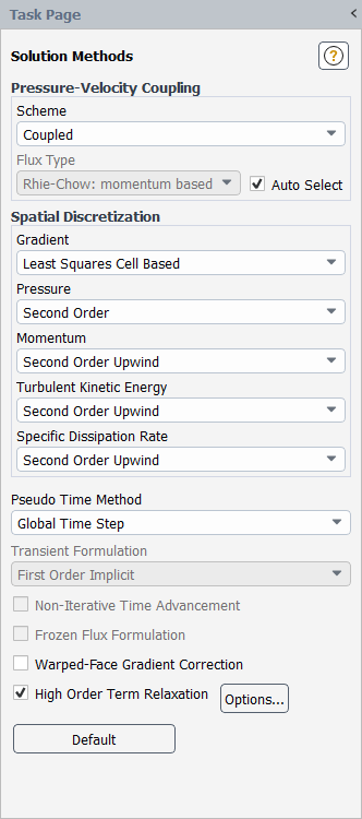
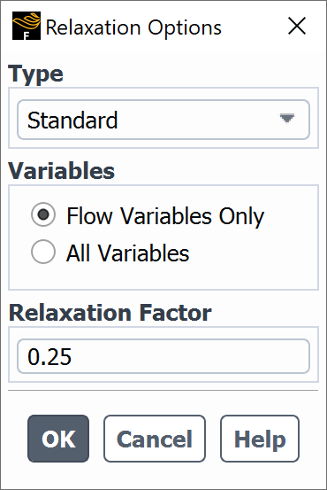
Further control of High Order Term Relaxation can be obtained after clicking and making the necessary selections and settings in the Relaxation Options dialog box (Figure 36.3: The Relaxation Options Dialog Box with the Pressure-Based Solver).
When using the pressure-based solver, you can select the Type of HOTR that you would like to apply:
Standard
HOTR is applied to both convection and diffusion terms. This is the default selection.
Convection Only
HOTR is applied to exclusively to the convection terms. This has the potential to deepen and accelerate convergence for some cases, such as steady-state turbomachinery simulations that use the default SST
 -
- turbulence model.
For both the pressure-based and the density-based solvers, you have the option of selecting All Variables to be under-relaxed instead of only the default flow variables (Flow Variables Only).
If you select Flow Variables Only, then the following variables will be under-relaxed:
Velocity components
Pressure
Energy
Density
Turbulence quantities (excluding Reynolds stresses)
Volume fraction
If you select All Variables, then relaxation is applied to each variable discretized with a higher order scheme.
The default values for the Relaxation Factor is 0.25 for steady-state cases and 0.75 for transient cases. The same factor is applied to all equations solved.
For theoretical information about high order term relaxation, see High Order Term Relaxation in the Theory Guide.
The following limitations exist when using the High Order Term Relaxation option:
The High Order Term Relaxation option is not available when the Non-Iterative Time Advancement option is enabled, since the simulation would not achieve the required level of high order spatial accuracy.
In general, high order term relaxation is available for transient flows. Nevertheless, it should be used with care. To achieve high order accuracy at convergence for each time step, you must increase the number of iterations per time step to ensure that the original convergence criteria have been met.
When the QUICK scheme is selected for specific transport equations, no under-relaxation is applied to this equation.
You can specify the discretization scheme and, for the pressure-based solver, the pressure interpolation scheme in the Solution Methods Task Page (Figure 36.4: The Solution Methods Task Page for a Pressure-Based Segregated Algorithm).
![]() Solution →
Solution → ![]() Methods
Methods
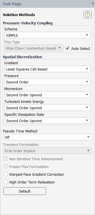
For each scalar equation listed under Spatial Discretization (Momentum, Energy, Turbulent Kinetic Energy, and so on, for the pressure-based solver or Turbulent Kinetic Energy, Turbulent Dissipation Rate, and so on, for the density-based solver) you can choose First Order Upwind, Second Order Upwind, QUICK, Third-Order MUSCL, or (for Momentum when you are using the LES, DES, SAS, SDES, or SBES turbulence model) Bounded Central Differencing (the default) or Central Differencing in the adjacent drop-down list. For the density-based solver, you can choose either First Order Upwind, Second Order Upwind, Third-Order MUSCL, or (when you are using the LES, DES, SAS, SDES, or SBES turbulence model) Bounded Central Differencing for the Flow equations (which include momentum and energy). Note that the task page shown in Figure 36.4: The Solution Methods Task Page for a Pressure-Based Segregated Algorithm is for the pressure-based solver.
If you are using the pressure-based solver, select the pressure interpolation scheme under Spatial Discretization, in the drop-down list next to Pressure. You can choose Standard, PRESTO!, Linear, Second Order, Body Force Weighted, or Modified Body Force Weighted.
Important: The low-order formulation of PRESTO! can be applied by limiting the high-order terms for the PRESTO! scheme. This is done using the following text command:
solve → set → numerics
When asked limit high-order terms for PRESTO! pressure scheme?, enter yes.
This modification can be used to stabilize the solution process when the pressure-based coupled algorithm is used and when the original PRESTO! scheme either fails to converge or produces unphysical oscillations (wiggles) in the pressure field.
If you are using the pressure-based solver and your flow is compressible (that is, you are using the ideal gas law for density), select the density interpolation scheme under Spatial Discretization, in the drop-down list next to Density. You can choose First Order Upwind, Second Order Upwind, QUICK or Third-Order MUSCL. (Note that Density will not appear for incompressible flows.)
If you enable the VOF model while using the pressure-based solver, the volume fraction interpolation schemes that are available are Geo-Reconstruct, CICSAM, Modified HRIC, Compressive, and QUICK.
If your case involves species transport, you can set the scheme for the individual species as First Order Upwind, Second Order Upwind, QUICK, or Third-Order MUSCL. However, if you want all your species to use the same discretization scheme, then rather than setting each one individually, simply enable the Set All Species Discretizations Together option. Notice that you will no longer see your list of individual species, instead a Species field will appear with the scheme of your choice.
If you change the settings for the Spatial Discretization, but you then want to return to Ansys Fluent’s default settings, you can click the button.
Important: If your mesh topology has step-wise prism mesh near the walls, do not use node-based gradients with MUSCL.