


Use Separating, Morphing, Adaptive and Remeshing Technology (SMART) to simulate both static and fatigue crack-growth in engineering structures.
SMART updates the mesh from crack-geometry changes due to crack-growth automatically at each solution step. Mesh updates occur around the crack-front region only and are integrated into the Mechanical APDL solver without exiting and reentering the solver, resulting in a computationally efficient solution of the crack-growth problem.
Crack-growth mechanics include various fracture criteria for static crack-growth and fatigue crack-growth.
SMART supports distributed-memory parallel processing.
Primary analysis characteristics:
Linear elastic isotropic materials only.
Uses SOLID187 only.
Ignores large-deflection and finite-rotation effects, crack-tip plasticity effects, and compression effects.
Fracture criteria for static crack-growth include critical stress-intensity factor and J-integral.
Fatigue crack-growth is based on Paris' Law, Walker equation, Forman equation, tabular fatigue law (
 vs.
vs.  ), or NASGRO equation v. 3 or
v. 4.
), or NASGRO equation v. 3 or
v. 4.A fatigue crack-closure effect can be included via the Elber closure function, Schijve closure function, Newman closure function, or polynomial closure function.
Loading considerations:
For static crack-growth analysis, enable automatic time-stepping (AUTOTS,ON) to ensure better results accuracy.
For fatigue crack-growth analysis, use stepped loading (KBC,1).
When tabular and nontabular loads are present in the same analysis, the nontabular loads are ramped or stepped according to the KBC setting, and the tabular loads are evaluated according to the specified tabular functions (regardless of the KBC setting).
The following topics for the SMART crack-growth method are available:
Also see SMART Method for Crack-Initiation Simulation and Adaptive Crack-Initiation and -Propagation in the Technology Showcase: Example Problems.
A SMART crack-growth simulation is assumed to be quasi-static. You can use the SMART crack-growth method to perform a static or fatigue crack-growth simulation.
Crack-growth simulation is a nonlinear structural analysis. The analysis details presented here emphasize features specific to crack-growth:
- 3.3.1.1. Creating a Finite Element Model with an Initial Crack
- 3.3.1.2. Defining the Fracture-Parameter Calculation Set
- 3.3.1.3. Defining the Fracture Criterion
- 3.3.1.4. Defining the Methods for Equivalent SIF and Kink Angle Calculations
- 3.3.1.5. Applying Boundary Conditions and Loading
- 3.3.1.6. Nonproportional Fatigue Loading
- 3.3.1.7. Spectrum Fatigue Loading
- 3.3.1.8. Crack-Growth with Mesh-Coarsening
- 3.3.1.9. Crack-Growth Dynamic Crack-Increment Control
- 3.3.1.10. Crack-Growth Element-Size Control in the Remeshing Zone
- 3.3.1.11. Specifying the Crack-Growth Increments in a Step
For more information, see Example: Fatigue Crack-Growth Analysis Using SMART.
Standard nonlinear finite element solution procedures apply for creating a crack model with proper solution-control settings, loadings and boundary conditions.
SMART uses higher-order tetrahedral element SOLID187, and the finite element model must be meshed with that element.
To create a finite element model with an initial crack, you can use Ansys Workbench, Ansys Mechanical, Mechanical APDL, or any third-party meshing tools that work with Mechanical APDL.
Fracture mechanics deals with cracks (defects), and a singularity always exists around the crack tip/front. The crack-tip/-front mesh is therefore of utmost importance in a crack analysis, as stress-analysis and fracture-parameters calculation accuracy depend on the crack mesh. Size and shape differences in the elements ahead of and behind the crack tip/front affect the accuracy of the fracture-parameters calculation, and therefore the crack-growth simulation.
For more information, see Understanding How Fracture-Mechanics Problems Are Solved and Fracture-Parameter Calculation Process.
The SMART crack-growth method uses either J-integral or stress-intensity factors (SIFS) as the fracture parameter (driving force) and the criteria for crack-growth calculation.
For each crack, only one fracture parameter can be specified. The parameter must be consistent with the specified crack-growth criterion (CGROW,FCOPTION).
The CINT command initiates the fracture-parameter calculation and specifies options for the calculation.
Define the crack-calculation set:
CINT,NEW,SETNUMBERwhere
SETNUMBERis an integer value indicating the fracture-parameter set ID, used to identify the fracture parameter for the crack-growth criterion.Calculate the fracture parameter:
CINT,TYPE,FractureParameterwhere
FractureParameteris JINT (J-integral) or SIFS (stress-intensity factors).Specify the crack-front node component (CTNC) or crack-extension node component (CENC) (CINT).
If specifying CINT,CTNC, also define the crack-plane normal (CINT,NORM).
Specify the number of contours for fracture-parameter calculation:
CINT,NCON,NUM_CONTOURSSpecify the nodal components for the nodes on the crack surfaces:
CINT,SURF,Par2,Par2where
Par1andPar2are the node-component names for the nodes on the two crack surfaces, respectively.
SMART supports static and fatigue crack-growth analyses:
For each crack, only one fracture criterion can be specified. The criterion parameter must be consistent with the defined fracture-parameter calculation (CINT).
For fatigue crack-growth analysis, you can include a crack-closure effect (with certain crack-growth criteria).
If using J-integral as a fracture parameter, the crack is assumed to grow along the initial direction. It is therefore suited for Mode I crack-growth only.
For static crack-growth simulation, SMART supports the stress-intensity factors (SIFS) and J-integral fracture criteria. Specify a fracture criterion and provide the corresponding fracture-criterion value:
CGROW,FCOPTION,Par1,Par2where
Par1is the fracture criterion type (KIC or JIC), andPar2is the critical value of the corresponding fracture parameter.
To define a temperature-dependent and/or time-dependent fracture criterion instead:
TB,CGCR,MAT_ID,,,KIC (or JIC)
TBFIELD,TEMP (or
                            TIME),Value1
TBDATA,1,KIC1(orJIC1)
...
TBFIELD,TEMP (or
                            TIME),Valuen
TBDATA,1,KICn(orJICn)
CGROW,FCOPTION,MTAB,MAT_ID,CONTOUR
where Valueiis the respective field value,MAT_IDis the material ID for the material data table, andCONTOURis the fracture-parameter contour to use for fracture evaluation (default = 2).
The TB and CGROW commands define a fatigue crack-growth criterion.
Crack-growth criterion options are available for Paris' Law (PARIS), Walker equation (WALK), Forman equation (FORM), tabular fatigue law (TFDK), NASGRO equation v. 3 (NG03), and NASGRO equation v. 4 (NG04):
TB,CGCR,MAT_ID,,,Option
where Option= PARIS / WALK / FORM / TFDK / NG03 / NG04
The fatigue crack-growth law constants can be temperature-dependent
(TBTEMP or TBFIELD,TEMP). The
Paris’ Law (Option = PARIS) and tabular
fatigue law (Option = TFDK) criteria also support
stress-ratio-dependent data (TBFIELD,SRAT).
You can include a crack-closure
effect for crack-growth criterion based on Paris’ law
(Option = PARIS) and tabular fatigue law
(Option = TFDK). Options are available for the
Elber (ELBER), Schijve (SCHIJVE), Newman (NEWMAN), and polynomial (UPOLY) crack-closure
functions:
TB,CGCR,MAT_ID,,,Option
where Option= ELBER / SCHIJVE / NEWMAN / UPOLY
Specify the crack-growth analysis option:
CGROW,FCOPTION,MTAB,MAT_ID,CONTOUR
where MAT_IDis the material ID for the material data table andCONTOURis the fracture-parameter contour to use for fracture evaluation.
If using J-integral as a fracture parameter, Mechanical APDL converts the calculated J-integral to a stress-intensity factor (using a plane-strain assumption) for the crack-growth calculation.
If the data related to the crack-growth criterion depends on stress-ratio (TBFIELD,SRAT), the crack-closure model is ignored for the calculations.
SMART supports the following options for the calculations of equivalent
stress-intensity factor and kink angle. These options are valid only when
stress-intensity factors (SIFS) are specified for fracture-parameter
calculations by issuing CINT,TYPE,SIFS. Note that any
negative value of  (mode-I stress-intensity factor) is non-physical and is
treated as zero for the calculations.
(mode-I stress-intensity factor) is non-physical and is
treated as zero for the calculations.
Maximum tangential stress (MTS) criterion
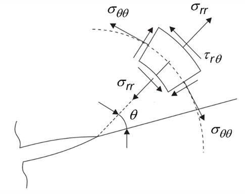
According to the MTS criterion, a crack tends to extend to a radial direction corresponding to the maximum tangential stress (Figure 3.8: Stress near crack-tip in polar coordinates) on a finite circle around the crack-tip [1].
The tangential stress (
 ) near a crack-tip is given by:
where
 and
and  are the stress-intensity factors for mode-I and
mode-II, respectively.
are the stress-intensity factors for mode-I and
mode-II, respectively.The kink angle (in rad) corresponding to the maximum
 is given by:
The equivalent stress-intensity factor is determined as:
Specify the MTS option for equivalent SIF and kink angle by issuing these commands:
The MTS formulation is the default option.
Richard approximation functions
Richard et al. [2] proposed approximation functions to evaluate the equivalent SIF and kink angle in a mixed-mode (I + II + III) fracture situation:
With the following parameter values (default), these functions are in close agreement with the
 -criterion by Schollmann et al. [3]:
 = 1.155,
  = 1.0
= 1.0 = 140°,
  = -70°
The
 -criterion assumes that the crack grows perpendicular
to the maximum principal stress
-criterion assumes that the crack grows perpendicular
to the maximum principal stress  , which is a function of the near-crack-tip stresses
 ,
,  , and
, and  [3]. Check the reference
for more details.
[3]. Check the reference
for more details.Specify the Richard functions for equivalent SIF and kink angle via the following commands:
Note that since the parameters are customizable, you can specify values other than the default, as needed.
Pook criterion
For a mixed-mode fracture, the equivalent stress-intensity factor is evaluated as follows according to the Pook criterion [4]. The equivalent SIF (I + II) is calculated first, based on the formulation of MTS criterion. The kink angle is the same as in the MTS criterion.
The equivalent SIF (I + II + III) is then determined as:
where
 is Poisson’s ratio.
Specify the Pook criterion for equivalent SIF and kink angle via the following commands:
Empirical function
You can define define an empirical function for equivalent SIF based on customizable parameters
 and
and  .
.The empirical formulation can be combined with any of the available options (MTS / RICHARD) for the kink angle calculation. Specify the empirical function for equivalent SIF and kink angle via the following commands:


References
The following references are cited:
Erdogan, F. and G. C. Sih. On the Crack Extension in Plates under Plane Loading and Transverse Shear. ASME Journal of Basic Engineering. 85: 519-527 (1963).
Richard, H.A., Eberlein, A. and Kullmer, G. Concepts and experimental results for stable and unstable crack growth under 3D-mixed-mode-loadings. Engineering Fracture Mechanics. 174:10-20 (2017).
Schöllmann, M., Richard, H.A., Kullmer, G. and Fulland, M. A new criterion for the prediction of crack development in multiaxially loaded structures. International Journal of Fracture. 117:129-141 (2002).
Pook, L.P. Comments on fatigue crack growth under mixed modes I and III and pure mode III loading. Multiaxial fatigue. Eds. Miller, K.J. and Brown,M.W. ASTM International, 1985.
When a crack begins to grow, a new mesh is generated. To correctly predict crack-growth behavior, any external loading associated with the remeshing volume must be mapped to the new meshes from the old meshes. Boundary conditions not in the remeshing volume are maintained as initially defined.
Note: Unless otherwise specified, any reference to boundary conditions assumes that they are associated with the remeshing volume. To obtain a correct solution, therefore, ensure that they are properly applied.
Boundary-condition and loading topics covered here are:
- 3.3.1.5.1. Displacement Boundary Condition
- 3.3.1.5.2. Temperature Boundary Condition
- 3.3.1.5.3. Force Boundary Condition
- 3.3.1.5.4. General Surface-Traction Load
- 3.3.1.5.5. Normal Surface Pressure Load to New Crack Surfaces
- 3.3.1.5.6. Initial Strain
- 3.3.1.5.7. Initial Stress
- 3.3.1.5.8. Crack-Surface Traction Load Derived from Initial StressSpaceClaim
- 3.3.1.5.9. Enhancing Crack Surfaces with Cohesive Zone Elements
You can use nodes or element components to define initial boundary conditions; however, Mechanical APDL does not maintain them after remeshing. It is therefore best to avoid using those components for any purpose (such as applying new boundary conditions at later load steps) after crack-growth has begun.
SMART crack-growth analysis handles the following types of displacement boundary conditions:
Displacement boundary condition on a node
Generally, a node with applied displacement boundary condition is treated as a hard node (that is, it remains unchanged throughout the analysis). Therefore, the applied boundary condition remains the same as the user input through the solution.
Constant displacement boundary condition on a face
A constant value of a displacement boundary condition is applied to a surface in a continuous facet of element faces. The surface topology is maintained throughout the solution. If the mesh changes due to remeshing as the crack grows and the meshing topology changes, the displacement boundary condition value is carried to the new mesh from the old mesh. This method also covers the fixed boundary condition on a face.
Non-constant displacement boundary condition on a face
Similar to the constant displacement boundary condition, a non-constant value or the tabular load of a displacement boundary condition is applied to a surface in a continuous facet of element faces. The surface topology is maintained throughout the solution. If the mesh changes due to remeshing as the crack grows and the meshing topology changes, the displacement boundary condition is mapped to the new mesh from the old mesh.
A displacement boundary condition can even be applied to nodes with their nodal coordinate systems rotated in any preferred direction (specified via NROTAT, NMODIF, NANG, or NORA). The node rotations and boundary condition values are properly mapped during remeshing.
When the mesh changes as a result of remeshing, the temperature boundary condition is mapped to the new mesh from the old mesh. The temperature between elements is assumed to be continuous.
Define the temperature boundary condition via TUNIF,
BFUNIF, BF, or BFE.
Tabular input (via *DIM and
%tablename%) for the temperature boundary is also
supported.
SMART crack-growth analysis handles the following types of force boundary conditions:
Force boundary condition on a node
Generally, a node with an applied force boundary condition is treated as a hard node (that is, it remains unchanged throughout the analysis). Therefore, the applied boundary condition remains the same as the user input through the solution.
Force boundary condition on a face
SMART does not map any force boundary condition on a face but treats the face with the force boundary condition as a hard face (where the face and nodes remain unchanged throughout the analysis). SMART may, therefore, create additional constraints which could lead to remeshing failure.
SMART supports general surface-traction loading. Loads must be applied directly on element faces.
When a surface-traction load is applied to a surface (SF or SFE, with or without SFCONTROL), the surface topology is maintained throughout the analysis.
If any part of the mesh changes because of crack-growth, the surface-traction loads are mapped from the old mesh to the new mesh, and the traction-control data from the old mesh also applies to the new one.
Within the traction-load surface, Mechanical APDL assumes a continuous traction load between elements, and that each surface has the same set of control data (introduced via SFCONTROL).
When a crack grows, the newly formed crack surfaces may be subjected to certain external loading such as surface pressure. Apply the crack-surface pressure load to the new crack surface, as follows:
CGROW,CSFL,PRES,,
Value |
where Value is the new constant
surface-pressure load to apply to the new crack surface for the current load
step.
To specify a table, enclose the table name within "%" characters
(%tablename%). Issue *DIM to
define the table. Only one table can be specified for a crack-growth set,
and time is the only primary variable supported.
CGROW,CSFL applies to both static and fatigue crack-growth simulation.
To apply stepped pressure loading in a fatigue crack-growth analysis, issue KBC,1. (The command is valid only for constant loading. For tabular loading, define a stepped load directly.)
When the mesh changes as a result of remeshing, the node- or element-based initial strains are mapped to the new mesh from the old mesh.
After remeshing, the existing initial strains are taken into account for the solution and for the fracture parameter calculation.
Define initial strain via this command:
| INISTATE,SET,DTYP,EPEL |
Generally, node-based initial strain offers better post-mapping accuracy than does element-based initial strain.
For more information, see Initial State in the Advanced Analysis Guide.
When initial stresses are present, the program first converts them internally to initial strains based on the material stiffness matrix at the first substep of the first load step, then calculates the fracture parameters via the initial-strain method. The initial strains are mapped from the old mesh to the new mesh during crack-growth.
Define initial stress via this command:
| INISTATE,SET,DTYP,STRE |
For more information, see Initial State in the Advanced Analysis Guide.
You can specify any residual (initial) stress as mesh-independent initial-stress data, and the program can convert that data to a traction load acting on the crack surfaces. As the crack grows, the program applies the traction to the new crack surfaces. The traction is applied as a step load for all substeps.
For more information, see:
When a crack grows, the crack surfaces can be enhanced using INTER204 3D 16-node cohesive interface elements to simulate a cohesive effect (for bonding tractions and to prevent crack-surface penetration). The cohesive elements are generated automatically during the first remeshing around the associated crack.
The process of generating the cohesive elements requires close topological matching between the upper and lower crack surfaces. Both surfaces should have the same number of vertices and edges on both sides, and each vertex/edge should have a counterpart on the opposite surface. Each pair of the topological entities should be as close as possible.
Generate INTER204 elements on a new crack surface as follows:
CGROW,CSFL,CZM,TB_CZM_ID,ESYS_ID |
where the cohesive zone material model parameters
are defined via TB_CZM_ID with
TB,CZM,,,,BILI, TB,CZM,,,,CEXP,
TB,CZM,,,,CLIN, or
TB,CZM,,,,REXP.
If the parameters are not specified or are set to zero, Mechanical APDL uses linear material behavior with a penalty slope to prevent surface penetration on the cohesive interface as the default cohesive model type (TB,CZM,,,,CLIN) . The program sets reasonable CZM parameters based on the solid elements around the crack fronts/surfaces.
The penalty stiffness for CLIN is determined by:

where:
 = characteristic element length around the crack (the
average element size) = characteristic element length around the crack (the
average element size) |
 = effective elastic modulus, calculated by: = effective elastic modulus, calculated by: |
 |
where subscripts  and and  denote upper and lower crack-surface materials,
respectively. denote upper and lower crack-surface materials,
respectively. |
The penalty stiffness for CLIN is evaluated at the reference temperature only. For temperature-dependent materials, define the CZM parameters (TB,CZM,,,BILI / CEXP / CLIN / REXP) to obtain an accurate result.
When TB,CZM,,,,FRIC / REXP is
applied and no valid local coordinate system (LCS) ID is specified
(ESYS_ID in
CGROW,CSFL,CZM,MAT_ID,ESYS_ID),
the program creates an internal LCS for CZM on crack surfaces. Information
about this internal LCS such as (ID, locations, and orientations) is
provided via echo messages. The LCS ID is assigned to the ESYS attribute of
the CZM elements inserted on crack surfaces; the program calculates and
displays tractions and separations in CZM elements in the element coordinate
system. The LCS is crucial for maintaining consistency in CZM during
remeshings.
When neither FRIC or REXP is specified, a valid
ESYS_ID in the CGROW,CSFL
command applies, although no internal LCS is created when
ESYS_ID is invalid or unavailable.
When INTER204 elements are enhanced to a crack surface with pressure loads, Mechanical APDL accounts for the contributions from both the cohesive tractions and pressure loads during fracture-parameter calculations.
When applying predefined pressures to a crack surface, and no pressures
are defined for the new open crack surface
(CGROW,CSFL,PRES), a fine mesh around the original crack
front is recommended. Issue
CGROW,RMCO,ESIZE,Par1,COMP,Par2,
where Par1 is the expected mesh size and
Par2 is the node-component name of the crack
front. (See CGROW,RMCO,ESIZE).
If a crack has existing cohesive zone elements on its surfaces, enable crack-surface loading (CGROW,CSFL,CZM) for the associated crack. All existing cohesive zone elements are maintained during remeshing.
If you enable crack-surface loading, Mechanical APDL detects the element type, material model, and element coordinate system for cohesive zone elements attached to the crack surfaces, then applies additional cohesive zone elements on new opened crack surfaces. (If your specified values are inconsistent with those expected by the program, a message appears and your values are not used; however, the program still applies cohesive zone surface loading to the crack surface using the values that it detects.)
For more information, see:
Fatigue crack-growth under
nonproportional loading is a complex phenomenon and can be difficult to analyze.
The varying mode mix occurring at different loading states, and the varying
stress ratio  , are among the challenges. SMART-based crack-growth analysis
supports nonproportional loading problems via cyclic loading
(CLOAD).
, are among the challenges. SMART-based crack-growth analysis
supports nonproportional loading problems via cyclic loading
(CLOAD).
The following topics for nonproportional fatigue loading are available:
When a crack is under nonproportional cyclic loading, SMART requires the history of the fracture-parameter calculations in intermediate steps of a loading cycle. A loading cycle can be introduced via CLOAD commands used in typical cyclic-loading analyses. Use CLOAD to define a loading cycle and repeat the cycle during the solution with loading tables:
CLOAD,DEFINE,BEGIN *DIM,_cycload1,TABLE,IMAX*DIM,_cycload2,TABLE,IMAXCLOAD,DEFINE,END
After applying a loading cycle, define the total number of cycles:[1]
CLOAD,CYCNUM,100 ! Total number of cycles
CLOAD commands are valid in a SMART-based fatigue crack-growth simulation only when applying nonproportional loading (CGROW,NPLOAD).
For more information, see Cyclic-Loading Analysis in the Advanced Analysis Guide.
SMART-based fatigue crack-growth offers options for defining the crack-propagation direction under nonproportional cycle loading, and for defining effective stress-intensity factors for fatigue-life calculation:
The crack-growth rate is typically dependent on the stress-intensity-factor range calculated from the maximum and minimum stress-intensity factor during a loading cycle.
With nonproportional loading, different fracture-modes typically have the corresponding minimum and maximum stress-intensity-factors occurring at different loading states:
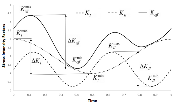
The stress-intensity-factor range drives fatigue crack-growth and must therefore be calculated from the history of a loading cycle. The following methods are available to introduce the stress ratio’s effect:
Effective stress-intensity-factor range method
The simplest method for calculating the stress-intensity-factor range is to use the difference between the maximum and minimum equivalent stress-intensity-factors at each crack-front node, determined by:

where:
 = equivalent stress-intensity-factor range at
each crack-front node = equivalent stress-intensity-factor range at
each crack-front node |
 = stress ratio at each crack-front
node = stress ratio at each crack-front
node |
 and and  = minimum and maximum equivalent
stress-intensity factors at each crack-front node,
respectively = minimum and maximum equivalent
stress-intensity factors at each crack-front node,
respectively |
The effective stress-intensity-factor range
at each crack-front node  is defined as

If there is no crack closure effect, the closure
parameter  , and thus
  .
.
At the end of each loading cycle analysis, the effective stress-intensity-factor range is used in the fatigue law as:

where  are the material parameters of fatigue
crack-growth law.
are the material parameters of fatigue
crack-growth law.
This command introduces the effective stress-intensity-factor range method in nonproportional fatigue problems:
CGROW,NPLOAD,METH,DKEFF |
This method overwrites any previously defined stress ratio (CGROW,FCG,SRAT). It works with any available fatigue law.
Stress-intensity-factor range method based on mode-separation
In some mixed-mode problems, mode-separation may be required to analyze complex nonproportional fatigue crack-growth. You can specify a stress-intensity-factor range based on mode-separation. The stress-intensity-factor range is formulated from the ranges of mode-separated stress-intensity factors at each crack front node as:

where:
 and and  = stress-intensity-factor ranges for mode I
and mode II at each crack-front node, respectively = stress-intensity-factor ranges for mode I
and mode II at each crack-front node, respectively |
 and and  = maximum stress-intensity-factors for mode I
and mode II at each crack-front node, respectively = maximum stress-intensity-factors for mode I
and mode II at each crack-front node, respectively |
 and and  = minimum stress-intensity-factors for mode I
and mode II at each crack-front node, respectively = minimum stress-intensity-factors for mode I
and mode II at each crack-front node, respectively |
The equivalent stress-intensity-factor
range  is formulated as a function of the mode-separated
stress-intensity-factor ranges
is formulated as a function of the mode-separated
stress-intensity-factor ranges  ,
,  , and
, and  as:
as:

where:
 = function for the equivalent
stress-intensity-factor formulation
(CGROW,SOPT,KEQV). = function for the equivalent
stress-intensity-factor formulation
(CGROW,SOPT,KEQV). |
 = nonproportional crack-growth direction
(CGROW,NPLOAD,DIRECTION) = nonproportional crack-growth direction
(CGROW,NPLOAD,DIRECTION) |
At the end of each loading-cycle analysis, the equivalent stress-intensity-factor range is used in the fatigue law as:

where:
 = stress ratio that you define
(CGROW,FCG,SRAT). Default = 0. = stress ratio that you define
(CGROW,FCG,SRAT). Default = 0. |
 = material parameters for the fatigue
crack-growth law. = material parameters for the fatigue
crack-growth law. |
This command introduces the stress-intensity-factor method based on mode-separation in nonproportional fatigue problems:
CGROW,NPLOAD,METH,DKMOD |
This method works with any available fatigue law.
Total effective stress-intensity-factor method
In special cases, the crack-growth rate can depend on a superposition of the minimum and maximum equivalent stress-intensity factors. You can use the summation of the maximum and minimum equivalent stress-intensity-factors at each crack front node as:

where:
 = superposed stress-intensity factor = superposed stress-intensity factor |
 and and  = minimum and maximum equivalent
stress-intensity factors, respectively = minimum and maximum equivalent
stress-intensity factors, respectively |
At the end of each loading-cycle analysis, the superposed stress-intensity factor is used in the fatigue law as:

where:
| = stress ratio that you define
(CGROW,FCG,SRAT). Default = 0. |
| = material parameters for the fatigue
crack-growth law. |
This command introduces the total effective stress-intensity-factor method in nonproportional fatigue problems:
CGROW,NPLOAD,METH,TKEFF |
This method works with any available fatigue law.
Total stress-intensity-factor method based on mode-separation
Also in special cases, the crack-growth rate can depend on a superposition of the minimum and maximum stress-intensity-factors. You can use the summation of the maximum and minimum mode-separated stress-intensity factors at each crack-front node as:

where  and
and  are the superposed stress-intensity factors for
mode I and mode II, respectively.
are the superposed stress-intensity factors for
mode I and mode II, respectively.
The equivalent stress-intensity-factor range is formulated as a function of the superposed stress-intensity-factor ranges as:

where:
 = function for the equivalent
stress-intensity-factor formulation.
(CGROW,SOPT,KEQV). = function for the equivalent
stress-intensity-factor formulation.
(CGROW,SOPT,KEQV). |
 = nonproportional crack-growth direction
(CGROW,NPLOAD,DIRECTION). = nonproportional crack-growth direction
(CGROW,NPLOAD,DIRECTION). |
At the end of each loading-cycle analysis, the superposed stress-intensity factor is used in the fatigue law as:

where:
| = stress ratio that you define
(CGROW,FCG,SRAT). Default = 0. |
| = material parameters for the fatigue
crack-growth law. |
This command introduces the total stress-intensity-factor method based on mode-separation in nonproportional fatigue problems:
CGROW,NPLOAD,METH,TKMOD
You can combine this method with your own stress-ratio input (CGROW,FCG,SRAT).[2]It works with any available any fatigue law.
The varying mode mixity occurring during a nonproportional loading cycle makes it difficult to predict crack-growth direction. SMART-based fatigue crack-growth offers the following methods for determining the crack-growth direction:
Maximum-load method
This method determines the angle based on
the mode mix at the instant when the equivalent stress-intensity
factor is maximum ( ). The crack-propagation direction is determined by
the angle formulation, a function of the stress-intensity factors
). The crack-propagation direction is determined by
the angle formulation, a function of the stress-intensity factors
 ,
,  , and
, and  at each crack-front node:

where  is the function for the crack-propagation-direction angle
formulation (CGROW,SOPT,KANG).
is the function for the crack-propagation-direction angle
formulation (CGROW,SOPT,KANG).
This command determines the crack-growth angle using the maximum-load method in nonproportional fatigue problems:
CGROW,NPLOAD,DIRECTION,KMAX |
Minimum-load method
This method determines the angle based on
the angle calculation at the instant when the equivalent
stress-intensity factor is minimum ( ). The crack-propagation direction is determined by
the angle formulation, a function of the stress-intensity factors
). The crack-propagation direction is determined by
the angle formulation, a function of the stress-intensity factors
 ,
,  , and
, and  at each crack-front node:

where  is the function for the
crack-propagation-direction angle formulation
(CGROW,SOPT,KANG).
is the function for the
crack-propagation-direction angle formulation
(CGROW,SOPT,KANG).
This command determines the crack-growth angle using the minimum-load method in nonproportional fatigue problems:
CGROW,NPLOAD,DIRECTION,KMIN |
Local kink-tip stress-intensity-factors method
This method uses the kink-tip stress-intensity factors:[14]

where:
 and and  = kink-tip stress intensity-factors at each
crack-front node = kink-tip stress intensity-factors at each
crack-front node |
 = local crack angles at each crack-front
node = local crack angles at each crack-front
node |
 = solution time = solution time |
and the different local crack angles of and the solution time, at each crack-front node.
The kink-tip stress-intensity-factor ranged is determined via:

where:
 = nodal kink-tip stress-intensity-factor range
at each crack-front node = nodal kink-tip stress-intensity-factor range
at each crack-front node |
 and and  = kink-tip stress-intensity factors at the
minimum and maximum load points at each crack-front node,
respectively, where = kink-tip stress-intensity factors at the
minimum and maximum load points at each crack-front node,
respectively, where  and and  are located in the loading cycle at each
crack-front node (as shown in Figure 3.9: Nonproportional Loading Example) are located in the loading cycle at each
crack-front node (as shown in Figure 3.9: Nonproportional Loading Example) |
Although maximization of  is a good agreement with simple experimental test
sets, a better approach is the maximization of a coupled
function:
is a good agreement with simple experimental test
sets, a better approach is the maximization of a coupled
function:

where  is a fitting parameter controlling the weight of
the function (default = 0.5). The angle at which the
crack-propagation direction is determined, for which
is a fitting parameter controlling the weight of
the function (default = 0.5). The angle at which the
crack-propagation direction is determined, for which  becomes the maximum, is:

This command determines the crack-growth angle using the local kink-tip stress-intensity-factor method in nonproportional fatigue problems:
CGROW,NPLOAD,DIRECTION,KLOC,ParW |
Note that this option is only supported when the kink angle calculation is based on MTS criterion (CGROW,SOPT,KANG,MTS).
Fatigue crack growth under spectrum loading is a common occurrence, and structures operating under mission conditions are typically subjected to complex spectrum loading. It is crucial to simulate such scenarios accurately to predict fatigue life. To simplify spectrum loading, cycle-counting techniques (such as rainflow counting, range-pair counting, and racetrack counting) are often used.
This figure illustrates loading in one pass (primary cycle) of a complex spectrum and its simplification via some cycle-counting method:
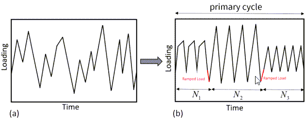
You can use the SMART method to analyze fatigue crack growth for a given spectrum loading. SMART requires simplified spectrum loading (shown by (b) in the figure) as input. SMART does not perform any conversion of a complex load-time history data to a simplified spectrum.
The following topics offer detailed usage information for spectrum fatigue loading:
When a crack model is subjected to cyclic loading containing several subcycles (shown by (b) in the figure), SMART calculates the fracture parameters at each time point of a subcycle. A complete spectrum loading (primary cycle) consisting of multiple subcycles can be introduced via a set of CLOAD commands for a multicycle analysis. (For more information, see Cyclic-Loading Analysis in the Advanced Analysis Guide.)
Example 3.3: Defining a Cyclic-Loading Table for SMART
CLOAD,DEFINE,BEGIN
*DIM,_cycload1,TABLE,4 ,2
CLOAD,DEFINE,END
The method can apply to proportional or nonproportional loading scenarios.
For proportional loading, the cyclic-loading table must contain the information for the maximum load and the number of cycles for every subcycle.
The zeroth, first, and second dimensions specify the time, load and number of cycles, respectively, for every subcycle in a primary cycle.
To define a proportional loading, every subcycle has two entries in the zeroth and first dimensions of the table. The first entry marks zero time and zero load. The second time entry specifies the time period for each subcycle. The second load entry marks the maximum load in the subcycle. The number of cycles for each subcycle is marked in the second dimension of the table.
Example 3.4: Specifying a Proportional Cyclic-Loading Table for SMART
CLOAD,MSUB,2          ! 2 subcycles

! Time values
_cycload1(1,0) = 0.   ! time must start at 0
_cycload1(2,0) = t1
_cycload1(3,0) = 0    ! time must start at 0 for every subcycle
_cycload1(4,0) = t2
! Load values
_cycload1(1,1) = 0.
_cycload1(2,1) = p1   ! first proportional load value
_cycload1(3,1) = 0
_cycload1(4,1) = p2   ! second proportional load value
! Number of cycles
_cycload1(1,2) = n1   ! number of cycles of the first load
_cycload1(3,2) = n2   ! number of cycles of the second load
Although every subcycle has two entries, the analysis is performed only at the time-point with the load value for each subcycle.
The default stress ratio for each subcycle is zero. Any non-zero stress
ratio for the subcycles can be specified
(CGROW,FCG,SRAT,%_tab_srat%).
The time-dependent table _tab_srat contains the
stress-ratio information for the complete primary cycle.
Example 3.5: Specifying the Stress Ratio for the SMART Proportional Cyclic-Loading Table
*DIM,_tab_srat,TABLE,3,1,,TIME

! Time values
_tab_srat (1,0) = 0.
_tab_srat (2,0) = t1
_tab_srat (3,0) = t1+t2

! Stress ratio values
_tab_srat (1,1) = 0.
_tab_srat (2,1) = R1  ! stress ratio for first subcycle
_tab_srat (3,1) = R2  ! stress ratio for second subcycle

! CGROW command for stress ratio
CGROW,FCG,SRAT,%_tab_srat%
For multicycle cyclic loading
(CLOAD,MSUB,n) where only
single loading applies in each subcycle, the program activates proportional
loading automatically.
Similarly, the spectrum cyclic-loading method can be used for nonproportional loading. In this case, the analysis of each subcycle involves solutions at more than one load value. Every subcycle must have the same loads at the start and end time points. If ramped loads exists between subcycles, add them by setting the subcycle number to -1.
Example 3.6: Specifying a SMART Nonproportional Cyclic-Loading Table
CLOAD,DEFINE,BEGIN
*DIM,_cycload1,TABLE,10 ,2
CLOAD,DEFINE,END

CLOAD,MSUB,4

! Time values
_cycload1(1,0) = 0.   ! time must start at 0
_cycload1(2,0) = t11
_cycload1(3,0) = t12
_cycload1(4,0) = 0.   ! time must start at 0 for every subcycle
_cycload1(5,0) = t21
_cycload1(6,0) = 0    ! time must start at 0 for every subcycle
_cycload1(7,0) = t31
_cycload1(8,0) = t32
_cycload1(9,0) = 0.   ! time must start at 0 for every subcycle
_cycload1(10,0) = t41


! Load values
_cycload1(1,1) = 0
_cycload1(2,1) = p11   ! first subcycle load value
_cycload1(3,1) = 0
_cycload1(4,1) = 0     ! ramped load begins
_cycload1(5,1) = p21   ! ramped load ends
_cycload1(6,1) = p31   ! second subcycle load value, p31=p21
_cycload1(7,1) = p32   ! second subcycle load value
_cycload1(8,1) = p33   ! second subcycle load value, p33=p31
_cycload1(9,1) = p41   ! ramped load begins, p41=p33
_cycload1(10,1) = 0    ! ramped load ends

! Number of cycles
_cycload1(1,2) = n1   ! number of cycles of the first load
_cycload1(4,2) = -1   ! ramped load, ignored in SMART
_cycload1(6,2) = n2   ! number of cycles of the second load
_cycload1(9,2) = -1   ! ramped load, ignored in SMART
Ramped loads are not included in the fatigue calculation for spectrum loading.
Options are available for specifying nonproportional-loading and crack-growth direction (CGROW,NPLOAD). If not specified, the program uses the default options.
For multicycle cyclic loading
(CLOAD,MSUB,n) where more than
single loadings exist in the subcycles (not counting ramped loads), the
program activates nonproportional loading automatically.
In SMART spectrum loading, individual cycles are not repeated in the subcycles in order to reduce computational cost. Instead, the program calculates damage accumulation from cyclic fatigue loading in each subcycle using the Palmgren-Miner linear damage rule:

where:
 = index of a crack-front node = index of a crack-front node |
 = nodal damage from all of the subcycles of one
primary cycle = nodal damage from all of the subcycles of one
primary cycle |
 = number of subcycles = number of subcycles |
 = repeat number of an individual cycle for the = repeat number of an individual cycle for the
ith subcycle |
At the end of each subcycle,  is calculated at each crack-front node (via a proportional
or nonproportional solution) using the specified fatigue law.
is calculated at each crack-front node (via a proportional
or nonproportional solution) using the specified fatigue law.
 represents the number of cycles of the
ith subcycle required to cause damage of unit
crack extension:

After  is evaluated via the Palmgren-Miner rule, the number of
primary cycles
is evaluated via the Palmgren-Miner rule, the number of
primary cycles  (where one primary cycle is shown by (b) in the figure) required to
propagate the crack by
(where one primary cycle is shown by (b) in the figure) required to
propagate the crack by  units is determined by:

The crack increment at the crack-front is determined for the cycle increment via the crack-growth law:

The default method for obtaining the crack kink angle at a node at the end of each primary cycle involves calculating a weighted average of the kink angles from each individual subcycle (CGROW,SOPT,SPLO,WEIG):

Another approach for specifying the kinking angle in crack propagation involves using the kink angle from the dominant step, where the maximum damage is created (CGROW,SOPT,SPLO,DMAX):

Similarly, the average stress ratio for a primary cycle  is calculated as a weighted average of stress ratios of
every individual subcycle:
is calculated as a weighted average of stress ratios of
every individual subcycle:

The average stress-intensity-factor range at a crack-front node for each
primary cycle can be obtained via a Newton-Raphson iteration of specified
fatigue law function (Paris’
Law, Walker Equation, Forman Equation, NASGRO Equation). The average quantities
 and
and  should satisfy the fatigue law as:

where  are the fatigue law parameters.
The following output quantities are available (PRCINT or *GET) at the end of each primary cycle of spectrum loading:
| Label | Quantity | Meaning |
|---|---|---|
| DLTK |  | Average stress-intensity-factor range |
| R |  | Average stress ratio |
| DLTN |  | Primary cycle increment number |
| DLTA |  | Crack-growth increment |
Fracture parameter values (such as  ,
,  , and
, and  ) are accessible at each solution substep (via
PRCINT or *GET). The crack-growth
solution (DLTK, R, DLTN, DLTA and KANG) for each primary cycle are available
at the substep corresponding to the last time-point of that primary
cycle.
) are accessible at each solution substep (via
PRCINT or *GET). The crack-growth
solution (DLTK, R, DLTN, DLTA and KANG) for each primary cycle are available
at the substep corresponding to the last time-point of that primary
cycle.
When a crack begins to grow, SMART refines the mesh around the new crack front for better accuracy to accommodate the singularity of the crack tip. Without suitable coarsening of the mesh behind the crack front, the mesh around the crack front may be excessively fine.
In such cases, three mesh-coarsening options (specified via CGROW) are available:
Conservative (default) – Provides the least mesh-coarsening, resulting in a larger number of nodes and elements after a substantial amount of crack-growth. This option generally offers the best remeshing success rate.
CGROW,RMCONT,COARSE,CONS Moderate – Performs a moderate reduction in the number of nodes and elements, and offers a good remeshing success rate.
CGROW,RMCONT,COARSE,MODE Aggressive – Quickly coarsens the mesh in the region behind crack front, offering the largest reduction in the number of nodes and elements after a substantial amount of crack-growth. This option is the most likely one to cause remeshing failure.
CGROW,RMCONT,COARSE,AGGR
When multiple cracks exist, the specified mesh-coarsening option applies to the last identified crack.
When a crack begins to grow, SMART uses the mesh around the crack front to determine the crack-increment size for the robustness and accuracy of the crack-growth analysis.
If your model has a relatively small crack (and a correspondingly fine mesh) at the start of the solution, SMART may require a very small crack increment. Using that initial crack-growth increment throughout the analysis, however, can result in an excessive number of crack-growth increments and solution steps. As the crack propagates during the solution process, a very small crack-growth increment may become unnecessary and a larger increment may be more desirable.
Conversely, suppose that a crack front approaches a critical regime (such as a boundary or interface), requiring a finer mesh around the crack front for the sake of parameter-calculation accuracy. In that case, a smaller crack-growth increment may again be necessary.
For such scenarios, two command options (specified via CGROW) are available for controlling the crack-increment size:
Direct element-size control
This command controls the reference-element size (
ESIZE) that SMART uses to determine the crack-growth increment at each solution step:CGROW,RMCONT,ESIZE, ValueThe command offers a static crack-increment size with a constant value, or a dynamic crack-increment size as a function of solution time with a table data. Only one table can be specified for a crack-growth set, and time is the only valid primary variable.
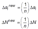
Crack-growth increment-multiplier control
Use this method to adjust the crack-increment control parameter
 , where
  . (
. ( is the reference-element size at the initial crack
front.) By default, the crack increment is proportional to the
reference-element size
is the reference-element size at the initial crack
front.) By default, the crack increment is proportional to the
reference-element size ESIZEat the substep.Issue this command to control the crack increment:
CGROW,RMCONT,CMULT The command's crack-front element-size multiplier controls this function:
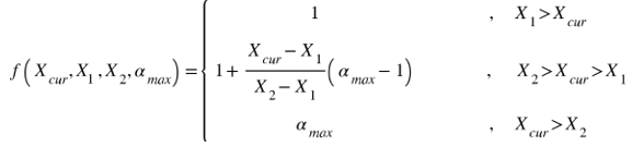
The control method can be a function of the solution time, accumulated maximum crack extension, or number of remeshings:
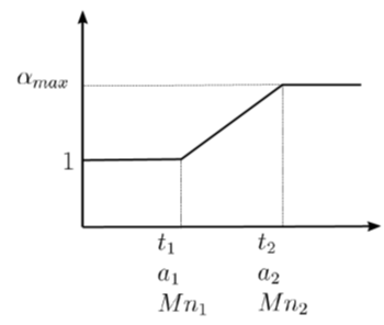
Solution time – CGROW,RMCONT,CMULT,TIME,
Value ,
,Value ,
,Value
The control parameter is a function of the solution time:
 , where
  are the input value of the solution time at the
beginning, the current time, the input value of the time at the end, and
the user input for the maximum value of the multiplier,
respectively.
are the input value of the solution time at the
beginning, the current time, the input value of the time at the end, and
the user input for the maximum value of the multiplier,
respectively.Crack length – CGROW,RMCONT,CMULT,CEMX,
Value ,
,Value ,
,Value
The control parameter is a function of the accumulated maximum crack extension:
 , where
  are the input value of the crack length at the
beginning, the current crack length, the input value of crack length at
the end, and the user input for the maximum value of the multiplier,
respectively.
are the input value of the crack length at the
beginning, the current crack length, the input value of crack length at
the end, and the user input for the maximum value of the multiplier,
respectively.Number of remeshings – CGROW,RMCONT,CMULT,RMNU,
Value ,
,Value ,
, Value
The control parameter is a function of the number of remeshings:
 , where
  are the input value of number of the remeshing number
at the beginning, the current remeshing number, the input value of
number of the remeshing number at the end, and the user input for the
maximum value of the multiplier, respectively.
are the input value of number of the remeshing number
at the beginning, the current remeshing number, the input value of
number of the remeshing number at the end, and the user input for the
maximum value of the multiplier, respectively.
If the maximum multiplier value  > 1, the crack increments increase; if < 1, the crack increments decrease. If the current variable
< beginning variable of the function, Mechanical APDL uses 1; if the current
variable > end variable of the function, the program uses the maximum
multiplier value:
> 1, the crack increments increase; if < 1, the crack increments decrease. If the current variable
< beginning variable of the function, Mechanical APDL uses 1; if the current
variable > end variable of the function, the program uses the maximum
multiplier value:
If the input is tabular data (CGROW,RMCONT,CMULT,
TABLE,%tablename%), the table containing the data
controls the parameter directly. You can specify one table per crack-growth set,
and time is the only valid primary variable.
Accurate parameter calculation in a SMART crack-growth simulation requires a sufficiently fine mesh around the crack front.
Because a very fine mesh for the entire remeshing zone leads is computationally expensive, SMART remeshing uses a fine mesh around the crack front and a coarse mesh in the far field. This approach can, however, lead to accuracy loss in special zones such as boundaries, interfaces, voids, and holes. If your model has such areas where the mesh must be conserved or controlled, options (specified via CGROW,RMCONT,ESIZE) are available to control the element size in the remeshing zone:
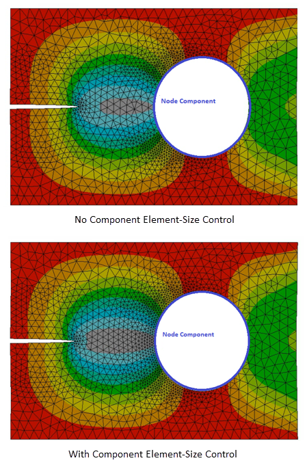
Component-based element-size control
To control the reference element size by introducing a component that you have specified for SMART crack-growth analysis, issue this command:
CGROW,RMCONT,ESIZE, Value,COMP,ComponentNameThe command offers a constant element size with a constant value or a dynamic element-size control as a function of solution time using tabular data. Time is the only valid primary variable for the table. The component can be an element or a node component. Although remeshing does not maintain the component node or element numbers, SMART uses the locations after the first remeshing. If
Valueis not specified or is zero, the averaged element size is used. If the command is issued for the same component more than once, SMART uses the last element size.Element-based element-size control
To control the reference element size by introducing an element number in the initial mesh that you have specified for SMART crack-growth analysis, issue this command:
CGROW,RMCONT,ESIZE, Value,ELEM,ELEMIDThe command offers a constant element size with either a constant value or a dynamic element-size control as a function of solution time using tabular data. Time is the only valid primary variable for the table. Although remeshing does not maintain the element numbers, SMART uses the location after the first remeshing. If
Valueis not specified or is zero, the averaged element size is used. If the command is issued for the same element more than once, SMART uses the smallest element size.Node-based element-size control
To control the reference element size by introducing a node number in the initial mesh that you have specified for SMART crack-growth analysis, issue this command:
CGROW,RMCONT,ESIZE, Value,NODE,NODEIDThe command offers a constant element size with either a constant value or a dynamic element-size control as a function of solution time using tabular data. Time is the only valid primary variable for the table. Although remeshing does not maintain the node numbers, SMART uses the location after the first remeshing. If
Valueis not specified or is zero, the averaged element size is used. If the command is issued for the same node more than once, SMART uses the smallest element size.
Fracture mechanics deals with cracks (defects), and a singularity always exists around a crack front. The finite element solution therefore always depends on the element sizes, especially around the crack front. To ensure consistent results throughout the crack-growth process, maintain a reasonable crack-front element size and crack-growth increment. The crack-growth increments are usually of the order of the average element size at the crack front.
You can specify the maximum crack-growth increment
(damax) as an absolute value or a multiple of the
reference-element size (ESIZE) at the crack front:
damax = m *
ESIZE (Default: m =
1.5)
The minimum crack-growth (damin) is specified in a
similar way. (Default: damin = 0). To explore options
for specifying damin and
damax, see CGROW,SOPT.
You can also control ESIZE at the crack front as
the crack grows via CGROW,RMCONT,CMULT and
CGROW,RMCONT,ESIZE.
The crack-growth calculation occurs in the solution phase after stress calculation. The fracture parameter is calculated first, followed by the crack extension according to the crack-growth method:
If using the fatigue crack-growth life-cycle (LC) method:
CGROW,FCG,METH,LCThe crack-growth rates
 are first evaluated at all crack-front nodes according
to the specified crack-growth law. Crack-growth rate at node i:
are first evaluated at all crack-front nodes according
to the specified crack-growth law. Crack-growth rate at node i:where
 is the stress-intensity factor,
  is the stress ratio, and
  is the temperature.
The
 at the node with the maximum crack-growth rate
 is set equal to
  :
:The cycle increment
 is calculated as:
The
 at the remaining nodes is determined by:
If using the fatigue crack-growth cycle-by-cycle (CBC) method:
CGROW,FCG,METH,CBCCGROW,FCG,DN,ΔNFor this method,
 is a user-specified cycle increment.
The preliminary
 at the crack-front nodes is calculated for the cycle
increment using the crack-growth law:
at the crack-front nodes is calculated for the cycle
increment using the crack-growth law:If the maximum increment
 exceeds the maximum-limit
  , the program scales the
  and
and  values down by a factor of
1/
values down by a factor of
1/nso that the new maximum is <  . Here,
  is a natural number.
If the preliminary
is <  , the program scales the
  and values up by a factor of
  so that the new maximum is closer to
  .
.Scaling up or down does not alter the crack-growth rate at any crack-front node.
If using static crack-growth:
If the maximum equivalent stress-intensity factor
 at the crack front is greater than the specified
criterion, the crack is set to grow. The node with the maximum
at the crack front is greater than the specified
criterion, the crack is set to grow. The node with the maximum
 is assigned with a crack extension
  equal to the specified maximum limit
  .
.Crack increments at other nodes are evaluated as:


To specify the maximum crack-growth increment
(damax):
CGROW,SOPT,DAMX,Value,Option
If Option= ABSO (default):If Option= MULT:Default:
For mesh-coarsening (CGROW,RMCONT,COARSE), the default option (CONS) allows a maximum
value of up to
. For the moderate (MODE) and aggressive (AGGR) options,
can be extended up to
.


To specify the minimum crack-extension
increment (damin):
CGROW,SOPT,DAMN,Value,Option1,Option2
If Option1= ABSO (default):If Option1= MULT:
If Option2= 0 (default): Sets the crack extensionsbelow
as
.
If Option2= 1: Sets the crack extensionsbelow
as
.
Default:
By default, the program sets any crack extension <
to
. To change the default setting, specify a non-zero
value. Valid
values are between 0 and
.


When the fracture criterion is reached for the specified crack-growth type, the program determines the crack-growth increment and generates the new crack surfaces.
For an analysis involving multiple cracks, you can set different
and limits for individual cracks.
For a fatigue crack-growth analysis for multiple cracks, the program maintains
the cycle increment  at a substep for all cracks
(CGROW,SOPT,SCN) by default. The program selects
at a substep for all cracks
(CGROW,SOPT,SCN) by default. The program selects
 such that
  values at all cracks are within their respective
 limits. Crack-extension at a node is determined via:

For a static crack-growth analysis involving multiple cracks, the crack node
with the maximum stress-intensity factor  (among all cracks) is identified. Crack extension at that
node, at crack
(among all cracks) is identified. Crack extension at that
node, at crack j for example, is assigned the
corresponding value (that is,  ). Crack extensions at other nodes related to any crack are
determined as:
). Crack extensions at other nodes related to any crack are
determined as:

To control how the program handles small crack extensions at any crack, use
the  options (CGROW,SOPT,DAMN).
SMART supports static or fatigue crack-growth analyses:
The CGROW command defines all necessary crack-growth-calculation parameters.
Define a set number for this crack-growth calculation:
CGROW,NEW,SETNUMBERSpecify the crack-calculation ID (created when you defined the fracture-parameter calculation set) to use as the fracture criterion:
CGROW,CID,IDSet the crack-growth method to SMART:
CGROW,METHOD,SMART,REMESpecify the fracture criterion:
CGROW,FCOPTION,when the fracture parameter is only a constant,Par1,Par2or, when fracture parameters are more than just a constant,
TB,CGCR,MAT_ID,,,OptionCGROW,FCOPTION,MTAB,MAT_ID,CONTOURSet the crack-growth time-stepping controls:
CGROW,DTMAX,MAX_TIME_STEPCGROW,DTMIN,MIN_TIME_STEPSpecify maximum and minimum crack-growth increments in a step:
CGROW,SOPT,DAMX,Value,Option1CGROW,SOPT,DAMN,Value,Option1,Option2Stop the crack analysis as needed:
CGROW,STOP,CEMX,MAX_CRACK_EXTThe command stops the analysis when the crack extension for any crack-front node reaches the maximum value specified.
This command stops the analysis when the crack extension reaches free boundary:
CGROW,STOP,FBOUThis command stops the analysis when the maximum equivalent stress-intensity factor at the crack front exceeds the specified limit:
CGROW,STOP,KMAX,MAX_SIF
Large Time Steps and Fracture Parameters — A crack-growth condition is based on whether the fracture criterion is met along the crack-front nodes; therefore, a large time step may result in significant over-prediction of the fracture parameters (and therefore the load-carrying capacity of the structures). A large time step can also cause over-prediction in the solution when crack-growth becomes unstable. In both cases, try using a small minimum time DTMIN.
Define a set number for this crack-growth calculation:
CGROW,NEW,SETNUMBERSpecify the crack-calculation ID (created when you defined the fracture-parameter calculation set) to use as the fracture criterion:
CGROW,CID,IDSet the crack-growth method to SMART:
CGROW,METHOD,SMART,REMESpecify either the life-cycle (LC) or cycle-by-cycle (CBC) method for the fatigue crack-growth calculation:
CGROW,FCG,METH,LCorCBCIf using the CBC method, also specify the cycle increment to use in a calculation step:
CGROW,FCG,DN,INCREMENTSpecify the fatigue crack-growth model and parameters:
TB,CGCR,MAT_ID,,,OptionCGROW,FCOPTION,MTAB,MAT_ID,CONTOURSpecify the stress ratio:
CGROW,FCG,SRAT,VALUESpecify maximum and minimum crack increments in a step:
CGROW,SOPT,DAMX,Value,Option1CGROW,SOPT,DAMN,Value,Option1,Option2Specify maximum and minimum crack increment in a step:
CGROW,FCG,DAMX,MAX_INCREMENTCGROW,FCG,DAMN,MIN_INCREMENTStop the crack analysis as needed:
CGROW,STOP,CEMX,MAX_CRACK_EXTThe command stops the analysis when the crack extension for any crack-front node reaches the maximum value specified.
This command stops the analysis when the crack extension reaches free boundary:
CGROW,STOP,FBOUThis command stops the analysis when the maximum equivalent stress-intensity factor at the crack front exceeds the specified limit:
CGROW,STOP,KMAX,MAX_SIFIf multiple cracks are defined, specify the type of load cycles:
A single cycle count for multiple cracks (default) –
CGROW,SOPT,SCNA separate cycle count for each crack –
CGROW,SOPT,MCNThis option is available only in cases where a separate loading is applied to each crack.
Specify the threshold stress-intensity-factor range:
CGROW,FCG,DKTH,/VALUE,blank or MINMAX/AVERIf the last parameter is unspecified (default), the program ensures zero crack extension at any crack-front node where the equivalent stress-intensity-factor range (ΔK) is below the threshold (
VALUE). This setting allows partial growth to occur at the crack front.If the last parameter is MIN, MAX, or AVER, the program enforces zero crack extension for the entire crack front when the minimum/maximum/average ΔK at the crack front is below the threshold (
VALUE). If the criterion is satisfied, crack-growth is arrested completely even though ΔK at some nodes may exceed the threshold. This setting does not allow partial growth to occur.Do not issue this command when crack-growth is based on the NASGRO equation (v. 3 or v. 4). The equation incorporates the threshold stress-intensity-factor range inherently.
Also see Example: Fatigue Crack-Growth Analysis Using SMART.
SMART supports 3D crack-growth only.
SMART is used with SOLID187 only.
Nodes and elements components are not maintained after the remeshing process, unless you set the component's update key option (CM,,,,
KOPT) to active (CM,,,,1). It is important to note that this option is applicable only to solid element components and surface node components.Overlapping between multiple surface node components can cause re-meshing failure. Crack-surface node components (defined using CINT,SURF) are automatically updated during definition, so it is important to ensure that there is no overlap when defining multiple surface node components, especially between the surface components and the crack-surface components.
Material behavior is assumed to be linear elastic isotropic, with only one material in the crack-growth domain.
Plasticity effects and nonlinear geometry effects are not considered.
When the crack grows to the point of breaking the structural component apart, all solution results are set to zero and no crack-front information is reported.
SMART supports bonded, no-separation, frictionless, rough, and frictional contact options with CONTA174 and TARGE170 when they remain outside the remeshing zone during the simulation. (SMART does not support any contact element inside the remeshing zone.)
Due to the renumbering of elements and nodes in the remeshing zone, SMART crack-growth simulation does not support tabular loads defined via table parameters having ELEM and/or NODE as primary variables.
For models with multiple cracks, crack merging is not supported. When two cracks grow into each other, a meshing error is likely to occur, stopping the solution process due to meshing failure.
SMART does not account for both a pressure and a force load on the same face. In such cases, the pressure load is overwritten.
Coupling commands (including CP, CPCYC, CPINTF, CPLGEN, CPMERGE, CPSGEN) are not supported.
It is possible to define or modify boundary conditions applied on elements and/or nodes after the initial load step or during a restart process. However, if remeshing occurs (where positions of nodes or elements change), use caution when updating the boundary conditions applied on those elements and/or nodes.
Any rotations of nodal coordinate systems are maintained inside the remeshing zone only if those nodes are associated with a displacement boundary condition. Otherwise, the nodal rotations are not maintained during remeshing, and any new node is set with the default nodal coordinate system.
After the first load step or during a restart, you cannot define a new crack growth (CGROW, NEW) or switch between fracture criteria.
Function-based loads and tabular loads with time as an independent variable are not supported for fatigue crack growth. Such loads can lead to number-of-substeps (NSUBST) or time-step-size-dependent (DELTIM) results.
When specifying an element coordinate system (ESYS) for existing CZM elements on crack surfaces (TB,CZM), the element normal must point away from the primary crack surface and toward the secondary crack surface (that is, from
Par1toPar2, wherePar1andPar2are defined via CINT,SURF,Par1,Par2).Consistent use of ESYS for CZM elements on the original and new crack surfaces is important for rebuilding CZM elements, mapping local variables, and displaying elements results. Check ESYS for CZM elements (/PSYMB,ESYS,1) after each remeshing, especially in analyses involving curved crack surfaces or kinked crack-growth paths.
A critical component in the SMART framework is remeshing as a result of crack-growth. When a crack is growing, however, the crack profile can become very complex even for a simple initial crack geometry; therefore, be aware that remeshing is not always successful. Try the following if you encounter remeshing failure:
Adjust the initial mesh. A very large mesh-size difference between adjacent elements can sometimes cause remeshing failure.
Try a different number of contours for fracture-parameter calculation. SMART uses the number of contours as a reference to determine the remeshing volume. Try using four to six contours.
Do not use surface-effect elements (SURF15
xxx) for loading purposes (including surface pressure) in the remeshing zone.
Use the following standard POST1 (/POST1) commands for postprocessing SMART crack-growth analysis results:
| Command | Purpose |
|---|---|
| ANDATA | Displays animated graphics data for nonlinear problems |
| ANTIME | Generates a sequential contour animation over a range of time |
| *GET | Retrieves a value and stores it as a scalar parameter or part of an array parameter |
| OUTRES | Output control |
| PLCINT | Plots the fracture-parameter (CINT) results data |
| PLDISP | Displays the displaced structure |
| PLESOL | Displays the solution results as discontinuous element contours |
| PLNSOL | Displays results as continuous contours |
| PLVECT | Displays results as vectors |
| PRCINT | Prints fracture parameters and crack-growth information |
| PRESOL | Prints element solution results |
| PRNSOL | Prints nodal solution results |
| PRVECT | Prints results as vector magnitude and direction cosines |
The nature of crack-growth simulation almost always implies many substeps and a correspondingly large results file. Take advantage of OUTRES to control output frequency, thereby reducing the size of the results file.
Example 3.7: Limiting SMART Results File Size via OUTRES
CINT (fracture-parameter) results are calculated and output at all load steps and substeps. Nodal and element solutions are output every five substeps. No other output (such as reaction force) is written to the results file.
OUTRES,ERASE
OUTRES,ALL,NONE
OUTRES,NSOL,5
OUTRES,ESOL,5
OUTRES,CINT,ALL
Geometry data, such as new mesh information generated by crack-growth remeshing, is not output to the results file at substeps without solution outputs, though remeshing may occur at that moment. Geometry data access for such substeps is linked to the last available results set. Therefore, given the OUTRES arguments shown in the example:
In cases where more precise information is necessary to track crack configuration and model deformation, OUTRES,ALL,ALL is a better option (at the cost of a larger results file).
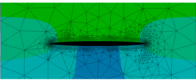
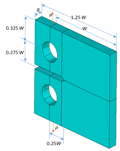
The following figure represents the model to be used in a SMART-based fatigue crack-growth simulation:
The fatigue calculation is based on Paris' Law. The numbers of cycles are obtained for various crack-growth increments and compared to the reference solution.
Following are the material properties, specimen dimensions, and loading:
| Material Properties | Geometry | Loading |
|---|---|---|
|
E = 2e5 MPa, Paris’ Law parameters: C = 2.29e-10 mm / (cycle · MPam · mmm/2) = 2.29e-10 1 / (cycle · MPa2), where m = 2 |
a = 46.6 mm W = 100 mm B = 12 mm |
P = 450 N Stress ratio: R = 0 |

The theoretical stress-intensity factor for a compact-tension specimen [1] is:

For the specified stress ratio R = 0 and under a constant load P, the
stress-intensity factor range for a crack length  is
is  . The number of cycles for a crack extension
  is estimated via Paris’ Law as
  . The values calculated are used as reference for validation of the
Mechanical APDL results.
. The values calculated are used as reference for validation of the
Mechanical APDL results.
The problem is solved in Mechanical APDL using the 3D SOLID187 element. Stress-intensity factors (SIFS) are defined for the fracture parameter, and SMART is used for the crack-growth analysis (CGROW,METHOD,SMART).
To impose a plane-strain condition, nodes at the front and back faces of the specimen are constrained through the out-of-plane direction.
The life-cycle (LC) method is used for the fatigue analysis with a maximum crack-growth increment of 0.5 mm. The number of cycles is obtained corresponding to crack extension in each substep.
This table compares the Mechanical APDL results with the reference results at the first
node of the crack-front nodes, where is the cumulative crack extension and  is the cumulative number of load cycles:
|
(mm) | Reference | Mechanical APDL | Ratio |
|---|---|---|---|
 of the First Node
(MPa.mm0.5) of the First Node
(MPa.mm0.5) | |||
| 0.497 | 32.534 | 32.421 | 0.997 |
| 0.997 | 32.987 | 33.016 | 1.001 |
| 1.497 | 33.454 | 33.615 | 1.005 |
| 1.992 | 33.932 | 33.917 | 1.000 |
| 2.490 | 34.416 | 34.420 | 1.000 |
| 2.982 | 34.917 | 34.734 | 0.995 |
| of the First Node: | |||
| 0.497 | 2051037 | 2065322 | 1.007 |
| 0.997 | 4057587 | 4068384 | 1.003 |
| 1.497 | 6008552 | 6000662 | 0.999 |
| 1.992 | 7883540 | 7877231 | 0.999 |
| 2.490 | 9720231 | 9713513 | 0.999 |
| 2.982 | 11483748 | 11495627 | 1.001 |
Following is the input file for the example fatigue crack-growth analysis using SMART:
/prep7

A = 46.6       	! crack length, mm
W = 100        	! width, mm
W1 = 125       	! total width, mm
H = 60         	! half height, mm
R = 12.5       	! radius of load circle, mm
E = 27.5       	! pin height, mm
S = 3          	! half width of notch, mm
D1 = 80        	! depth of notch, mm
D2 = 75        	! depth of notch, mm
B  = 12       	! thickness, mm

PF = 450 		! pin load, N

k,1,A
k,2,W
k,3,W,H
k,4,,H
k,5,(W-W1),H
K,6,(W-W1),S
k,7,,S
k,8,(W-D1),S
k,9,(W-D2)
k,10,,E
k,11,,E,E

k,20,W,-H
k,21,,-H
K,22,(W-W1),-H
k,23,(W-W1),-S
k,24,,-S
k,25,(W-D1),-S
k,26,(W-D2)
k,27,,-E
k,28,,-E,E

k,40,(W-D1),H
k,41,(W-D1),-H

circle,10,r,11,4,,8
l,1,2
l,2,3
l,3,40
l,40,4
l,4,5
l,5,6
l,6,7
l,7,8
l,8,9
l,9,1
l,4,12
l,16,7

circle,27,r,28,21,,8
l,20,41
l,41,21
l,21,22
l,22,23
l,23,24
l,24,25
l,25,26
l,26,1
l,2,20
l,24,33
l,29,21
l,8,40
l,25,41

al,9,10,11,40,17,18
al,41,35,36,9,37,29
al,12,19,8,7,6,5,20,16,40
al,34,38,24,23,22,21,39,30,41
al,38,33,32,31,39,28,27,26,25
al,13,19,1,2,3,4,20,15,14


et,1,187
type,1
mp,ex,1,200000 		! elastic modulus, MPa
mp,nuxy,1,0.33 		! Poisson's ratio

! Paris' Law Constants (units of delta-K in MPa.mm0.5, da/dN in mm/cycle)
C=2.29E-10
M=2

! Fatigue crack-growth law specification
tb,cgcr,2,,,PARIS
tbdata,1,C,M

esize,4
vext,all,,,0,0,-B
allsel,all

vmesh,all

asel,s,,,8
asel,a,,,18
asel,a,,,13
arefine,all,,,,1

asel,s,,,23
asel,a,,,24
asel,a,,,25
asel,a,,,26
asel,a,,,50
asel,a,,,51
asel,a,,,52
asel,a,,,53
nsla,s,1

*get,numnode,node,0,count,,,
f,all,fy,PF/numnode
allsel,all

asel,s,,,33
asel,a,,,34
asel,a,,,35
asel,a,,,36
asel,a,,,39
asel,a,,,40
asel,a,,,41
asel,a,,,42
nsla,s,1

*get,numnode,node,0,count, , ,
f,all,fy,-PF/numnode
allsel,all

lsel,s,,,49
nsll,s,1
d,all,uy,0
allsel,all

lsel,s,,,74
lsel,a,,,90
nsll,s,1
d,all,ux,0
allsel,all

! plane strain, Uz constrained at front and back faces
nsel,s,loc,z,0
nsel,a,loc,z,-B
d,all,uz,0
allsel,all

! crack-front-nodes component
nsel,s,loc,x,a
nsel,r,loc,y,0
nlist
cm,crack1,node
allsel,all

! upper crack-surface-nodes component
asel,s,,,12,13
nsla,s,1
cm,crackt_sur_01,node
allsel,all

! lower crack-surface-nodes component
asel,s,,,18,19
nsla,s,1
cm,crackt_sur_02,node
allsel,all

finish

/com, *********************************************************
/com,             SOLUTION
/com, *********************************************************

/solu

antype,static
kbc,1 			! step load, fatigue

! fracture parameter, J-integral
cint,new,1
cint,type,JINT
cint,ctnc,crack1
cint,edir,cs,0,x
cint,norm,0,2
cint,surf,crackt_sur_01,crackt_sur_02
cint,ncon,5

! crack-growth calculations
cgrow,new, 1
cgrow,cid, 1
cgrow,method,smart
cgrow,fcg,meth,LC         ! life-cycle method
cgrow,sopt,damx,0.5        ! maximum crack-growth increment, mm
cgrow,fcg,srat,0          ! stress ratio
cgrow,fcoption,mtab,2     ! material table data (Paris law)

nsubst,6                  ! number of substeps
outres,all,all

solve
finish

/com, *********************************************************
/com,             POST-PROCESSING
/com, *********************************************************

/post1

  *get,nstep,active,0,set,nset
  crkid = 1

  maxnumnd = 0
  set,first
  *do,istep,1,nstep
  ! get number of crack front nodes
     *get,pval,cint,1,nnod
     *if,pval,gt,maxnumnd,then
        maxnumnd = pval
     *endif
  set,next
  *enddo

  *dim,numnd,array,nstep,1
  *dim,nodenum,array,maxnumnd,nstep
  *dim,DN,array,2,nstep
  *dim,DA,array,2,nstep
  *dim,DK,array,2,nstep
  *dim,SR,array,2,nstep
  *dim,ND_X,array,2,nstep
  *dim,ND_Y,array,2,nstep
  *dim,ND_Z,array,2,nstep
  *dim,ND_A,array,2,nstep

  ! DN_R and DK_R store the reference results
  *dim,DN_R,array,2,nstep
  *dim,DK_R,array,2,nstep

  ! out0 stores the results of the first node
  ! out1 stores the results of the last node
  *dim,out0_dn,array,nstep,2
  *dim,out0_da,array,nstep,2
  *dim,out0_dk,array,nstep,2
  *dim,out1_dn,array,nstep,2
  *dim,out1_da,array,nstep,2
  *dim,out1_dk,array,nstep,2

  set,first
  ! get number of crack front nodes
  *get,pval,cint,1,nnod
  istep = 1
  numnd(istep,1) = pval
  !  nodes at the two ends of crack front
  *do,inode,1,2
     *if,inode,eq,1,then
        *get,ndnum,cint,crkid,node,inode
     *else
        *get,ndnum,cint,crkid,node,numnd(istep,1)
     *endif

     nodenum(inode,istep) = ndnum

     *get,pval,cint,crkid,ctip,ndnum,contour,1,dtype,dltn
     DN(inode,istep) = pval
     *get,pval,cint,crkid,ctip,ndnum,contour,1,dtype,dlta
     DA(inode,istep) = pval
     *get,pval,cint,crkid,ctip,ndnum,contour,1,dtype,dltk
     DK(inode,istep) = pval
     *get,pval,cint,crkid,ctip,ndnum,contour,1,dtype,R
     SR(inode,istep) = pval

     *get,pval,cint,crkid,ctip,ndnum,contour,1,dtype,crdx
     ND_X(inode,istep) = pval
     *get,pval,cint,crkid,ctip,ndnum,contour,1,dtype,crdy
     ND_Y(inode,istep) = pval
     *get,pval,cint,crkid,ctip,ndnum,contour,1,dtype,crdz
     ND_Z(inode,istep) = pval
     *get,pval,cint,crkid,ctip,ndnum,contour,1,dtype,apos
     ND_A(inode,istep) = pval


	 ! Analytical solution (reference result)
     pi=3.1416
     a0 = 46.6 	! initial crack size, mm
     aw=a0/W
     z=16.7*aw**0.5-104.7*aw**1.5+369.9*aw**2.5
     zz=-573.8*aw**3.5+360.5*aw**4.5
     zzz=PF/B*sqrt(pi/W)
     deltk= zzz*(zz+z)
     DK_R(inode,istep) = deltk
     deltn = DA(inode,1)/(C*(deltk**M))
     DN_R(inode,istep) = deltn

    *if,inode,eq,1,then
      out0_dn(istep,1)=DN(1,istep)
      out0_da(istep,1)=DA(1,istep)
      out0_dk(istep,1)=DK(1,istep)
      out0_dn(istep,2)=DN_R(1,istep)
      out0_dk(istep,2)=DK_R(1,istep)
    *else
      out1_dn(istep,1)=DN(inode,istep)
      out1_da(istep,1)=DA(inode,istep)
      out1_dk(istep,1)=DK(inode,istep)
      out1_dn(istep,2)=DN_R(inode,istep)
      out1_dk(istep,2)=DK_R(inode,istep)
    *endif
  *enddo

  set,next

  *do,istep,2,nstep

  !  get number of crack front nodes
	*get, pval, cint,1, nnod
     numnd(istep,1) = pval
  !  nodes at the two ends of crack front
	*do, inode, 1, 2
        *if,inode,eq,1,then
          *get,ndnum,cint,crkid,node,inode
         *else
          *get,ndnum,cint,crkid,node,numnd(istep,1)
         *endif

       *get,pval,cint,crkid,ctip,ndnum,contour,1,dtype,dltn
       DN(inode,istep) = DN(inode,istep-1) + pval
       *get,pval,cint,crkid,ctip,ndnum,contour,1,dtype,dlta
       DA(inode,istep) = DA(inode,istep-1) + pval
       *get,pval,cint,crkid,ctip,ndnum,contour,1,dtype,dltk
       DK(inode,istep) = pval
       *get,pval,cint,crkid,ctip,ndnum,contour,1,dtype,R
       SR(inode,istep) = pval

       *get,pval,cint,crkid,ctip,ndnum,contour,1,dtype,crdx
       ND_X(inode,istep) = pval
       *get,pval,cint,crkid,ctip,ndnum,contour,1,dtype,crdy
       ND_Y(inode,istep) = pval
       *get,pval,cint,crkid,ctip,ndnum,contour,1,dtype,crdz
       ND_Z(inode,istep) = pval
       *get,pval,cint,crkid,ctip,ndnum,contour,1,dtype,apos
       ND_A(inode,istep) = pval

	   ! Analytical solution (reference result)
       da0 = DA(inode,istep-1)
       a0 = 46.6 + da0
       aw = a0/W
       z = 16.7*aw**0.5-104.7*aw**1.5+369.9*aw**2.5
       zz = -573.8*aw**3.5+360.5*aw**4.5
       zzz = PF/B*sqrt(pi/W)
       deltk = zzz*(zz+z)
       DK_R(inode,istep) = deltk
       nst = (DA(inode,istep)-da0)/(C*(deltk**M))
       deltn = DN_R(inode,istep-1) + nst
       DN_R(inode,istep) = deltn

       *if,inode,eq,1,then
         out0_dn(istep,1)=DN(1,istep)
         out0_da(istep,1)=DA(1,istep)
         out0_dk(istep,1)=DK(1,istep)
         out0_dn(istep,2)=DN_R(1,istep)
         out0_dk(istep,2)=DK_R(1,istep)
       *else
         out1_dn(istep,1)=DN(inode,istep)
         out1_dk(istep,1)=DK(inode,istep)
         out1_da(istep,1)=DA(inode,istep)
         out1_dn(istep,2)=DN_R(inode,istep)
         out1_dk(istep,2)=DK_R(inode,istep)
       *endif
     *enddo

   set,next

  *enddo

  *dim,label,array,nstep,1
  *dim,DNtab,table,nstep,2
  *dim,DAtab,table,nstep,1
  *dim,DKtab,table,nstep,2

  *do,i,1,nstep
     label(i)=i
    *vfill,DNtab(i,1),data,DN(1,i)
    *vfill,DAtab(i,1),data,DA(1,i)
    *vfill,DKtab(i,1),data,DK(1,i)
    *vfill,DNtab(i,2),data,DN_R(1,i)
    *vfill,DKtab(i,2),data,DK_R(1,i)
  *enddo

  ! plot results (save as png)

  /show,png
  /view,1,1,1,1
  /dscale,,0
  /graphics,power

  /axlab,x,crack extension (mm)
  /axlab,y,number of cycles
  /gcol,1,MAPDL
  /gcol,2,REF
  *vplot,datab,DNtab,2

  /axlab,x,crack extension (mm)
  /axlab,y, delta-K (MPa.mm**0.5)
  /yrange,20,40
  /gcol,1,MAPDL
  /gcol,2,REF
  *vplot,datab,DKtab,2

/out
/com, ----------------------solver results comparison------------------------
/com,
/com,                    DK OF THE FIRST NODE
/com,
/com,SUBSTEP |    DELTA-A    |   REFERENCE  |    MECHANICAL APDL
/com,
/com,  --------------------
/com,
/out
*vwrite,label(1),out0_da(1,1),out0_dk(1,2),out0_dk(1,1)
(F3.0,'   ',F14.8,'  ',F14.5,'   ',F14.5)
/com,
/com, ----------------------solver results comparison------------------------
/com,
/com,                    DN OF THE FIRST NODE
/com,
/com,SUBSTEP |    DELTA-A    |   REFERENCE  |    MECHANICAL APDL
/com,
/com,  --------------------
/com,
*vwrite,label(1),out0_da(1,1),out0_dn(1,2),out0_dn(1,1)
(F3.0,'   ',F14.8,'  ',F14.5,'   ',F14.5)
/com,
/com, ----------------------solver results comparison------------------------
/com,
/com,                    DK OF THE LAST NODE
/com,
/com,SUBSTEP |    DELTA-A    |   REFERENCE  |    MECHANICAL APDL
/com,
/com,  --------------------
/com,
*vwrite,label(1),out1_da(1,1),out1_dk(1,2),out1_dk(1,1)
(F3.0,'   ',F14.8,'  ',F14.5,'   ',F14.5)
/com,
/com, ----------------------solver results comparison------------------------
/com,
/com,                    DN OF THE LAST NODE
/com,
/com,SUBSTEP |    DELTA-A    |   REFERENCE  |    MECHANICAL APDL
/com,
/com,  --------------------
/com,
*vwrite,label(1),out1_da(1,1),out1_dn(1,2),out1_dn(1,1)
(F3.0,'   ',F14.8,'  ',F14.5,'   ',F14.5)
/com,
/out,scratch

parsav,all

finish
[1] Do not confuse the total number of cycles with the fatigue life cycle. CLOAD,CYCNUM defines the number of analysis steps by repeating the loading cycle. The fatigue life-cycle is the number of cycles calculated by the fatigue law for crack-growth rate.
[2] If you have not defined a stress ratio, Mechanical APDL assigns a stress ratio of zero.