


TARGE170
3D Target Segment
TARGE170 Element Description
TARGE170 is used to represent various 3D "target" surfaces for the associated contact elements (CONTA174, CONTA175, and CONTA177). The contact elements themselves overlay the solid, shell, or line elements describing the boundary of a deformable body and are potentially in contact with the target surface, defined by TARGE170.
You can impose translational or rotational displacement, temperature, voltage, magnetic potential, pore pressure, and concentration on the target segment element. You can also impose forces and moments on target elements. See TARGE170 in the Mechanical APDL Theory Reference for more details about this element. To represent 2D target surfaces, use TARGE169, a 2D target segment element.
For rigid target surfaces, these elements can easily model complex target shapes. For flexible targets, these elements will overlay the solid, shell, or line elements describing the boundary of the deformable target body.

TARGE170 Input Data
The target surface is modeled through a set of target segments. Typically, several target segments make up one target surface.
Figure 170.2: TARGE170 Segment Types shows the available segment types for TARGE170. The general 3D surface segments (3-node and 6-node triangles, and 4-node and 8-node quadrilaterals) and the primitive segments (cylinder, cone, and sphere) can be paired with the 3D surface-to-surface contact element, CONTA174, the 3D node-to-surface contact element, CONTA175, and the 3D line-to-surface contact element, CONTA177. The line segments (2-node line and 3-node parabola) can be paired with the 3D line-to-surface element, CONTA177, to model 3D beam-to-beam contact.
For any target surface definition, the node ordering of the target segment element is critical for proper detection of contact. For the general 3D surface segments (triangle and quadrilateral segment types), the nodes must be ordered so that the outward normal to the target surface is defined by the right hand rule (see Figure 170.2: TARGE170 Segment Types). Therefore, for the surface target segments, the outward normal by the right hand rule is consistent to the external normal. For 3D line segments (straight line and parabolic line), the nodes must be entered in a sequence that defines a continuous line. For a rigid cylinder, cone, or sphere, contact must occur on the outside of the elements; internal contacting of these segments is not allowed.
Pair-Based Contact versus General Contact
There are two methods to define a contact interaction: the pair-based contact definition and the general contact definition. Both contact definitions can exist in the same model. TARGE170 can be used in either type of contact definition.
Pair-Based Contact
In a pair-based contact definition, the 3D contact elements (CONTA174, CONTA175, and CONTA177) are associated with 3D target segment elements (TARGE170) via a shared real constant set. The program looks for contact interaction only between surfaces with the same real constant set ID (which is greater than zero). The material ID associated with the contact element is used to specify interaction properties (such as friction coefficient) defined by MP or TB commands.
The target surface can be either rigid or deformable. For rigid-flexible contact, the rigid surface must be represented by a target surface. For flexible-flexible contact, one of the deformable surfaces must be overlayed by a target surface. See Designating Contact and Target Surfaces in the Contact Technology Guide for more information.
Each target surface can be associated with only one contact surface, and vice-versa. However, several contact elements could make up the contact surface and therefore come in contact with the same target surface. Likewise, several target elements could make up the target surface and thus come in contact with the same contact surface. For either the target or contact surfaces, you can put many elements in a single target or contact surface, or you can localize the contact and target surfaces by splitting the large surfaces into smaller target and contact surfaces, each of which contain fewer elements.
If a contact surface may contact more than one target surface, you must define duplicate contact surfaces that share the same geometry but relate to separate targets, that is, that have separate real constant set numbers.
General Contact
In a general contact definition, the general contact surfaces are generated automatically by the GCGEN command based on physical parts and geometric shapes in the model. The program overlays contact surface elements (CONTA174) on 3D deformable bodies (on both lower- and higher-order elements) and 3D contact line elements (CONTA177) on 3D beams, on feature edges of 3D deformable bodies, and on perimeter edges of shell structures. The general contact definition may also contain target elements (TARGE170) overlaid on the surfaces of standalone rigid bodies.
The GCGEN command automatically assigns section IDs and element type IDs for each general contact surface. As a result, each general contact surface consists of contact or target elements that are easily identified by a unique section ID number. The real constant ID and material ID are always set to zero for contact and target elements in the general contact definition.
The program looks for contact interaction among all surfaces and within each surface. You can further control contact interactions between specific surfaces that could potentially be in contact by using the GCDEF command. The material ID and real constant ID input on GCDEF identify interface properties (defined by MP or TB commands) and contact control parameters (defined by the R command) for a specific contact interaction. Unlike a pair-based contact definition, the contact and target elements in the general contact definition are not associated with these material and real constant ID numbers.
Considerations for Rigid Target Surfaces
Each target segment of a rigid surface is a single element with a specific shape, or segment type. The program supports eleven 3D segment types, as described in Table 170.1: TARGE170 3D Segment Types, Target Shape Codes, and Nodes. The segment types are defined by several nodes and a target shape code (TSHAP) which indicates the geometry (shape) of the element. The segment location is determined by the nodes.
Some segment types require radii as part of their definition. For pair-based contact, the segment radii are specified by real constants (R1 and R2). For a general contact definition, the radii are specified by section data (the SECTYPE,,CONTACT,RADIUS command with radii entered on the SECDATA command).
Table 170.1: TARGE170 3D Segment Types, Target Shape Codes, and Nodes
| TSHAP | Segment Type | Nodes (DOF)[1] | R1 | R2 |
|---|---|---|---|---|
| TRIA | 3-node triangle | 1st - 3rd nodes are corner points (UX, UY, UZ) (TEMP) (VOLT) (MAG) | None | None |
| QUAD | 4-node quadrilateral | 1st - 4th nodes are corner points (UX, UY, UZ) (TEMP) (VOLT) (MAG) | None | None |
| TRI6 | 6-node triangle | 1st - 3rd nodes are corner points, 4th - 6th are midside nodes (UX, UY, UZ) (TEMP) (VOLT) (MAG) | None | None |
| QUA8 | 8-node quadrilateral | 1st - 4th nodes are corner points, 5th - 8th are midside nodes (UX, UY, UZ) (TEMP) (VOLT) (MAG) | None | None |
| LINE | 2-node straight line[2] | 1st - 2nd nodes are line end points (UX, UY, UZ) | Target Radius[4] | Contact Radius[5] |
| PARA | 3-node parabola[2] | 1st - 2nd nodes are line end points, 3rd is a midside node (UX, UY, UZ) | Target Radius[4] | Contact Radius[5] |
| CYLI | Cylinder[2][7] | 1st - 2nd nodes are axial end points (UX, UY, UZ) (TEMP) (VOLT) (MAG) | Radius | None |
| CONE | Cone[2][7] | 1st - 2nd nodes are axial end points (UX, UY, UZ) (TEMP) (VOLT) (MAG) | Radius at node 1 | Radius at node 2 |
| SPHE | Sphere[2][7] | Sphere center point (UX, UY, UZ) (TEMP) (VOLT) (MAG) | Radius | None |
| PILO | Pilot node[3] | 1st point: (UX, UY, UZ, ROTX, ROTY, ROTZ) (TEMP) (VOLT) (MAG) | None | None |
| POINT | Point[6] | 1st point: (UX, UY, UZ) | None | None |
The DOF available depends on the setting of KEYOPT(1) of the associated contact element. Refer to the element documentation for CONTA174 or CONTA175 for more details.
When using the direct generation modeling method to create this target segment, specify the required radius values (define the real constant set for pair-based contact; or define the RADIUS section data for general contact) before creating the element
Only pilot nodes have rotational degrees of freedom (ROTX, ROTY, ROTZ).
When TARGE170 is paired with the CONTA177 line-to-surface element, input a positive target radius for both external and internal beam-to-beam contact. Set KEYOPT(9) of TARGE170 to indicate whether the beam contact is external or internal.
Input a positive contact radius for all types of 3D beam-to-beam contact.
Rigid surface node. This segment type is only used to apply boundary conditions to rigid target surfaces.
The surface projection contact method (KEYOPT(4) = 3 on the contact element) does not support primitive target segments.
Figure 170.2: TARGE170 Segment Types shows the 3D segment shapes.

For simple rigid target surfaces (including line segments), you can define the target segment elements individually by direct generation. You must first specify the SHAPE argument on the TSHAP command. If the target segment requires radius values, you must also define the radius (or radii) before creating the element (specify real constants R1 and R2 for pair-based contact, or specify the RADIUS section type via SECTYPE and SECDATA commands for general contact).
For general 3D rigid surfaces, target segment elements can be defined by area meshing (AMESH). Set KEYOPT(1) = 0 (the default) to generate low order target elements (3-node triangles and/or 4-node quadrilaterals) for rigid surfaces. Set KEYOPT(1) = 1 to generate target elements with midside nodes (6-node triangles and/or 8-node quadrilaterals).
For 3D rigid lines, target segment elements can be defined by line meshing (LMESH). Set KEYOPT(1) = 0 (the default) to generate low order target elements (2-node straight lines). Set KEYOPT(1) = 1 to generate target elements with midside nodes (3-node parabolas).
You can also use keypoint meshing (KMESH) to generate the pilot node.
If the TARGE170 elements are created via automatic meshing (AMESH, LMESH, or KMESH commands), then the TSHAP command is ignored and the program chooses the correct shape automatically.
For rigid-to-flexible contact, by default, the program automatically fixes the structural degree of freedom for rigid target nodes if they aren't explicitly constrained (KEYOPT(2) = 0). If you wish, you can override the automatic boundary condition settings by setting KEYOPT(2) = 1 for the target elements. For flexible-to-flexible contact, no special boundary conditions treatment is performed, and the KEYOPT(2) = 0 setting should be used.
You can assign only one pilot node to an entire rigid target surface (or none if it is not needed). In a pair-based contact definition, the target element associated with the pilot node has the same real constant ID as the other target elements in the pair. In a general contact definition, the target element associated with the pilot node has the same section ID, but it has a zero real constant ID, as do the other target elements of each rigid surface in the general contact definition.
The pilot node, unlike the other segment types, is used to define the degrees of freedom for the entire target surface. This node can be any of the target surface nodes, but it does not have to be. All possible rigid motions of the target surface will be a combination of a translation and a rotation around the pilot node. The pilot node provides a convenient and powerful way to assign boundary conditions such as rotations, translations, moments, temperature, voltage, magnetic potential, pore pressure, and concentration on an entire rigid target surface. By default (KEYOPT(2) = 0), you can assign the boundary conditions only to the pilot node, eliminating the need to assign boundary conditions to individual target nodes, thus reducing the chance of errors. The program also automatically fixes the structural degrees of freedom on the pilot node if they aren't explicitly constrained.
By setting KEYOPT(2) = 1 for the target elements, you can apply boundary conditions on any rigid target nodes rather than only on the pilot node. It is your responsibility to make sure the rigid target surface is not under-constrained or over-constrained. It is still recommended that you apply all boundary conditions on the pilot node, even when KEYOPT(2) = 1.
Considerations for Deformable Target Surfaces
For general deformable surfaces, use the ESURF command to overlay the target elements on the boundary of the existing mesh. By default, the command generates a target element with an external surface that has the same shape as the underlying element. You can issue ESURF,,,LINE to generate 3D line or parabola segments on an exterior of selected 3D elements (for example, shell edges). Segment types (TSHAP command) should not be used prior to ESURF when generating target elements on deformable target surfaces.
The cylinder, cone, sphere, point, and pilot node target segments should not be used for deformable target surfaces. However, you can use geometry correction (see below) for deformable target surfaces that represent (or approximately represent) a sphere, cylinder, or cone.
Considerations for Geometry Correction
In general, curved contact and target surfaces can be well approximated by linear or quadratic contact and target elements when the mesh is sufficiently refined. However, in certain circumstances (for example, when linear elements are used or when the midside nodes of quadratic elements do not lie exactly on the initial curved geometry because a third party mesh generator was used), using a faceted surface in place of the true curved geometry can significantly affect the accuracy of contact stresses. An optional geometric correction can be used for two types of curved surfaces (spherical and revolute) via SECTYPE and SECDATA section commands. The defined geometry correction can be applied to specific contact elements via a section ID (SECNUM command). For details, see Geometry Correction for Contact and Target Surfaces in the Contact Technology Guide.
Considerations for Fluid Penetration Loading
To model the fluid penetration loads shown in Figure 170.3: Fluid Penetration Pressure Directions, use the SFE command to specify the fluid pressure values in
the normal (LKEY = 1) and tangential directions
(LKEY = 3 and 4) in the element coordinate system
(ESYS) and the fluid penetration starting points
(LKEY = 2). You must
also set KEYOPT(10) = 1 to apply the fluid pressure loading to the target
element. For more information, see Applying Fluid-Pressure-Penetration Loads in the Contact Technology Guide.
Considerations for Thermal Contact Analysis
By default, the temperature is set to the value of TUNIF. If TUNIF has no explicit value, the temperature is set to zero.
For thermal contact analysis, such as convection and radiation modeling, the behavior of a thermal contact surface (whether near-field or free surface) is usually based on the contact status. By default, contact status affects the behavior of the contact surface as follows:
If the contact surface is outside the pinball region, its behavior is as a far-field or free surface. In this instance, convection/radiation occurs with the ambient temperature.
If the contact surface is inside the pinball region, the behavior is as a near-field surface.
You can change this behavior by setting a non-default value for KEYOPT(3):
If KEYOPT(3) = 1 is set, the contact surface status is ignored and the surface is always treated as a free surface.
If KEYOPT(3) = 2 is set, convection and radiation to the environment are ignored when the contact surface status is far-field. Near-field convection/radiation are still considered.
For more information, see Thermal Contact Behavior vs. Contact Status in the Contact Technology Guide.
A summary of the element input is given in "TARGE170 Input Summary". A general description of element input is given in Element Input.
TARGE170 Input Summary
- Nodes
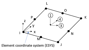
I, J, K, L, M, N, O, P (J - P are not required for all segment types)
- Degrees of Freedom
UX, UY, UZ, TEMP, VOLT, MAG, PRES, TTOP, TBOT (determined by the associated 3D contact elements: CONTA174, CONTA175, or CONTA177)
ROTX, ROTY, ROTZ are also valid, but only for the pilot node associated with a surface-based constraint or a rigid target surface
- Real Constants
R1, R2, (the others are defined through the associated CONTA174, CONTA175, or CONTA177 elements)
- Material Properties
None
- Surface Loads
Pressure, Face 1 (I-J-K-L) (opposite to target normal direction); used for fluid pressure penetration loading. On the SFE command use
LKEY= 1 to specify the normal pressure values andLKEY= 2 to specify starting and penetrating points. UseLKEY= 3, 4 to specify the tangential pressure values along the x and y direction of the element coordinate system (ESYS).- Body Loads
None
- Special Features
Birth and death Fluid pressure penetration Linear perturbation Nonlinear adaptivity Nonlinearity Rezoning Section definition for geometry correction of spherical and revolute surfaces - KEYOPT(1)
Element order (used by AMESH and LMESH commands only):
- 0 --
Low order elements
- 1 --
High order elements
- KEYOPT(2)
Boundary conditions for rigid target nodes:
- 0 --
Automatically constrained by the program. This option is valid only for static and full transient analyses. You should apply constraints manually for downstream analyses.
- 1 --
Specified by user
- KEYOPT(3)
Behavior of thermal contact surface:
- 0 --
Based on contact status
- 1 --
Treated as a free-surface regardless of the contact status
- 2 --
Treated as an insulated thermal condition (no convection/radiation to the environment) when the contact status is far-field. Near-field convection/radiation are considered.
- KEYOPT(4)
DOF set to be constrained on the dependent or independent DOF for internally-generated multipoint constraints (MPCs). This option is used for these situations: solid-solid and shell-shell assemblies; surface-based constraints that use a single pilot node for the target element; and rigid target surfaces that use the KEYOPT(2) = 1 setting.
- n --
Enter a six digit value that represents the DOF set to be constrained. The first to sixth digits represent ROTZ, ROTY, ROTX, UZ, UY, UX, respectively. The number 1 (one) indicates the DOF is active, and the number 0 (zero) indicates the DOF is not active. For example, 100011 means that UX, UY, and ROTZ will be used in the multipoint constraint. Leading zeros may be omitted; for example, you can enter 11 to indicate that UX and UY are the only active DOF. If KEYOPT(4) = 0 (which is the default) or 111111, all DOF are constrained.
Note: KEYOPT(4) is not supported for target elements used in a general contact definition.
- KEYOPT(5)
DOF set to be used in internally-generated multipoint constraints (MPCs) with the MPC algorithm and no separation or bonded behavior (KEYOPT(2) = 2 and KEYOPT(12) = 4, 5, or 6 on the contact element). Note that this key option is not used for surface-based constraints. (See Controlling Degrees of Freedom Used in the MPC Constraint in the Contact Technology Guide for more information):
- 0 --
Automatic constraint type detection. The default option internally sets KEYOPT(5) to the appropriate value for each contact constraint:
For a solid-solid assembly, the program sets KEYOPT(5) = 1 if the initial gap/penetration is smaller than 0.001*pinball; otherwise it sets KEYOPT(5) = 4.
For a shell-shell assembly, the program sets KEYOPT(5) = 2 if the initial gap/penetration is smaller than 0.001*pinball; otherwise it sets KEYOPT(5) = 4.
For a shell-solid assembly, the program always sets KEYOPT(5) = 4.
For a beam-to-solid or beam-to-shell assembly, it sets KEYOPT(5) = 5.
The default option also sets KEYOPT(5) internally to the appropriate value for the entire contact pair.
For potential over-constrained pairs, it sets KEYOPT(5) = 4.
For non-smooth bonding interfaces, it sets KEYOPT(5) = 4.
- 1 --
Projected constraint if an intersection is found from the contact normal to the target surface. Only translational DOFs are included in the constraint set.
- 2 --
Projected constraint if an intersection is found from the contact normal to the target surface. Both translational DOFs and rotational DOFs are included in the constraint set in an uncoupled manner.
Also used with a penalty-based shell-shell assembly (KEYOPT(2) = 0 or 1 and KEYOPT(12) = 5 or 6 on the contact element); see Bonded Contact for Shell-Shell Assemblies in the Contact Technology Guide for more information.
- 3 --
Force-distributed constraint - normal projection only. Both translational DOFs and rotational DOFs are included in the constraint set in a coupled manner if an intersection is found from the contact normal to the target surface. (Only translational DOFs from the target surface are included in the constraint set.)
- 4 --
Force-distributed constraint - all directions. This option acts the same as KEYOPT(5) = 3 if an intersection is found from the contact normal to the target surface. Otherwise, constraint equations are still built as long as contact nodes and target segments are inside the pinball region.
- 5 --
Force-distributed constraint - anywhere inside the pinball region. Constraint equations are always built as long as contact nodes and target segments are inside the pinball region, regardless of whether an intersection exists between the contact normal and the target surface.
- 6 --
Rigid surface constraint - normal projection only. If an intersection is found from the contact normal to the target surface, both translational DOFs and rotational DOFs are included in the constraint set in a coupled manner.
- 7 --
Rigid surface constraint - anywhere inside the pinball region. If an intersection is not found from the contact normal to the target surface, the rigid surface constraint equations are built as long as contact nodes and target segments are inside the pinball region. If an intersection is found from the contact normal to the target surface, this option acts the same as KEYOPT(5) = 6.
Note: When the no separation option (KEYOPT(12) = 4 on the contact element) is used with the MPC approach, only the KEYOPT(5) = 0 and 1 options (auto detection or projected constraint with translational DOFs only) described above are valid.
Note: KEYOPT(5) is not supported for target elements used in a general contact definition.
- KEYOPT(6)
Symmetry condition of a constrained surface defined by a force-distributed constraint or a rigid surface constraint, which uses a single pilot node for the target element.
The following KEYOPT(6) setting applies only to a force-distributed constraint defined on the symmetry surface of a typical symmetric model:
n--Enter a three digit value that represents the symmetry conditions on the constrained surface. Symmetry is defined with respect to the nodal coordinate system of the pilot node. The first, second, and third digits represent a symmetry condition with respect to the xy, xz, and yz planes, respectively. The number 1 (one) indicates a symmetry condition, and the number 0 (zero) indicates no symmetry condition. For example, KEYOPT(6) = 110 means the force distributed constraint is built on a surface or edge that has symmetry about the xy and xz planes. Leading zeros may be omitted (for example, KEYOPT(6) = 10 indicates symmetry about the xz plane only).
The following KEYOPT(6) setting applies only to a force-distributed constraint or a rigid surface constraint defined in a cyclic symmetry or multistage cyclic symmetry model:
- 2 --
The force-distributed or rigid surface constraint is applied on a cyclic symmetry surface or a multistage cyclic symmetry surface. The pilot node must be rotated (NROTAT) into the cyclic coordinate system. For more information, see Loading Considerations in the Cyclic Symmetry Analysis Guide.
- 3 --
Impose axisymmetric conditions for 2D/2.5D to 3D assembly. See Modeling a 2D/2.5D-3D Solid Assembly for more detail.
Note: Keep the following points in mind when using this symmetry condition:
When a symmetry condition is used, the pilot node must be defined on the symmetry plane/edge.
KEYOPT(6) = 111 is not valid input.
Note: KEYOPT(6) is not supported for target elements used in a general contact definition.
- KEYOPT(7)
Standard KEYOPT(7) Usage
Weighting factor control key. This option is only used for a force-distributed constraint that uses a single pilot node for the target element.
- 0 --
Weighting factors are calculated internally based on the contact area of each contact node.
- 1 --
The weighting factor for each contact node is 1.
- 2 --
A user-defined weighting factor is used based on tabular input specified as real constant FKN.
Alternate KEYOPT(7) Usage with Rigid Target Constraints
Use KEYOPT(7) to define a tied or pin node as follows.
- 0 --
Defines a tied node for rigid target. This keyoption is valid when the designated node is defined by point segment type using TSHAP,
POINT. Note that the tied node definition will override target KEYOPT(4) only on the tied nodes.- 1 --
Defines a pin node for rigid target. This keyoption is valid when the designated node is defined by point segment type using TSHAP,
POINT. Note that pin node definition will override target KEYOPT(4) only on the pin nodes.
- KEYOPT(8)
Single- or double- sided target key. A KEYOPT(8) value greater than zero is only valid for a target surface overlayed on shells or rigid target surfaces.
- 0 --
Only allow single-sided target surface in contact.
- 1 --
Allow double-sided target surface in contact. Select the side based on the smallest distance of either gaps or penetrations for each contact constraint.
Note: KEYOPT(8)=1 only supports CONTA174 and CONTA175 for certain detection methods. See Double-Sided Target Surfaces for details.
- KEYOPT(9)
Beam-to-beam contact type. This option is only used for modeling beam-to-beam contact with the CONTA177 element:
- 0 --
External beam-to-beam contact
- 1 --
Internal beam-to-beam contact
Note: KEYOPT(9) is not supported for target elements used in a general contact definition.
- KEYOPT(10)
Standard KEYOPT(10) Usage
Stress stiffening effects for a force-distributed constraint or a rigid surface constraint defined using the MPC approach (KEYOPT(2) = 2):
- 0 --
Do not include stress stiffening.
- 1 --
Include stress stiffening.
Alternate KEYOPT(10) Usage with Fluid Penetration Loading
Fluid pressure applied to target elements.
- 0 --
No fluid pressure is applied on target elements. (default)
- 1 --
Fluid pressure is applied on target elements.
- KEYOPT(11)
Relaxation method applied to force-distributed constraints and rigid surface constraints defined using the MPC approach (KEYOPT(2) = 2 on the contact element), and to rigid bodies:
- 0 --
Do not use relaxation method.
- 1 --
Use relaxation method.
Note: When relaxation in enabled (KEYOPT(11) = 1), the following contact element real constants are used: FKN and FKT are translational and rotational relaxation coefficients, respectively; FTOLN and TNOP are translational and rotational relaxation tolerances, respectively.
Note: KEYOPT(11) is not supported for target elements used in a general contact definition.
- KEYOPT(12)
Thermal expansion effect applied to rigid surface constraints defined using the MPC approach or the Lagrange Multiplier method (KEYOPT(2) = 2 or 3 on the contact element), and to rigid bodies:
:
- 0 --
Do not include thermal expansion.
- 1 --
Include thermal expansion
Note: KEYOPT(12) is not supported for target elements used in a general contact definition.
TARGE170 Output Data
The solution output associated with the element is shown in Table 170.2: TARGE170 Element Output Definitions.
The Element Output Definitions table uses the following notation:
A colon (:) in the Name column indicates that the item can be accessed by the Component Name method (ETABLE, ESOL). The O column indicates the availability of the items in the file jobname.out. The R column indicates the availability of the items in the results file.
In either the O or R columns, “Y” indicates that the item is always available, a letter or number refers to a table footnote that describes when the item is conditionally available, and “-” indicates that the item is not available.
Table 170.2: TARGE170 Element Output Definitions
| Name | Definition | O | R |
|---|---|---|---|
| EL | Element Number | Y | Y |
| NODES | Nodes I, J, and K | Y | Y |
| ITRGET | Target surface number (assigned by the program) | Y | Y |
| TSHAP | Segment shape type | Y | Y |
| ISEG | Segment numbering | 1 | 1 |
| CONT:FPRS | Actual applied fluid penetration pressure (magnitude of normal and tangential) | Y | Y |
| FPRSN | Actual applied fluid penetration normal pressure | - | Y |
| FPTR, FPTS | Actual applied fluid penetration tangential pressure in R and S directions (x and y directions of ESYS) | - | Y |
You can display or list the actual fluid pressure applied to the target element through several POST1 postprocessing commands, as shown below:
PLESOL,CONT,FPRS
PLNSOL,CONT,FPRS
PRESOL,CONT
PRNSOL,CONT
Note that only the FPRS (fluid penetration pressure) output item is meaningful when the PRESOL and PRNSOL commands are used for target elements.
Table 170.3: TARGE170 Item and Sequence Numbers lists output available through the ETABLE command using the Sequence Number method. See Creating an Element Table in the Basic Analysis Guide and The Item and Sequence Number Table in this reference for more information. The following notation is used in Table 170.3: TARGE170 Item and Sequence Numbers:
- Name
output quantity as defined in the Table 170.2: TARGE170 Element Output Definitions
- Item
predetermined Item label for ETABLE command
- E
sequence number for single-valued or constant element data
- I,J,K,L
sequence number for data at nodes I, J, K, L
TARGE170 Assumptions and Restrictions
Generally speaking, you should not change real constants R1 or R2, either between load steps or during restart stages; otherwise the program assumes the radii of the primitive segments varies between the load steps. When using direct generation, the real constants for cylinders, cones, and spheres may be defined before the input of the element nodes. If multiple rigid primitives are defined, each having different radii, they must be defined by different target surfaces.
For each pilot node, the program automatically defines an internal node and an internal constraint equation. The rotational DOF of the pilot node is connected to the translational DOF of the internal node by the internal constraint equation. Ansys, Inc. recommends against using external constraint equations or coupling on pilot nodes; if you do, conflicts may occur, yielding incorrect results.
For rotation of a rigid body constrained only by a bonded, rigid-flexible contact pair with a pilot node, use the MPC algorithm or a surface-based constraint as described in Multipoint Constraints and Assemblies in the Contact Technology Guide. Penalty-based algorithms can create undesirable rotational energies in this situation.
When using deformable TARGE170 elements overlaid on SOLID285 elements, make sure that KEYOPT(1) = 0 (the default) if you plan to use CDWRITE/CDREAD commands to write out model data and later read it back in. Otherwise, the TARGE170 elements will not be generated correctly after the CDREAD operation.