Use Separating, Morphing, Adaptive and Remeshing Technology (SMART) to simulate crack initialization in engineering structures.
The SMART method for crack initiation works with the SMART method for crack-growth. All primary requirements for SMART crack-growth simulation are respected.
The following topics for the SMART crack-initiation method are available:
Also see Adaptive Crack-Initiation and -Propagation in the Technology Showcase: Example Problems.
A SMART crack-initiation simulation is assumed to be quasi-static. It can be applied to perform a static or fatigue crack-growth simulation.
The following topics for crack-initiation analysis are available:
For more information, see Example: SMART Crack-Initiation/-Growth Analysis.
Issue Mechanical APDL commands to specify when and where a crack is initialized during the simulation. You can also set up the crack location, shape, and size.
The program uses the maximum principal stress as the criterion for determining when a crack is introduced. The maximum principal stress values are calculated at every finite element node and are compared with critical values. The critical value is input as a material property (TB,CRKI):
TB,CRKI, |
TBDATA,1, |
where Par1 is the critical value. |
Example 3.1: Defining the Criterion for the Critical Value
This input defines a critical value of 3.6 associated with material ID 1:
TB,CRKI,1
TBDATA,1,3.6
After specifying the critical value, input the crack information and control data, and connect other datasets (ADPCI):
ADPCI,DEFINE, |
| where: |
CIID is an integer ID number for identifying
your crack-initiation input data. Use the ID to display, track, and access
the associated data record later. |
CompName is a node-component name. Given
that models can include complicated deformations and geometry shapes, a
specific region of interest within the model may need to be distinguished to
bypass inessential stress concentrations caused by inappropriate boundary
conditions or contact settings. The node component highlights the initiation
zone accurately and reduces simulation loads. |
MAT_ID connects the critical value (defined
via TB,CRKI) with crack-initiation data records. |
CRACKGEOM characterizes crack geometry
information. ELLIPSE (for ellipse-shaped crack initiation) is the only valid
value. |
When the initiation criterion is reached, the program detects the intersection between the ellipse and the material and modifies local meshes automatically to generate crack fronts and crack surfaces.
Use either of these methods to define the ellipse geometry for crack initiation:
Defining a unique ellipse as follows:
ADPCI,GEOM, |
ADPCI,GEOM, |
ADPCI,GEOM, |
| where CENTER defines the center of the ellipse, AXES defines two ellipse orientations, and ALEN defines the axis lengths. |
Example 3.2: Defining an Ellipse-Shaped Crack
This input defines an ellipse-shape crack, initialized in a zone described by the node component CrkInitZone:
ADPCI,DEFINE,1,CrkInitZone,1,ELLIPSE
ADPCI,GEOM,1,CENTER,0,10,20
ADPCI,GEOM,1,AXES,1,0,0,0,1,0
ADPCI,GEOM,1,ALEN,0.1,0.2
The ellipse center is located at the position (0,10,20). The first orientation of the ellipse is (1,0,0) and the second is (0,1,0). The length of the first axis is 0.1 and the length of the second is 0.2.
|
Alternate ADPCI,GEOM command for defining the ellipse center and axes: You can also set up the ellipse center and orientations as follows:
The local coordinate system origin locates the ellipse center, and the X and Z axes define the first and second orientations, respectively. The LCS argument is equivalent to combining ADPCI,GEOM,,CENTER and ADPCI,GEOM,,AXES. |
If you do not wish to specify crack-initiation geometry inputs, omit the ADPCI,GEOM command. Doing so allows Mechanical APDL to calculate all data necessary for characterizing the elliptical crack automatically.
At the end of each substep, the program flags all nodes that have satisfied the initiation criterion and groups them into a single node cloud. The geometric center of the node cloud is the center of the ellipse. The nearest node to the ellipse center is called the seed node.
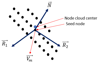
The program determines the two ellipse axes directions by:
Calculating the external normal direction
 at the seed node.
 The first axis
 of the ellipse is defined as the negative of
 :
:
so that the first axis points to the inside of the model.
Generating the covariance matrix based on all nodes in the node cloud, then calculating its three eigenvalues and eigenvectors.
The eigenvector associated with the largest eigenvalue is picked up. The cross product of vector
 and
and  defines the plane normal for the ellipse
 :
:
Calculating the cross product of vector
 and
and  as the second axis direction:
Vectors
 and
and  together define the ellipse orientations.
The program determines the axes lengths by:
Calculating
 by averaging element sizes around the seed
node.
by averaging element sizes around the seed
node.Assigning
 as the length of the first axis, and
 as the length of the second.
It is assumed that microdamage typically introduces a longer dimension along the exterior surface tangential direction rather than along the direction pointing into the model.
In cases where more than one eigenvector is associated with the largest
eigenvalue, remains unchanged, and the maximum principal stress
direction is set as  .
.  is generated via the same equation (
 ).
).
For embedded crack-initiations, where the crack-initiation zones cover volume materials instead of just model surfaces, Mechanical APDL sets the averaged maximum principal-stress direction as the normal direction of the crack plane. The major and minor ellipse axes are defined via projections of eigenvectors on the crack plane.
As one component of the Mechanical APDL fracture-analysis capability, the SMART crack-initiation method works with SMART crack-growth simulation.
After creating your crack-initiation model, define the parameters necessary for fracture-parameter calculation (CINT):
Create the fracture-parameter set:
CINT,NEW,SETNUMBERwhere
SETNUMBERis an integer value indicating the fracture-parameter set ID used to identify the fracture parameter for the crack-growth criterion.Calculate the fracture parameter:
CINT,TYPE,FractureParameterwhere
FractureParameteris JINT (J-integral) or SIFS (stress-intensity factors).Associate the crack-initiation data with crack-growth:
CINT,INIT,ADPCIIDwhere
ADPCIIDis the integer ID number that you specified (ADPCI,DEFINE) for identifying your crack-initiation input data.Specify the number of contours for fracture-parameter calculation:
CINT,NCON,NUMCONTOURSwhere NUMCONTOURS is the number of contours (default = 3) for fracture-parameter calculation.
Specify the nodal components for the nodes on the crack surfaces:
CINT,SURF,Par1,Par2where
Par1andPar2are the node-component names for the nodes on the two crack surfaces, respectively.Unlike a typical CINT,SURF definition, these two nodal components in a crack-initiation analysis remain empty. The program fills the node list automatically during crack initiation and local mesh changes.
If you do not explicitly issue node-component names for the crack surfaces, two internal node components are generated automatically. If you specify your own component names, however, you can display the components in the Mechanical APDL program's graphical tools (such as those available in the POST1 postprocessor).
For a crack-initiation analysis, CINT commands to describe crack fronts and surfaces (such as CINT,CTNC/CENC/NORM) are not used, as such data is unavailable until a crack is initialized.
Messages such as the followings are output to display criterion evaluation results:
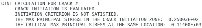
The maximum principal stress and the critical values are obtained at the location with the maximum ratio of (maximum principal stress) / (critical value), an important consideration in cases where critical values are not constant in the crack-initiation zone (such as those defined by tables or varying with temperatures). Therefore, the crack may be initiated at a location with a smaller absolute maximum principal stress value, but a larger (maximum principal stress) / (critical value) ratio.
Besides the usual prerequisites for the standard SMART crack-growth simulation, the following conditions apply in a crack-initiation analysis:
A SMART crack-initiation simulation requires and works with a SMART crack-growth simulation.
The ellipse size is not calculated if the ellipse axes are user-defined; therefore, issue ADPCI,ALEN if also issuing the command with the AXES or LCS argument.
The crack-initiation criterion is evaluated when CINT results are calculated at each substep; therefore, write solution-result data to the database at all substeps until a crack is initiated (OUTRES,CINT).
For embedded crack initiation, the crack initiation zones defined with node components are not preserved during remeshing, but a surface crack initiation zone is preserved prior to initiation in this specific area. For example, if a model contains both pre-existing cracks and newly initialized cracks, the remeshing for the pre-existing cracks may change the meshes associated with embedded crack initiation zones. This could lead to incorrect initiation predictions. One approach is to create a sufficient mesh between pre-existing cracks and initiation zones, which helps to avoid interference with initiation zone meshes prior to crack initiation.
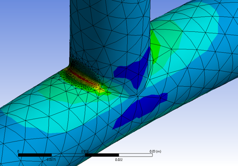
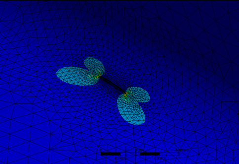
The following figures show an X-joint model and setup for a crack-initiation/-growth analysis:
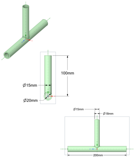
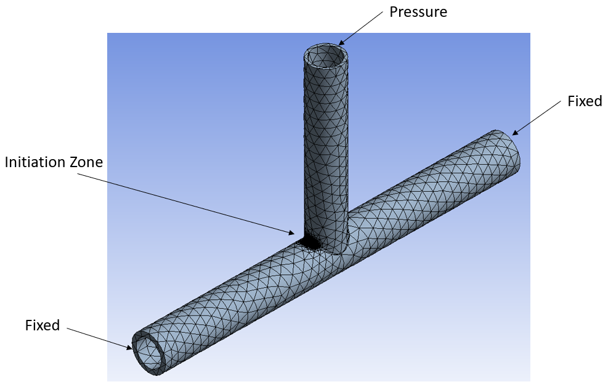
The left and right ends are fixed. A pressure load is applied on the top surface. To obtain accurate results, a finer mesh is used.
A relatively fine mesh is always recommended at the crack-initiation zone. A coarser mesh can be used for the remaining parts, reducing computational requirements and improving analysis speed.
| Material Properties and Loads | |||
|---|---|---|---|
| Young’s Modulus (Pa) | Poisson’s Ratio | Pressure (Pa) | Critical Maximum Principal Stress (Pa) |
| 2e11 | 0.3 | -100 | 145 |
This input defines a critical maximum principal stress value as the crack-initiation criterion:
! Define a critical maximum principal stress value as the crack-initiation criterion
TB,CRKI,2
TBDATA,1,145

! Create the crack-initiation-zone node component
ADPCI,DEFINE,1,CrkInitZone,2,ELLIPSE

...

! After obtaining the APDCI data,
!    define the SMART crack-growth calculation set

! Define parameters for fracture-parameter calculation
CINT,NEW,11
CINT,TYPE,SIFS
CINT,NCON,4
CINT,INIT,1
CINT,SURF,CRKSURF1,CRKSURF2

! Specify crack-growth analysis options
CGROW,NEW,31
CGROW,CID,11
CGROW,METHO,SMART,REME
CGROW,STOP,DAMX,0.3
CGROW,FCOP,KIC,1e-1
The connection part of the joint exhibits a serious stress concentration. As the load increases, a crack initiates at the root position and continues to grow.