


The XFEM-based crack-growth simulation technique can be used to simulate fatigue crack-growth in engineering structures. The method offers a convenient engineering approach for simulating cracks and fatigue crack propagation without resorting to modeling the cracks or remeshing the crack-tip regions as the crack propagates.
Following are characteristics of the XFEM-based approach to simulating fatigue crack-growth:
Uses singularity-based XFEM.
Based on Paris' Law.[2]
Supports 2D and 3D fatigue crack-growth simulation in linear elastic isotropic materials only.
Ignores large-deflection and finite-rotation effects, crack-tip plasticity effects, and crack-tip closure or compression effects.
The following topics for XFEM-based fatigue crack-growth are available:
For more information about XFEM, see XFEM-Based Crack Analysis and Crack-Growth Simulation.
Mechanical APDL analyzes crack-growth in structural components subject to repeated or cyclic loading using linear elastic fracture mechanics (LEFM) concepts.
The crack-growth rate (crack-growth per cycle) is defined as:[2]

where:
 = crack length = crack length |
 = number of cycles, = number of cycles,  (where (where  , ,  = stress-intensity factors at the maximum and minimum loads,
respectively) = stress-intensity factors at the maximum and minimum loads,
respectively) |
 = stress/load ratio = stress/load ratio 
|
The current implementation of fatigue crack-growth simulation in Mechanical APDL is restricted to region II in the following figure:

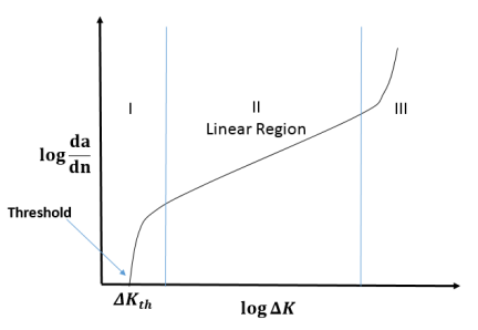
The variation in region II is typically described by Paris' Law:

where  and
and  are material constants that are determined experimentally.
(Several other relationships have been developed for regions I, II and III [3]).
are material constants that are determined experimentally.
(Several other relationships have been developed for regions I, II and III [3]).
For crack-growth involving mixed-mode fracture, the expression is modified as:

where the maximum circumferential stress criterion [4] is used to define

and


and  , the direction of crack propagation, is defined using the maximum
circumferential stress criterion:
, the direction of crack propagation, is defined using the maximum
circumferential stress criterion:

Only cyclic loadings of constant amplitudes are allowed, as shown:
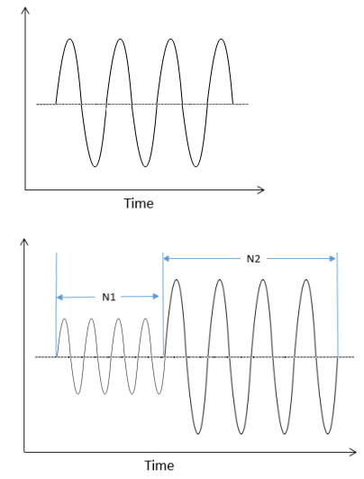
If the cyclical loading is such that the amplitude changes after some
 number of cycles, then each set of
  cycles with the same load amplitude should be modeled
separately as a load step. Overloading
can also be modeled in a similar manner.
cycles with the same load amplitude should be modeled
separately as a load step. Overloading
can also be modeled in a similar manner.
A typical fatigue crack-growth calculation requires:
Calculation of
 at the maximum load
Calculation of
 at the minimum load (or using the stress/load ratio
 )
)
Calculation of the crack increment

or
Calculation of the incremental number of cycles

Stopping the analysis if the specified maximum crack extension is reached
Mechanical APDL calculates or  (via the stress ratio) numerically during the analysis. The determination of
or depends on the fatigue crack-growth method. The program uses a
simple smoothing algorithm to smooth the calculated SIFS values for a given
crack front before calculating the or .
(via the stress ratio) numerically during the analysis. The determination of
or depends on the fatigue crack-growth method. The program uses a
simple smoothing algorithm to smooth the calculated SIFS values for a given
crack front before calculating the or .
The calculation of  or
or  (via the stress ratio
  ) is performed numerically during the analysis.
The determination of  or
or  depends on the fatigue crack-growth method.
A fatigue crack-growth can be modeled via either of these methods:
The LC method is typically used with constant-amplitude cyclic loads.
The maximum crack-extension increment  is user-specified, and the program calculates the number
of incremental cycles
is user-specified, and the program calculates the number
of incremental cycles  based on the fatigue crack-growth law.
|
LC Method Restrictions 2D XFEM-based fatigue crack-growth:
3D XFEM-based fatigue crack-growth: If multiple cracks exist in a model, the number of cycles may be estimated differently for different cracks in the same model.
|


The CBC method is suitable for variable-amplitude cyclic loadings and overload simulations.
The incremental cycles  are user-specified, and the crack-extension increment
 is calculated by the program based on the fatigue
crack-growth law.
is calculated by the program based on the fatigue
crack-growth law.
|
Restrictions 2D XFEM-based fatigue crack-growth:
3D XFEM-based fatigue crack-growth:
|


The analysis is assumed to be quasi-static and uses the singularity-based method.
Following is the general process for performing the analysis:
Defining an initial crack using the singularity-based XFEM approach. See Defining the Model in an XFEM Analysis.
For fatigue crack-growth analysis, the following considerations apply:
In a 2D XFEM analysis, the initial crack must cut the element(s) fully. For a 3D analysis, the crack can cut the elements partially or fully.
Only PLANE182 and SOLID185 elements (with the KEYOPT settings shown in Table 3.1: Elements Used in an XFEM Analysis) can be used.
Only linear elastic isotropic material behavior is supported.
Issue the following commands to invoke Paris' Law:
A fatigue crack-growth analysis uses the static analysis procedure only:
ANTYPE,STATIC
By default, the loading is assumed to be step-applied. (KBC,1 is enforced automatically.)
The total time specified (TIME) has no direct effect on the loading or the boundary conditions.
Each substep of the analysis load step yields a finite element solution during which the solution parameters are calculated and the crack is propagated. You can issue the DELTIM or NSUBST command to control the extent of crack propagation in a given load step.
A fatigue crack-growth analysis typically uses fixed time-stepping. Although you can use an automatic time-stepping scheme, it does not accelerate or decelerate the crack-propagation rate.
If using the LC method, the program controls the crack-growth increment during a substep. If using the CBC method, a value that you specify (CGROW,FCG,DN) controls the incremental number of cycles during a substep.
Evaluate the stress-intensity factors (SIFS), as follows:
Specify a new domain-integral calculation (where
IDis a number that you specify to identify this crack-calculation):CINT,NEW,
IDSpecify the desired fracture parameter:
CINT,TYPE,SIFS
Specify the element component name (
CompName) containing the crack-front element set:CINT,CFXE,
CompNameSpecify the number of contours (n) required:
CINT,NCON,
n
Mechanical APDL calculates  ,
,  and
and  by averaging the SIFS over contours 3 through
n.
The crack-growth calculations occurs in the solution phase after the solution has converged. Set the crack-growth calculation parameters as follows:
Initiate the crack-growth set (where
SETNUMis the crack-growth set number):CGROW,NEW,
SETNUMSpecify the crack-calculation ID (the same numerical identifier that you specified when setting up this fracture-parameter calculation (CINT,NEW,
ID)):CGROW,CID,
IDSpecify the XFEM crack-growth method:
CGROW,METHOD,XFEM
Specify the fatigue crack-growth law (where
MATIDis the material ID (TB,CGCR)):CGROW,FCOPTION,MTAB,
MATIDIf this command is not issued, the crack does not propagate.
Optional: Stop the analysis when the maximum crack extension is reached:
CGROW,STOP,CEMX,
Value
Perform the fatigue crack-growth calculation according the method chosen (LC or CBC):
3.9.2.6.1. Life-Cycle (LC) Method
Specify fatigue crack-growth using the LC method:
CGROW,FCG,METH,LC
Specify the maximum crack-growth increment:
CGROW,FCG,DAMX,
VALUEOptional: Specify the minimum crack-growth increment:
CGROW,FCG,DAMN,
VALUEOptional: Specify the minimum equivalent stress-intensity factor:
CGROW,FCG,DKTH,
VALUEThe crack does not propagate if the program-calculated
 is below
 VALUE.Specify the stress/load ratio:
CGROW,FCG,SRAT,
VALUE
3.9.2.6.2. Cycle-by-Cycle (CBC) Method
Specify fatigue crack-growth using the CBC method:
CGROW,FCG,METH,CBC
Optional: Specify the maximum (DAMX) and minimum (DAMN) allowable crack increments:
Specify the incremental number of cycles:
CGROW,FCG,DN,
VALUEOptional: Specify the minimum equivalent stress-intensity factor:
CGROW,FCG,DKTH,
VALUEThe crack does not propagate if the program-calculated
 is below
 VALUE.Specify the stress/load ratio:
CGROW,FCG,SRAT,
VALUE
2D and 3D analyses:
Fatigue crack-growth requires singularity-based XFEM.
Material behavior is assumed to be linear elastic isotropic.
Plasticity effects, nonlinear geometry effects, load-compression effects, and crack-tip-closure effects are not considered.
For cracks with short kinks, the SIFS may be only approximately path-independent (due to the limited number of contours that properly encompass the crack tip). This behavior may affect crack-direction prediction.
Restarting the analysis (ANTYPE,,RESTART) requires reissuing the CGROW command.
2D analysis only:
The maximum allowable crack increment is limited by the crack length in the element ahead of the tip. The minimum allowable crack increment must be smaller than the crack length in the element ahead of the tip; if it is larger, the crack increment is limited to the length of the crack in the element ahead of the tip.
Crack-path deviation can occur only at element edges (or faces). Crack propagation within an element occurs along a constant direction (determined when the element begins to crack).
Use the following standard POST1 (/POST1) commands for postprocessing fatigue crack-growth analysis results:
| Command | Purpose |
|---|---|
| ANDATA | Displays animated graphics data for nonlinear problems |
| ANTIME | Generates a sequential contour animation over a range of time |
| *GET | Retrieves a value and stores it as a scalar parameter or part of an array parameter |
| PLCKSURF | Plots the Φ = 0 level set surface in an XFEM-based crack analysis |
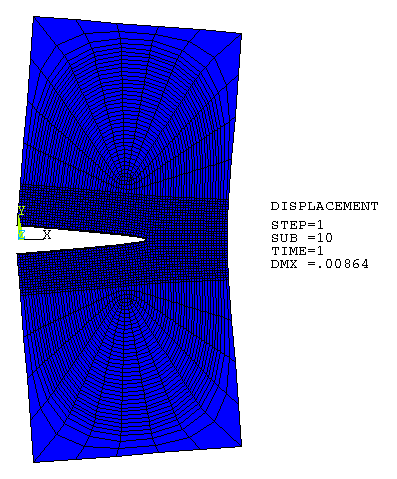
| PLDISP | Displays the displaced structure |
| PLESOL | Displays the solution results as discontinuous element contours |
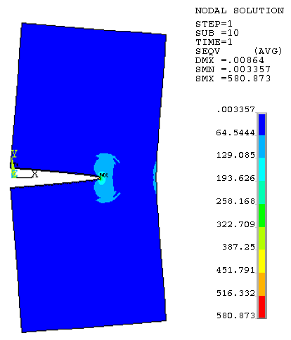
| PLNSOL | Displays results as continuous contours |
| PLVECT | Displays results as vectors |
| PRCINT | Prints fracture parameters and crack-growth information |
| PRESOL | Prints element solution results |
| PRNSOL | Prints nodal solution results |
| PRVECT | Prints results as vector magnitude and direction cosines |
To visualize the cracked elements in postprocessing, write the element miscellaneous data to the results file (OUTRES,MISC).
The POST26 time-history postprocessor (/POST26) is not supported.
This example analysis illustrates Mode I fatigue crack-growth simulation using the XFEM-based method. Fatigue crack-growth calculations apply Paris' Law. [2]
The problem uses a SEN specimen with a crack length (a) to width (W) ratio, a/W = 0.5:
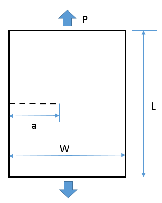
The specimen is subjected to a cyclical pressure P = 10.0 MPa with a stress/load
ratio  .
.
Table 3.6: Dimensions, Parameters and Constants
| Model Dimensions | W = 10.0 mm, L = 20.0 mm, a = 5 mm |
| Bulk Material Properties |

|
| Paris Law Constants |

|
The PLANE182 element (KEYOPT(1) = 0, KEYOPT(3) =0, KEYOPT(6) = 0) is used to model the specimen. A fine mesh is used in the region near the crack surface:
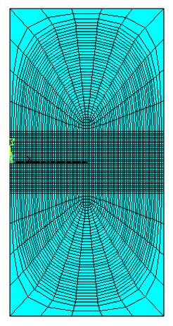
Linear elastic isotropic material behavior is assumed. The crack tip rests on the edge of the element.
Paris' Law is used to simulate fatigue crack-growth in the analysis. (See Table 3.6: Dimensions, Parameters and Constants for the Paris' Law constants.)
In the solution phase, fixed time-stepping is used. Each substep provides a linear elastic solution used to calculate the stress-intensity factors (SIFS) (CINT).
The theoretical value of the stress-intensity factor for the SEN specimen is given as: [5]

where:

and  is the applied pressure.
For fatigue crack-growth, the analysis uses the Life-Cycle (LC) method.
The CGROW command specifies the crack-growth-related
parameters. The command also specifies the fatigue crack-growth method and the
stress ratio  .
.
In the fatigue crack-growth LC method, the crack increment is fixed a priori (equal to the crack length in the element ahead of the current crack tip), and the incremental number of cycles is calculated for each substep.
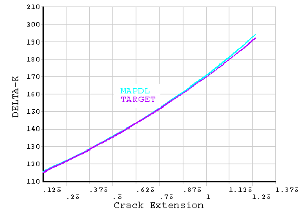
This figure shows the predicted number of cycles (MAPDL) versus the crack extension, as well as the theoretical results (TARGET):
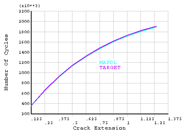
In this figure, too, the numerically calculated results (MAPDL) show good agreement with the theoretical results (TARGET):

Following is the input file used for the example fatigue crack-growth analysis of the SEN specimen:
/prep7

/com  Mode-I Fatigue Crack-Growth in a SEN specimen

! Model dimensions
a=5              !--- CRACK LENGTH
W=10             !--- WIDTH OF MODEL
H=20             !--- HEIGHT OF MODEL

! applied load
PRES=10

! Material model
E=2.0e5          !--- YOUNG MODULUS
NU=0.3           !--- POISSON'S RATIO
RO=1.0           !--- DENSITY

PI=ACOS(-1)

! Paris Law Constants
C=2.29E-13
M = 3

! Element types
et,1,182

! Continuum material behavior
mp, ex,   1, E
mp, nuxy,  1, NU
mp, dens, 1, R0

! Fatigue crack-growth Law Specification
tb, cgcr, 2, , , PARIS
tbdata, 1, C, M

! Define keypoints for base mesh
k, 1,  0.0, -2.0
k, 2,  W, -2.0
k, 3,  W, 2.0
k, 4,  0.0, 2.0

k, 5,  W,   -H/2
k, 6,  0.0, -H/2

k, 7,  0.0,  H/2
k, 8,  W,    H/2

! Define areas with KP
a, 1,2,3,4
a, 1,2,5,6
a, 3,4,7,8

! Set up the meshing size
xnume=79    ! number of elements in x,  which should be odd
ynume=33    ! number of elements in y , which should be odd
lsel,s,line,,1,3,2
LESIZE,all, , ,xnume, , , , ,1
lsel,s,line,,2,4,2
LESIZE,all, , ,ynume, , , , ,1


! Mesh the areas
type, 1
mat, 1
MSHKEY,1
amesh,1
esize,10/5
MSHKEY,0
amesh,2,3
allsel


! Element component required for XFENRICH command
esel, s, cent, y, -2,2
esel, r, cent, x,  0,9
cm, testcmp, elem
allsel

! mesh the crack surface with mesh200 elements
et, 2, 200, 0 ! keyopt(1) = 0 for mesh200 line elements

k, 9, 0.0, 0.0, 0.0
k, 10,10/79*40,0.0 , 0.0
l,9, 10! define a line

type, 2
mat, 2
lesize,11,,,12
lmesh,11
allsel

! element component for mesh200 elements
esel,s,type,, 2
cm, m200el, elem
allsel

! node component for crack front
nsel, s, loc,x,10/79*40
nsel,r,loc,y,0
nlist
cm, m200nd, node
allsel

! Define enrichment identification
xfenrich, ENRICH1, testcmp, , SING,1.5,0.01
allsel

! Define LSM values for cut elements
xfcrkmesh, ENRICH1, m200el, m200nd

/com
/com *************************************************************
/com
/com  		  INITIAL CRACK DATA
/com
/com *************************************************************
/com
xflist

! b.c. - bottom face
nsel, s, loc, y, -10.0
sf, all, pres, -PRES
allsel

! b.c. - top face
nsel, s, loc, y, 10.0
sf, all, pres, -PRES
allsel

! b.c - fix rbm - nodes on rt face
nsel, s, loc, x, 10.0
nsel, r, loc, y, -4/ynume/2*1.05,4/ynume/2*1.05
d, all, all, 0.
allsel
finish

! Solution Module
/solu
antype,0
time, 1.0
deltim, 0.1, 0.1,0.1
outres,all, all

!Fracture Parameter calculations
CINT, NEW, 1
CINT, CXFE,  _XFCRKFREL1
CINT, TYPE, SIFS, 2
CINT, NCON, 8
CINT, NORM, 0, 2


!CGROW calculations
cgrow, new, 1
cgrow, cid, 1
cgrow, method, xfem
cgrow, fcoption, mtab, 2

!Fatigue related data
CGROW, FCG, METH, LC  ! life-cycle method
CGROW, FCG, DAMX, 0.1 ! maximum crack-growth increment
CGROW, FCG, SRAT, 0 ! stress ratio

kbc, 1  ! loads are stepped for fatigue analysis

solve
finish

/post1
! get the # of data sets on the results file
*get, ndatasets, active, 0, set, nset

!define table if *VPLOT is used
*DIM,DN,array,ndatasets,2
*DIM,DA,array,ndatasets,2
*DIM,DK,array,ndatasets,2
*DIM,a_step,array,ndatasets,1

!loop on data sets and store results
set, , , , , , , 1 ! read the data set
*get, pval, CINT,1,CTIP,15910,CONTOUR,1,DTYPE,DLTN
 DN(1,1) = pval
*get, pval, CINT,1,CTIP,15910,CONTOUR,1,DTYPE,DLTA
 DA(1,1) = pval
*get, pval, CINT,1,CTIP,15910,CONTOUR,1,DTYPE,dltk
 DK(1,1) = pval

*do,i,2,ndatasets
 set, , , , , , , i ! read the data set
 *get, pval, CINT,1,CTIP,15910,CONTOUR,1,DTYPE,DLTN
 DN(i,1) = pval + DN(i-1,1)
 *get, pval, CINT,1,CTIP,15910,CONTOUR,1,DTYPE,DLTA
 DA(i,1) = pval + DA(i-1,1)
 *get, pval, CINT,1,CTIP,15910,CONTOUR,1,DTYPE,dltk
 DK(i,1) = pval
*enddo

!Evaluate the SIFS and DeltaK for the 1st set
 set, , , , , , , 1 ! read the data set
 *get, pval, CINT,1,CTIP,15910,CONTOUR,1,DTYPE,DLTA
 a0 = pval
 DA(1,2)=a0
 a_step(1)=a0
 Z=1.12-0.23*((10/79*40)/W)+10.55*((10/79*40)/W)**2
 ZZ=-21.72*((10/79*40)/W)**3+30.39*((10/79*40)/W)**4
 ZZZ=PRES*SQRT(PI*(10/79*40))
 DeltK= ZZZ*(ZZ+Z)
 DK(1,2) = DeltK
 DeltN = a0/(C*(DeltK**M))
 DN(1,2) = DeltN

!Evaluate the SIFS and DeltaK for the subsequent sets
*do,i,2,ndatasets
 SET,NEXT
 *get, pval, CINT,1,CTIP,15910,CONTOUR,1,DTYPE,DLTA
  a_step(i) = a_step(i-1) + pval
 DA(i,2) = a_step(i)
 pval = a_step(i)

 Z=1.12-0.23*((a_step(i-1)+10/79*40)/W)+10.55*((a_step(i-1)+10/79*40)/W)**2
 ZZ=-21.72*((a_step(i-1)+10/79*40)/W)**3+30.39*((a_step(i-1)+10/79*40)/W)**4
 ZZZ=PRES*SQRT(PI*(a_step(i-1)+10/79*40))
 DeltK= ZZZ*(ZZ+Z)
 DK(i,2) = DeltK
 Nst = (pval-a_step(i-1))/(C*(DeltK**M))
 DeltN = DEltN + Nst
 DN(i,2) = DeltN
*enddo

*DIM,LABEL,array,ndatasets,1
*DIM,DNTab,table,ndatasets,1
*DIM,DATab,table,ndatasets,1
*DIM,DKTab,table,ndatasets,1

*do,i,1,ndatasets
 LABEL(i)=i
 *VFILL,DNTab(i,1),DATA,DN(i,1)
 *VFILL,DATab(i,1),DATA,DA(i,1)
 *VFILL,DKTab(i,1),DATA,DK(i,1)
*enddo

!Plot results

!/show,PNG
/view,1,1,1,1
/dscale,,0
!/graphics,power


/AXLAB,X,Crack Extension
/AXLAB,Y,Number Of Cycles
/GCOL,1,MAPDL
/GCOL,2,TARGET
*VPLOT,DATab(1,1),DNTab(1,1),2

/AXLAB,X,Crack Extension
/AXLAB,Y, DELTA-K
/GCOL,1,MAPDL
/GCOL,2,TARGET
*VPLOT,DATab(1,1),DKTab(1,1),2

/COM, ----------------------SOLVER RESULTS COMPARISON------------------------
/COM,
/COM,                    DK
/COM,
/COM,Step |    A value    |   TARGET  |    Mechanical APDL
/COM,
/COM,  --------------------
/COM,
*VWRITE,LABEL(1),DA(1,1),DK(1,2),DK(1,1)
(F3.0,'   ',F14.8,'  ',F14.8,'   ',F14.8)

/COM, ----------------------SOLVER RESULTS COMPARISON------------------------
/COM,
/COM,                    DN
/COM,
/COM,Step |    A value    |   TARGET  |    Mechanical APDL
/COM,
/COM,  --------------------
/COM,
*VWRITE,LABEL(1),DA(1,1),DN(1,2),DN(1,1)
(F3.0,'   ',F14.8,'  ',F14.2,'   ',F14.2)

finish