


The following types of fracture-parameter calculations are available:
J-integral (CINT,TYPE,JINT)
Stress-intensity factors (CINT,TYPE,SIFS)
Material force (CINT,TYPE,MFOR)
C*-integral (CINT,TYPE,CSTAR)
VCCT energy-release rate (CINT,TYPE,VCCT)
Also see Unstructured-Mesh Method (UMM). The UMM a numerical tool for evaluating fracture-mechanics parameters more accurately in cases where unstructured hexahedral meshes and tetrahedral meshes are used.
The J-integral evaluation is based on the domain integral method by Shih[5]. The domain integration formulation applies area integration for 2D problems and volume integration for 3D problems. Area and volume integrals offer much better accuracy than contour integral and surface integrals, and are much easier to implement numerically. The method itself is also easy to use.
The following topics about J-integral calculation are available:
For a list of supported elements, see Table 2.1: Element Support for Fracture-Parameter Calculation. Also see Table 2.2: Material and Load Support for Fracture-Parameter Calculation.
For a 2D problem, the domain integral representation of the J-integral is given by:

where:
 = stress tensor = stress tensor |
 = displacement vector = displacement vector |
 = strain energy density = strain energy density |
 = Kronecker delta = Kronecker delta |
 = local coordinate axis = local coordinate axis |
 = crack-extension vector = crack-extension vector |
 = coefficient of thermal expansion = coefficient of thermal expansion |
 = initial strain tensor = initial strain tensor |
 = crack face traction = crack face traction |
 = integration domain = integration domain |
 = crack faces upon which tractions act = crack faces upon which tractions act |
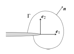
The direction of is the x axis of the local coordinate system ahead of the
crack tip. The q vector is chosen as zero at nodes along the contour Γ,
and is a unit vector for all nodes inside Γ except the midside nodes, if
there are any, that are directly connected to Γ. The program refers to
these nodes with a unit vector as virtual crack-extension
nodes.
For higher-order elements (such as PLANE183 and
SOLID186), the vector at midside nodes takes the averaged values from the
corresponding corner nodes.
For a 3D problem, domain integral representation of the J-integral becomes a volume integration, which again is evaluated over a group of elements.
Virtual crack-extension nodes are one of the most important input data elements required for J-integral evaluation. It is also referred to as the crack-tip node component.
For a 2D crack problem, the crack-tip node component usually contains one node which is also the crack-tip node. The first contour for the area integration of the J-integral is evaluated over the elements associated with the crack-tip node component. The second contour for the area integration of the J-integral is evaluated over the elements adjacent to the first contour of elements. This procedure is repeated for all contours. To ensure correct results, the elements for the contour integration should not reach the outer boundary of the model (with the exception of the crack surface).
For a 3D crack problem, the crack-tip node component consists of the nodes along the crack front. The crack-tip node component is not required to be sorted. The 3D J-integral contour follows a procedure similar to that of the 2D contour.
The program calculates the J-integral at the solution phase of the analysis after a substep has converged, then stores the value to the results file.
The CINT command initiates the J-integral calculation and specifies the parameters necessary for the calculation. See Fracture-Parameter Calculation Process.
The J-integral at the end nodes of a 3D open crack front is set to copy the J-integral at the adjacent nodes when using the unstructured mesh method (UMM) to calculate the fracture parameters.
Example 2.10: Using the CINT Command for J-integral Calculation
! J-integral calculation using crack-tip node component
!    and crack-plane normal
!
! local coordinate system
LOCAL,11,0,,,,
! select nodes located along the crack front and define
!   it as crack front/tip node component
NSEL,S,LOC,X,Xctip
NSEL,R,LOC,Y,Yctip
CM,CRACK_TIP_NODE_CM

! Define a new J-integral calculation
CINT,NEW,1
CINT, TYPE,JINT
CINT,CTNC,CRACK_TIP_NODE_CM
CINT,NORM,11,2
CINT,NCON,6
Mechanical APDL uses the interaction integral method to perform the stress-intensity factors (SIFS) calculation.
The following topics about SIFS calculation are available:
For a list of supported elements, see Table 2.1: Element Support for Fracture-Parameter Calculation. Also see Table 2.2: Material and Load Support for Fracture-Parameter Calculation.
The interaction integral is defined as:

where:
 = stress, strain and displacement (respectively) = stress, strain and displacement (respectively) |
 = stress, strain and displacement (respectively) of the
auxiliary field = stress, strain and displacement (respectively) of the
auxiliary field |
and  = crack-extension vector = crack-extension vector |
If thermal and initial strains exist in the structure and the surface tractions act on crack faces, the interaction integral is expressed as:

where:
 = thermal and initial strains (respectively) = thermal and initial strains (respectively) |
 = traction on crack surfaces = traction on crack surfaces |
For higher-order elements (such as PLANE183 and
SOLID186), the  vector, temperature values and initial strains at midside
nodes takes the averaged values from the corresponding corner nodes.
vector, temperature values and initial strains at midside
nodes takes the averaged values from the corresponding corner nodes.
The interaction integral is associated with the stress-intensity factors as

where:
 (i = 1,2,3) = Mode I, II, and III stress-intensity
factors (i = 1,2,3) = Mode I, II, and III stress-intensity
factors |
 (i = 1,2,3) = auxiliary Mode I, II and III
stress-intensity factors (i = 1,2,3) = auxiliary Mode I, II and III
stress-intensity factors |
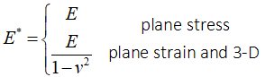
| E* = E for plane stress and E* = E / (1 - ν2) for plane strain |
| E = Young’s modulus |
| ν = Poisson’s ratio |
| μ = shear modulus |
The auxiliary crack-tip field specified in the equations in Understanding Interaction Integral Formulation is based on the local crack-tip coordinate systems. The auxiliary crack-tip fields are the asymptotic stress and strain fields for Mode I, Mode II, and Mode III crack configurations. [1]
To ensure the accuracy of the stress-intensity factors calculation, the local crack-tip coordinate system must have these characteristics:
The local x axis is pointed to the crack extension.
The local y axis is pointed to the normal of the crack surfaces or edges.
The local z-axis is pointed to the tangential direction of the crack front.
The local coordinate systems must be consistent across all nodes along the crack front. A set of inconsistent coordinate systems results in no path-dependency of the calculated stress-intensity factors and irregular behavior of the stress-intensity factor distribution along crack front. Mechanical APDL calculates the local coordinate systems based on the input crack front nodes and the normal of the crack surface or extension directions; however, because there may be insufficient information to determine a set of consistent coordinate systems, Ansys, Inc. recommends using either of these CINT command options:
For 2D crack models, the auxiliary field is selected according to the element type: axisymmetric, plane-stress, or plane-strain element.
For 3D crack models, Mechanical APDL determines whether a crack is closed or open. In a closed crack, the end-points of the crack front are the same (for example, a penny-shaped crack). In an open crack, the end-points of the crack front are distinct (for example, an edge crack in a compact-tension specimen).
For closed cracks, plane-strain auxiliary fields are used in the SIFS calculations.
For an open crack front, plane-stress auxiliary fields are used at the end nodes of the crack front, while plane-strain auxiliary fields are used at the interior nodes during the SIFS calculations.
For an open crack, you can control the behavior of auxiliary fields via
Par2 on the CINT command
(CINT,TYPE,SIFS,Par2
command):
Default: Plane-strain auxiliary fields on the interior nodes of the crack front (CINT,TYPE,SIFS or CINT,TYPE,SIFS,0). The stress-intensity factors at the end nodes are set to copy the stress-intensity factors at the adjacent nodes.
Plane-stress auxiliary fields over the entire open crack front (CINT,TYPE,SIFS,1).
Plane-strain auxiliary fields over the entire open crack front (CINT,TYPE,SIFS,2).
Selected auxiliary fields are valid for a single isotropic linear elastic material model in the crack-tip region. For the calculation of stress-intensity factors, Mechanical APDL does not support the use of more than one material model. If the material properties are temperature-dependent, the resulting material properties (such as Young’s modulus and Poisson’s ratio) must be constant in the entire region along the crack front.
For axisymmetric problems, results obtained using the interaction integral method may exhibit path-dependency. To mitigate the effects of path-dependency, use a fine mesh in the region near the crack tip.
Mechanical APDL calculates the stress-intensity factors using the interaction integral method at the solution phase of the analysis, and then stores the values to the results file.
Similar to the domain integral method for J-integral evaluation, the interaction integral method for stress-intensity factors calculation applies area integration for 2D problems and volume integration for 3D problems.
The CINT command initiates the stress-intensity factors calculations and specifies the parameters necessary for the calculation. See Fracture-Parameter Calculation Process.
Example 2.11: Using the CINT Command for Stress-Intensity Factors Calculation
! Stress-intensity factors calculation using the crack-tip
!   node component and the crack-plane normal
!
! local coordinate system
LOCAL,11,0,,,,
! select nodes located along the crack front and
!   define it as crack front/tip node component
NSEL,S,LOC,X,Xctip
NSEL,R,LOC,Y,Yctip
CM,CRACK_TIP_NODE_CM

! Define a new stress-intensity factors calculation
CINT,NEW,1
CINT,TYPE,SIFS
CINT,CTNC,CRACK_TIP_NODE_CM
CINT,NORM,11,2
CINT, NCON, 6
See VM256 for an example stress-intensity factors evaluation for a center crack in a plate.
The following topics about T-stress calculation are available:
For a list of supported elements, see Table 2.1: Element Support for Fracture-Parameter Calculation. Also see Table 2.2: Material and Load Support for Fracture-Parameter Calculation.
The T-stress parameter is calculated using an interaction integral similar to the one used for the stress-intensity factors calculation. The auxiliary solution used is the solution of a line load of magnitude f applied along the crack front in the direction of the crack plane:[12][13]

In practice, the magnitude of f is typically 1.
The T-stress itself is extracted from the interaction integral result I as follows:

where:
 = obtained T-stress value = obtained T-stress value |
|
 = Poisson’s ratio = Poisson’s ratio |
 = extensional strain at the crack front in the
direction tangential to the crack front = extensional strain at the crack front in the
direction tangential to the crack front |
T-stress evaluation supports the following material behavior:
Linear isotropic elasticity
T-stress evaluation does not support:
Pressure on cracks faces, body force, body temperature, and initial strains
Axisymmetric problems
The program calculates the T-stress at the solution phase of the analysis after a substep has converged, then stores the value to the results file.
The CINT command initiates the T-stress calculation and specifies the parameters necessary for the calculation. See Fracture-Parameter Calculation Process.
Example 2.12: Using the CINT Command for T-Stress Calculation
! T-stress calculation using the crack-tip node component,
!   the crack plane normal and the symmetry conditions
!
CINT,NEW,1
CINT,TYPE,TSTRESS
CINT,CTNC,CRACK_TIP_NODE_CM
CINT, NORM, 2
CINT,SYMM,ON
CINT,NCON,5
The material-force method determines the vectorial force-like quantities conjugated to the configurational change; that is, the method evaluates the material node point forces corresponding to the Eshelby stress and the material body forces.
When calculating material force for plastic problems, Ansys, Inc. recommends using the full model. Avoid using the symmetric model (CINT,SYMM,ON).
The following topics about material-force calculation are available:
For a list of supported elements, see Table 2.1: Element Support for Fracture-Parameter Calculation.
For a general 2D problem (in the absence of body forces, thermal strain and dynamic loads), the nodal material forces are defined as:

The Eshelby stress (Σ) is introduced in small-strain elasticity as:

In finite-strain elasticity, the Eshelby stress yields:

In the following figure, the directions of e1 and e2 correspond to the local coordinate system at the crack tip:
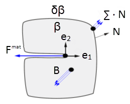
Here, e1 is the tangential component of the local coordinate system with respect to the crack surface, while e2 represents the normal component of the local coordinate system. The tangential component of the material-force vector Fmat, which is in the direction of e1, represents the scalar crack-driven force. In the numerical evaluation, the material force is calculated based on the resultant of all the material-force vectors in a user-defined domain β surrounding the crack tip.
If the plastic deformations exist in the structure, the material body forces acting on the domain are expressed as:

where B is the material body forces:

Here, Bp is the material body forces via plasticity, whereas Bt is the material body forces via thermal stress. Then, the material body forces via plasticity are expressed as:

If thermal strains exist in the structure, the nodal material body force vectors are:

For hyperelastic material, the material force is:

The Eshelby stress ( ) is defined as:

where  is the hyperelastic potential.
For a 3D problem, integral representation of the nodal material forces becomes a volume integration, which again is evaluated over a group of elements. The principal is similar to the 2D problem. After nodal material forces are evaluated, however, they are divided by a distance quantity through the thickness.
Virtual crack-extension nodes are critical input data elements required for material-force evaluation. The program uses virtual crack-extension node input to evaluate tangential (crack-driven force) and non-tangential components to the crack surface of the material-force vectors. The crack-extension nodes are typically grouped together as crack-tip node components.
For a 2D crack problem, the crack-tip node component typically contains one node, which is also the crack-tip node. The first contour for the area integration of the material force is evaluated over the elements associated with the crack-tip node component. The first contour gives nodal material force. The second contour for the area integration of the material-force approach is evaluated over the elements adjacent to the first contour of elements. The procedure is repeated for all contours. To ensure correct results, the elements for the contour integration should not reach the outer boundary of the model (with the exception of the crack surface).
For a 3D crack problem, the crack-tip node component consists of the nodes along the crack front. It is not necessary for the crack-tip node component to be sorted. The 3D material-force contour uses a procedure similar to that of the 2D contour.
The program calculates the material forces during the solution phase of the analysis after a substep has converged, then stores the values to the results file.
The CINT command initiates the material-force calculation and specifies the necessary parameters. See Fracture-Parameter Calculation Process.
Example 2.13: Using the CINT Command for Material-Force Calculation
! Material-force calculation using crack-tip node component, crack-plane normal,
!   and symmetry conditions
!
CINT,NEW,1
CINT,TYPE,MFOR
CINT,CTNC,CRACK_TIP_NODE_CM
CINT, NORM, 2
CINT,SYMM,ON
CINT,NCON,5
OUTRES,CINT,10     ! output material forces every 10 substeps
C*-integral is used to evaluate the crack tip fields in a homogenous material undergoing a secondary (steady-state) creeping deformation. C* is obtained by replacing the displacements with velocities, and the strain energy density with the strain energy rate density in the J-integral expansion.
To obtain path-independent C*-integral values, the creep deformation must be fully developed (that is, the creep strains should dominate the elastic strains in a region near the crack tip).
The following topics about C*-integral calculation are available:
For a list of supported elements, see Table 2.1: Element Support for Fracture-Parameter Calculation.
Also see C*-integral Evaluation for 3D Surface Flaws in the Technology Showcase: Example Problems.
For a 2D problem, and in the absence of thermal strain, body forces within the integration of area, and pressure on the crack surface, the domain integral representation of the C*-integral is given in C*-integral. For more information about the domain integral method, see J-integral Calculation.
The discretized form of the C*-integral is given by:

where  is the number of elements to be integrated,
  is the weight function, and
  is the area of the element represented by
  .
.
For higher-order elements (such as PLANE183 and
SOLID186), the  vector at midside nodes takes the averaged values from the
corresponding corner nodes.
vector at midside nodes takes the averaged values from the
corresponding corner nodes.
If the thermal strains exist in the structure and the surface tractions act on crack faces, the C*-integral is expressed as:

where  is the thermal expansion coefficient,
  is the crack face traction, and
  is crack face upon which the tractions act.
For a 3D problem, domain integral representation of the C*-integral becomes a volume integration, which again is evaluated over a group of elements. The implementation becomes more complicated; however, the principal is similar to that of the 2D problem.
C*-integral evaluation supports secondary (steady-state) creep material behavior. For more information, see Creep Option in the Material Reference.
Mechanical APDL calculates the C*-integral at the solution phase of the analysis after a substep has converged, then stores the value in the results file.
To start a C*-integral calculation, use the CINT command's NEW option and provide a numerical identifier for the input information for the calculation, as follows:
CINT,NEW,n
CINT,TYPE,CSTARwhere
nis the number identifying this C*-integral calculation.Example 2.14: Initiating a C*-integral Calculation
CINT,NEW,1       ! initiate a new C*-integral calculation
!                     as # 1
CINT,TYPE,CSTAR  ! set its type as CSTAR
All CINT command options available for J-integral calculation are available for C*-integral calculation.
Example 2.15: C*-integral Evaluation
Following is a C*-integral evaluation for a crack in a homogenous material with symmetry conditions imposed:
! local coordinate systems
local,11,0,,,,
! …

CINT,NEW,1
CINT,TYPE,CSTAR
CINT,CENC,CRACK_FRONT_NODE_SET,,11,2
CINT,SYMM,ON   ! crack 1 is a symmetrical crack
CINT,NCON,5
OUTRES,CINT,10  ! output C*-integral every 10 substeps
The approach for evaluating the energy-release rate is based on the virtual crack-closure technique (VCCT). The energy-release rate calculation occurs during the solution phase of the analysis and the results are saved for postprocessing.
The following topics about energy-release rate calculation are available:
For a list of supported elements, see Table 2.1: Element Support for Fracture-Parameter Calculation. Also see Table 2.2: Material and Load Support for Fracture-Parameter Calculation.
VCCT is based on the assumption that the energy needed to separate a surface is the same as the energy needed to close the same surface. The implementation described here uses the modified crack-closure method (a VCCT-based method) and assumes further that stress states around the crack tip do not change significantly when the crack grows by a small amount (Δa).
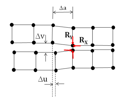
For 2D crack geometry with a low-order element mesh, the energy-release rate is defined as:


where:
| GI and GII = Mode I and II energy-release rate, respectively |
| Δu and Δv = relative displacement between the top and bottom nodes of the crack face in local coordinates x and y, respectively |
| Rx and Ry = reaction forces at the crack-tip node |
| Δa = crack extension, as shown in the following figure: |
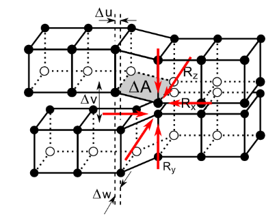
For 3D crack geometry with a low-order element mesh, the energy-release rate is defined as:


where:
| GI, GII, and GIII = Mode I, II, and III energy-release rate, respectively |
| Δu, Δv, and Δw= relative displacement between the top and bottom nodes of the crack face in local coordinates x, y, and z, respectively |
| Rx, Ry, and Rz = reaction forces at the crack-tip node |
| ΔA = crack-extension area, as shown in the following figure: |
In most cases, Ansys, Inc. recommends using linear elements including PLANE182 and SOLID185.
The accuracy of the VCCT calculation depends on the meshes. To ensure the greatest accuracy, use equal element sizes ahead of and behind the crack-tip node. The mesh size affects the solution; therefore, it is helpful to examine mesh-size convergence prior to attempting the finite element solution.
When calculating energy release rates (CINT,TYPE,VCCT), the mesh in the vicinity of the crack must contain only hex- (3D) or quad- (2D) shaped elements. The VCCT option does not support degenerative element shapes.
The VCCT method for energy-release rate calculation supports the following material behaviors:
Linear isotropic elasticity
Orthotropic elasticity
Anisotropic elasticity
The CINT command's VCCT option initiates the energy-release rate calculation and specifies the necessary parameters.
Following is the general process for calculating the energy-release rate:
Issue the CINT command twice, as shown:
CINT,NEW,n
CINT,TYPE,VCCT
where n is the identifier for this
energy-release rate calculation (for example, 1).
Similar to the J-integral calculation, the crack-tip node component and the crack-extension direction are both necessary for the energy-release rate calculation.
VCCT requires the finite element mesh to be in the crack-extension direction. To ensure the accuracy of the energy-release rate calculation, it is crucial that you correctly define the crack extension. How you do so depends upon whether the crack plane is flat or not:
This approach applies to both 2D crack geometry and 3D flat crack surfaces. It offers a simple way to define a 3D energy-release rate calculation, as you need only define the crack-tip (front) node component and the crack-plane normal.
|
2D Flat Crack Geometry For 2D crack geometry, define a crack-tip node component (usually a node located at the crack tip). You can also define a group of nodes around the crack tip, including the node at the crack tip. The program uses this group of nodes to form the necessary information for the VCCT calculation automatically. 3D Flat Crack Geometry For 3D flat crack surfaces, define a crack-tip node component that includes all of the nodes along the crack front. At each node location, however, only one node can exist. All nodes in the crack-tip node component must be connectable, and they must form a line based on the element connectivity associated with it. This line is the crack front. The program uses it to determine the elements and the nodes needed for the VCCT calculation automatically. VCCT is not applicable in the case of a collapsed crack-tip mesh. |
The command syntax is:
CINT,CTNC,Par1,Par2,Par3
where CTNC specifies a crack-tip node component,
Par1 is the crack-tip node component
name, Par2 is the crack-extension direction
calculation-assist node (any node on the open side of the crack), and
Par3 is the crack front’s end-node
crack-extension direction override.
The Par1 and
Par2 values help to identify the
crack-extension direction. Although the program automatically calculates
the energy-release rate at the crack tip using the local coordinate
system, it is usually best to use Par2 to
define a crack face node to help align the extension directions of the
crack-tip nodes.
By default, the program uses the external surface to determine the
crack-extension direction and normal when the crack-tip node hits the
free surface. You can use Par3 to override
this default.
After the crack-tip node component is defined, define the normal of the crack plane. The program automatically converts it into the crack-extension vector q, based on the element information. The crack-extension vector is taken along the perpendicular direction to the plane formed by the crack-plane normal and the tangent direction of the crack-tip node, and is normalized to a unit vector.
The command syntax is:
CINT,NORM,
Par1,Par2where
Par1is the coordinate system number andPar2is the coordinate system axis.
Example 2.16: Specifying Crack Information
!   Local coordinate system
LOCAL,11,0,,,,
! select nodes located along the crack front and
! define it as crack front/tip node component
NSEL,S,LOC,X,Xctip
NSEL,R,LOC,Y,Yctip
CM,CRACK_TIP_NODE_CM

!   Define a new the energy-release rate calculation
CINT,NEW,1
CINT,TYPE,VCCT
CINT,CTNC,CRACK_TIP_NODE_CM
CINT,NORM,11,2
Example 2.17: Specifying Crack Information
!   Select nodes located along the crack front and
!      define it as crack front/tip node component
LSEL,,,,
NSLL
CM,CRACK_FRONT_NODE_CM,NODE
CINT,NEW,1
CINT,TYPE,VCCT
CINT,CTNC,CRACK_FRONT_NODE_CM
This approach applies to 3D curved crack planes, where a unique normal may not exist. However, you must define the crack-extension node component and the crack-extension direction at each crack-tip node location:
Define a node component consisting of one or more nodes forming the crack tip.
The node component can have one or more nodes.
Example: CINT,CENC,
ComponentNameIf the node component has more than one node, identify the crack-tip node separately.
If a crack-tip node is not identified, the first node of the node component is used as the first node.
Example: CINT,CENC,
ComponentName,Node1Define the crack-extension direction.
Identify the local coordinate system associated with the crack under consideration, and identify the local axis along which the crack should extend.
Example: CINT,CENC,
ComponentName,Node1,11,2Alternatively, define the crack-extension direction by directly specifying the global X, Y, and Z components of the crack-extension vector.
Example: CINT,CENC,
ComponentName,Node1,,,compx,compy,compz
Repeat this method for all node locations along the crack front. Although the program automatically calculates the local coordinate system at the crack tip to determine the energy-release rate, it is usually best to use the NORM option to help align the calculated normals of the crack-tip nodes.
Example 2.18: Specifying Crack Information When the Crack Plane Is Not Flat
!   Local coordinate systems
local,11,0,,,,
local,12,0,,,,
! …
local,n,0,,,,

NSEL,S,LOC,X,Xctip1
NSEL,R,LOC,Y,Yctip1
NSEL,R,LOC,Z,Zctip1
CM,CRACK_FRONT_NODE_CM1
NSEL,S,LOC,X,Xctip2
NSEL,R,LOC,Y,Yctip2
NSEL,R,LOC,Z,Zctip2
CM,CRACK_FRONT_NODE_CM2
! …
NSEL,S,LOC,X,Xctipn
NSEL,R,LOC,Y,Yctipn
NSEL,R,LOC,Z,Zctipn
CM,CRACK_FRONT_NODE_CMn

CINT,NEW,1
CINT,TYPE,VCCT
CINT,CENC,CRACK_FRONT_NODE_CM1,,11,2
CINT,CENC,CRACK_FRONT_NODE_CM2,,12,2
! …
CINT,CENC,CRACK_FRONT_NODE_CMn,,n,2
Example 2.19: Specifying Crack Information When the Crack Plane Is Not Flat
!   Crack-extension node component and
!     crack-extension direction specification using vectors
NSEL,S,LOC,X,Xctip1
NSEL,R,LOC,Y,Yctip1
NSEL,R,LOC,Z,Zctip1
CM,CRACK_FRONT_NODE_CM1
NSEL,S,LOC,X,Xctip2
NSEL,R,LOC,Y,Yctip2
NSEL,R,LOC,Z,Zctip2
CM,CRACK_FRONT_NODE_CM2
! …
NSEL,S,LOC,X,Xctipn
NSEL,R,LOC,Y,Yctipn
NSEL,R,LOC,Z,Zctipn
CM,CRACK_FRONT_NODE_CMn

CINT,NEW,1
CINT,TYPE,VCCT
CINT,CENC,CRACK_FRONT_NODE_CM1,,,,Vx1,Vy1,Vz1
CINT,CENC,CRACK_FRONT_NODE_CM2,,,,Vx2,Vy2,Vz2
! …
CINT,CENC,CRACK_FRONT_NODE_CMn,,,,Vxn,Vyn,Vzn
Local Crack-Tip Coordinate System
The VCCT calculation is based on the local crack-tip coordinate systems. To ensure the accuracy of the energy-release rate calculation, it is crucial to have a local crack-tip coordinate system in which the local x axis is pointed to the crack extension, the local y axis is pointed to the normal of the crack surfaces or edges, and the local z-axis pointed to the tangential direction of the crack front.
Local coordinate systems must be consistent across all nodes along the crack front. A set of inconsistent coordinate systems results in irregular behavior of the energy-release rate distribution along crack front.
The program automatically calculates the local coordinate systems based on the input crack front nodes and the normal of the crack surface or extension directions. Because there may be not enough information to determine a set of consistent coordinate systems, however, Ansys, Inc. recommends:
If the crack is located along a symmetry plane, and only a half model is created, define a symmetric condition so that the program can account for it. To do so, issue the following command:
CINT,SYMM,ON
Example 2.20: Defining a Crack Symmetry Condition
CINT,NEW,1
CINT,TYPE,VCCT
CINT,SYMM,ON   ! crack 1 is a symmetrical crack
Similar to the J-integral calculation, the program calculates the energy-release rate during the solution phase of the analysis and stores the results in the .rst file for postprocessing.
Energy-release rate output uses all OUTRES defaults. OUTRES,ALL includes CINT command results. You can, however, issue OUTRES,CINT to control the specific output for energy-release rate results.
Example 2.21: Specifying Output Controls
CINT,NEW,1
CINT,TYPE,VCCT
CINT,CTNCP,CRACK_TIP_NODE_CM
CINT,SYMM,ON
OUTRES,CINT,10   ! output CINT results every 10 substeps