


Structural design concepts traditionally use a strength-of-material approach for designing a component. This approach does not anticipate the elevated stress levels due to the existence of cracks. The presence of such stresses can lead to catastrophic failure of the structure.
Fracture mechanics accounts for the cracks or flaws in a structure. The fracture-mechanics approach to the design of structures includes flaw size as one important variable, and fracture toughness replaces strength of material as a relevant material parameter.
Fracture analysis is typically accomplished using either the energy criterion or the stress-intensity-factor criterion. For the energy criterion, the energy required for a unit extension of the crack (the energy-release rate) characterizes the fracture toughness. For the stress-intensity-factor criterion, the critical value of the amplitude of the stress and deformation fields characterizes the fracture toughness. Under some circumstances, the two criteria are equivalent.
The following additional topics concerning fracture are available:
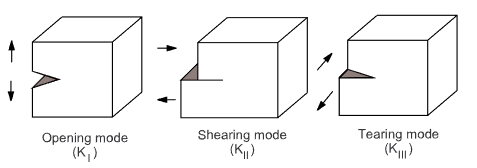
Depending on the failure kinematics (that is, the relative movement of the two surfaces of the crack), three fracture modes are distinguishable, as shown in Figure 1.1: Schematic of the Fracture Modes:
Mode I – Opening or tensile mode
Mode II – Shearing or sliding mode
Mode III – Tearing or out-of-plane mode
Fracture is generally characterized by a combination of fracture modes.
Typical fracture-mechanics parameters describe either the energy-release rate or the amplitude of the stress and deformation fields ahead of the crack tip.
The following parameters are widely used in fracture-mechanics analysis:
For more information, see:
J-integral is one of the most widely accepted fracture-mechanics parameters for linear elastic and nonlinear elastic-plastic materials. The J-integral is defined as:[2]:

where W is the strain energy density, T is the kinetic-energy density, σ represents the stresses, u is the displacement vector, and Γ is the contour over which the integration occurs. Mechanical APDL assumes T to be negligible and does not account for it in the calculations.
For a crack in a linear elastic material, the J-integral represents the energy-release rate. Also, the amplitudes of the crack-tip stress and deformation fields are characterized by the J-integral for a crack in a nonlinear elastic material.
For more information, see J-integral Calculation and J-integral as a Stress-Intensity Factor.
Hutchinson [3] and Rice and Rosengren [4] independently showed that the J-integral characterizes the crack-tip field in a nonlinear elastic material. They both assumed a power law relationship between plastic strain and stress. If elastic strain is included, the relationship for uniaxial deformation is given as:

where σ0 is the reference stress (the yield stress of the material), and ε0 = σ0/E, α is a dimensionless constant, and n is the hardening component. They showed that, at a distance very close to the crack tip and well within the plastic zone, the crack-tip stress and strain ahead of crack tip can be expressed as:

and

For elastic material, n = 1 and the above equation predicts the
 singularity which is consistent with linear elastic
fracture mechanics.
singularity which is consistent with linear elastic
fracture mechanics.
The energy-release rate, limited to linear elastic fracture mechanics, is based on the energy criterion for fracture proposed by Griffith and further development by Irwin. In this approach, the crack-growth occurs when the energy available for crack-growth is sufficient to overcome the resistance of the material.[1]
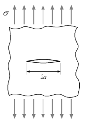
The energy-release rate G is defined in elastic materials as the rate of
change of potential energy released from a structure when a crack opens. For
example, the following illustration shows a crack of length
2a in a large elastic body with modulus E subject
to a tensile stress (σ):
The energy-release rate is given by:

At the moment of fracture, G is equal to the critical energy-release rate Gc, a function of the fracture toughness. The value of Gc for a material can be determined via a relatively straightforward set of crack experiments.
For a single-fracture mode, the stress-intensity factor and the energy-release rate are related by:

where G is the energy-release rate,  for plane strain, and
  for plane stress. (E is the material Young’s modulus,
and ν is the Poisson’s ratio.)
for plane stress. (E is the material Young’s modulus,
and ν is the Poisson’s ratio.)
For more information, see VCCT Energy-Release Rate Calculation.
Limited to linear elastic material, the stress and strain fields ahead of the crack tip are expressed as:


where K is the stress-intensity factor, r and θ are coordinates of a polar coordinate system (as shown in Figure 1.2: Schematic of a Crack Tip). These equations apply to any of the three fracture modes.

For a Mode I crack, the stress field is given as:


For more information, see Stress-Intensity Factors (SIFS) Calculation.
The asymptotic expansion of the stress field in the vicinity of the crack tip, expressed in the local polar coordinate system described in Figure 1.2: Schematic of a Crack Tip, is represented as:

where the first singular terms of this eigen-expansion (the terms involving
 ) are the stress-intensity factors, and the first non-singular
term (T) is the elastic T-stress.
) are the stress-intensity factors, and the first non-singular
term (T) is the elastic T-stress.
T-stress is the stress acting parallel to the crack faces. It is tightly linked to the level of crack-tip stress triaxiality; therefore, its sign and magnitude can substantially change the size and shape of the crack-tip plastic zone [14]. Negative T-stress values decrease the level of crack-tip triaxiality (leading to larger plastic zones), while positive values increase the level of triaxiality (leading to smaller plastic zones). A higher crack-tip triaxiality promotes fracture because the input of external work is dissipated less by the global plastic deformation and is therefore available to augment local material degradation and damage [15].
T-stress also plays an important role in the stability of straight crack paths submitted to Mode I loading conditions. For a small amount of crack-growth, cracks with T < 0 have been shown to be stable, whereas cracks with T > 0 tend to deviate from their initial propagation plane [16].
For more information, see T-stress Calculation.
Used primarily to analyze material defects such as dislocations, voids, interfaces and cracks, material force (also known as configurational force) can be understood by considering the presence of an inclusion in an elastic solid (matrix material), as shown in this figure:
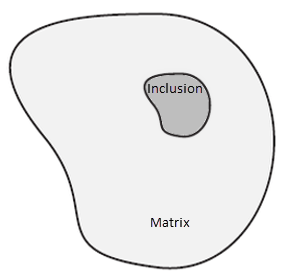
The force exerted by the matrix on the inclusion is the material force. When an inclusion is incorporated into a stress-free elastic body, the entire body undergoes a deformation, resulting in a configurational change of the body (or matrix) from its original state. The change in the total energy due to the deformation is characterized by the material force. The material force is typically calculated by evaluating the energy-momentum tensor (or Eshelby [17] stress tensor).
When the inclusion undergoes a uniform deformation, both the matrix and the inclusion experience an elastic stress field. Now, consider the following figure:
Figure 1.4: Thought Experiment Proposed by Eshelby
|
A. |
Isolate the inclusion from the matrix: 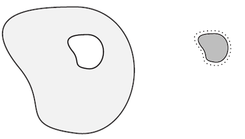 | No forces are applied to the inclusion or to the matrix. Because the inclusion is now isolated, it undergoes a homogenous deformation. The strains experienced by the inclusion are called eigenstrains. The matrix remains stress- and strain-free. |
|
B. |
Recover the original shape of inclusion by applying surface forces on the inclusion: 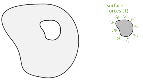 | The elastic strains induced in the inclusion due to applied surface traction cancel out the eigenstrains. The surrounding body remains stress- and strain-free. |
|
C. |
Replace the inclusion along with the applied surface forces: 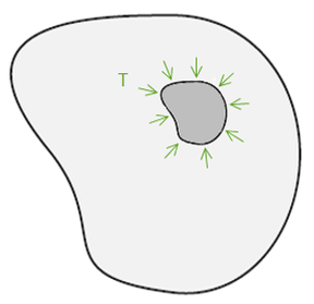 | No change of deformation occurs in either the inclusion or the matrix. |
|
D. |
Remove the applied surface forces: 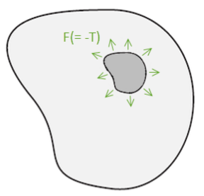 | By removing the surface forces, we return to the original problem of a body with an inclusion, as shown in Figure 1.3: Matrix with Inclusion. |
The change from step C to step D is that a body force (or surface force on the hole in the matrix where the inclusion is inserted), equal and opposite to the surface forces in step B, is applied.
The body (or surface) force is the material force. Essentially, the presence of an inclusion creates a variation in the strain energy density in the matrix material, leading to the material force acting on the inclusion and being allowed to move through the material.
The material force method essentially determines a vectorial force-like quantity conjugate to the eigenstrain. As a general description, the material force approach is defined for elasticity as described in Understanding the Material-Force Approach. [18]
For a crack in a linear or nonlinear elastic material, the tangential component of the material force vector to the crack surface represents the energy-release rate. Also, the crack propagation direction and inhomogeneity, flaws, and mismatched mesh can be characterized by the material force vectors. In plasticity, the tangential component of the material force vector to the crack surface represents the crack-driving force. [19]
For more information, see Material-Force Calculation.
As J-integral does for isotropic elastic materials, C*-integral characterizes the crack tip conditions in homogenous materials undergoing a secondary (steady-state) creeping deformation [20][21]. The C*-integral is defined as follows:

where  is the stress tensor,
  is the displacement rate vector,
  is the strain energy rate density,
  is the Kronecker delta,
  is the coordinate axis, and
  is the crack-extension vector.
For more information, see C*-integral Calculation, and C*-integral Evaluation for 3D Surface Flaws in the Technology Showcase: Example Problems.
Fracture/crack-growth is a phenomenon in which two surfaces are separated from each other, or material is progressively damaged under external loading. The following methods are available for simulating such failure:
For more information, see Crack-Initiation and -Growth Simulation, Interface Delamination, and Fatigue Crack-Growth.
Separating, Morphing, Adaptive and Remeshing Technology (SMART) is a computationally efficient, remeshing-based method for crack-growth simulation. The method uses a combination of techniques to update mesh changes, local to the crack-front region only, to simulate both static and fatigue crack-growth. For more information, see SMART Method for Crack-Growth Simulation.
This method uses interface elements (INTERnnn) with
VCCT to
simulate the fracture by separating the interface elements between two materials
with one or more user-specified fracture criteria. This approach applies to
homogeneous material fracture as well as interfacial fracture in biomaterial
systems. It is most suitable for interface delamination of laminate composites
with good numerical stability. For more information, see VCCT-Based Crack-Growth Simulation.
This method uses interface (INTERnnn) or contact
(CONTAnnn) elements to allow the separation of
the surfaces and the cohesive material model to describe the separation behavior
of the surfaces. This approach applies to both the simulation of fracture in a
homogeneous material as well as interfacial delamination along the interface
between two materials. For more information, see Crack-Initiation and -Growth Simulation, Interface Delamination, and Fatigue
Crack-Growth.
Gurson's model is a plasticity model (TB,GURSON) used to simulate ductile metal damage. The model is a micromechanics-based ductile damage model incorporating the void volume fraction into plasticity constitutive equation to represent the ductile damage process of void grow, void nucleation, and void coalescence. For more information, see Gurson's Model in the Mechanical APDL Theory Reference and the TB,GURSON command documentation.
The eXtended Finite Element Method (XFEM) is based on enriching the degrees of freedom in the model with additional displacement functions that account for the jump in displacements across the crack surface. The method is used to propagate cracks in linear elastic materials based on user-specified fracture criteria. For more information, see XFEM-Based Crack Analysis and Crack-Growth Simulation.