


A cyclic-loading analysis repeats a predefined loading cycle (or cycles) a specified number of times.
Each cyclic-loading solution–also referred to as a cyclic-loading load step–is comprised of several cycles associated with a single SOLVE command. The solution occurs in a single load step with multiple substeps.
An analysis can have multiple cyclic-loading solutions combined with noncyclic-loading solutions.
The following topics are available for cyclic-loading analysis:
This command initiates and sets solution parameters for a standard cyclic-loading analysis:
CLOAD, Option,
Input1 |
To specify the various control options (Option), issue
the command multiple times.
The following steps are involved in a standard cyclic-loading analysis:
- 6.1.1.1. Step 1: Define the Tabular Array
- 6.1.1.2. Step 2: Specify the Cyclic-Loading Table Values
- 6.1.1.3. Step 3. Apply the Cyclic-Loading Table(s)
- 6.1.1.4. Step 4. Specify Cyclic-Loading Parameters
- 6.1.1.5. Step 5. Specify Time-Stepping Parameters
- 6.1.1.6. Step 6. Select Output Time Points
- 6.1.1.7. Step 7. Solve the Cyclic-Loading Analysis
Define the tabular array (*DIM). Set the tabular array size according to the number of time points needed to define one cycle of loading.
You can define multiple tabular arrays defined to apply different loads in a cyclic-loading load step. (For example, one cyclic-loading table can apply a displacement boundary condition, another can apply a force loading, and so on.) If you intend to use multiple tabular arrays in the same cyclic-loading load step, the arrays must be of the same size. Different cyclic-loading load steps can have different array sizes.
Issue CLOAD,DEFINE,BEGIN and CLOAD,DEFINE,END commands before and after load table definitions, respectively, to mark tabular array or arrays as cyclic-loading tables.
Example 6.1: Marking Tabular Arrays as Cyclic-Loading Tables
CLOAD,DEFINE,BEGIN
*DIM,_cycload1,TABLE,4
*DIM,_cycload2,TABLE,4
CLOAD,DEFINE,END
Cyclic-loading tables to be applied in the same cyclic-loading load step must have the same dimensions.
Load tables not specified as cyclic-loading tables (CLOAD,DEFINE) as shown are not cyclically repeated.
Column 0 contains the time points of the cyclic-loading table, and column 1 contains the load values.
The cyclic-load table time value must always start at 0. The program sets the correct time value automatically when the current cyclic-loading analysis is preceded by a standard solution or another cyclic-loading analysis.
The beginning and ending load values must always be the same.
Example 6.2: Specifying Values in a Cyclic-Loading Table
! Time values
_cycload1(1,0) = 0.   ! time must start at 0
_cycload1(2,0) = 0.25
_cycload1(3,0) = 0.8
_cycload1(4,0) = 1.2
! Load values
_cycload1(1,1) = 0.   ! beginning load value
_cycload1(2,1) = 0.1
_cycload1(3,1) = -0.15
_cycload1(4,1) = 0.   ! ending load value
If there are multiple cyclic-loading tables in a given cyclic-loading load step, they must have the same time values.
Apply the cyclic-loading table(s) to the finite element problem.
Example 6.3: Applying Cyclic-Loading Tables
NSEL, S, LOC, Y, 10
D,All,UY,%_cycload1%
NSEL, S, LOC, X, 10
D,All,UX,%_cycload2%
Each cyclic-loading solution (comprised of multiple cycles) is its own load step. For each new cyclic-loading load step, you must reapply a cyclic-loading table or tables. Cyclic-loading load applications are not automatically carried from one cyclic-loading load step to another. It is not necessary to redefine the load tables (that is, steps 1 and 2 need not be repeated) if they already exist, or if they were applied previously.
Define the cyclic-loading analysis parameters by specifying the length of each loading cycle (CLOAD,CYCTIME) and total number of cycles (CLOAD,CYCNUM). The final time point of the defined cyclic-loading tables must coincide with the value of the cycle length.
Example 6.4: Defining Cyclic-Loading Parameters
CLOAD,CYCNUM,100   ! total number of cycles
CLOAD,CYCTIME,1.2  !time length of each cycle
Each cyclic-loading load step requires a specified number of cycles (CLOAD,CYCNUM) and cycle time (CLOAD,CYCTIME).
In a cyclic-loading analysis, the time-stepping parameters (NSUBST or DELTIM) require no adjustment if the total number of cycles (CLOAD,CYCNUM) are changed.
By default, time-stepping (NSUBST or DELTIM) applies to a single cycle length (and not the total analysis time).
As shown in this figure, time-stepping on a
single-cycle-length basis means that the time-stepping applies to
 :
:
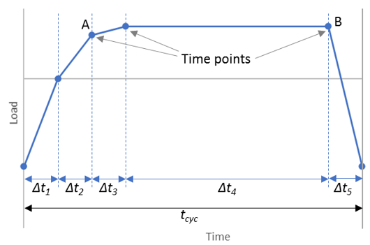
The program adjusts the time-stepping increments to ensure that the time points defined in the cyclic-loading table are not missed.
The program also disables the predictor at each defined table time point, as the defined table time point is often associated with a sudden change in loading direction, as shown:
When the load transition is smooth, the default time-stepping and predictor behavior may not be appropriate.
Consider a sinusoidal cyclic-loading of the form shown:
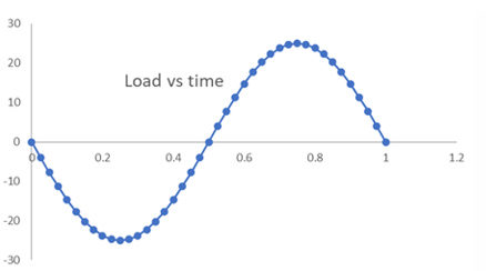
The cyclic-loading in this case requires many closely-spaced defined time points to describe the sinusoidal loading. A smooth transition occurs from one defined point to the next.
The default time-stepping behavior would therefore be inappropriate, as the time-stepping increments may be much smaller than desired because each defined time point is respected. Also, the default predictor behavior is unnecessary in this case because the load transition is smooth.
In such a scenario, it is appropriate to modify cyclic-loading behavior so that the defined table time points do not dictate time-stepping nor disable the predictor at those points (CLOAD,LTAB). Setting cyclic-loading in such a way ensures that the time-stepping command (NSUBST or DELTIM) dictates the time-stepping increments and not the defined time points. Defined time points may therefore be missed, and the predictor is not disabled even if the time points are hit.
If you require that defined time points are not missed but still want the predictor to remain enabled at those points, you can set the predictor to do so (PRED,ON,,ON). If both CLOAD,LTAB and PRED,ON,,ON are defined, the program considers the one defined most recently to control cyclic-loading behavior.
If the loading cycles have nonuniform time-point ranges, default time-stepping behavior can lead to an excessive number of substeps and longer run times.
In such cases, you can set time-stepping to apply
to each time-point range ( in the figure) in a cycle. If you enable this option
(CLOAD,TSTEP), time-stepping resets at each time-point
defined in the cyclic-loading table. The defined time points are always
respected.
in the figure) in a cycle. If you enable this option
(CLOAD,TSTEP), time-stepping resets at each time-point
defined in the cyclic-loading table. The defined time points are always
respected.
Example 6.5: Defining Time-Stepping Parameters for a Time-Point Range
CLOAD,TSTEP    ! enable time-point range time-stepping
NSUBST,1,20,1  ! time-stepping command
By default, the program disables the predictor at each defined table time point. You can set the predictor to remain enabled if desired (PRED,ON,,ON).
Writing all results for all substeps can lead to very large results (.rst) files.
To reduce the .rst file size, you can set output for specific time points only (CLOAD,OUTR), such as A and B in Figure 6.1: Time Points and Ranges in a Cyclic-Loading Table. Used with the key-time array option (OUTRES,,%array%), defined output points are required for only one cycle.
If you limit output to specific time points, results are output for each cycle by default. You can adjust the results frequency to output results at a specified cycle frequency (for example, every 10 cycles). Any key-time array point defined must also be a defined time-point in the cyclic-loading table.
Example 6.6: Selecting Output Time Points
*dim,timvals,array,2
timvals(1)=0.25
timvals(2)=1.2
OUTRES,ALL,%timvals%
CLOAD,OUTR,10   ! output every 10 cycles
Initiate the solution process (SOLVE). The program repeats the loading cycles for the specified number of times. The final solution time is therefore CYCTIME x CYCNUM. Do not enter a time value (TIME) for a cyclic-loading analysis solution.
Each cyclic-loading analysis solution occurs in a single load step with multiple substeps. All cycles are part of the same load step.
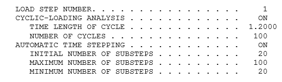
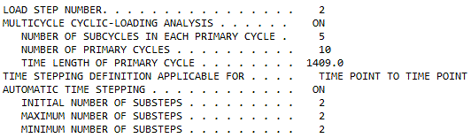
Load-step output includes information about the cyclic-loading analysis:
A cyclic-loading solution can be combined with a standard analysis solution in any order and combination. Different cyclic-loading solutions can have different cycle lengths. A single analysis can include multiple solutions of either type. For a standard solution, input the end time of the solution (TIME); otherwise, the program increments the prior load-step time value by 1.
If your analysis has multiple cyclic-loading solutions, be sure to perform the following tasks for each solution before issuing its associated SOLVE command:
Example 6.7: Cyclic Loading and Standard Solutions in a Single Analysis
! Load step 1: Standard SOLVE
! define solution options
…
TIME, 500
SOLVE

! Load step 2: Cyclic-Loading SOLVE
! define solution options
…
! apply cyclic load table(s)
NSEL, S, LOC, Y, 10
D,All,UY,%_cycload1%

CLOAD,CYCNUM,10
CLOAD,CYCTIME,20   ! No TIME command entered
SOLVE

! Load step 3: Cyclic-Loading SOLVE
! define solution options
…
! apply cyclic load table(s)
NSEL, S, LOC, Y, 10
D,All,UY,%_cycload1%

CLOAD,CYCNUM,5
CLOAD,CYCTIME,20   ! No TIME command entered
SOLVE

! Load step 4: Standard SOLVE
! define solution options
…
TIME, 900
SOLVE
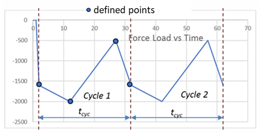
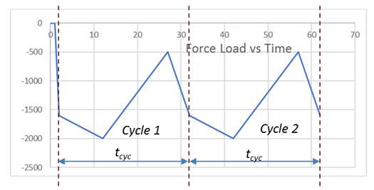
All loads such as degree-of-freedom constraints, forces, surface loads, and body force loads can be used for cyclic loading. The load must be entered as table. The start and end load values of the load table should be the same to prevent unexpected large load increments when cyclic loading occurs.
In this figure, the applied force load is ramped up to the starting value of the cyclic loading, and the cyclic loading has identical beginning and ending values:
A cyclic-loading analysis can be performed independent of a cycle-jump analysis .
The multicycle cyclic-loading analysis is useful for defining the fatigue load table for applications such as rainflow counting. This method allows for the primary cyclic-loading table to have subcycles, with each subcycle having its own number of cycles. Furthermore, the primary cycle can have its own number of cycles.
The following topics are available for multicycle cyclic-loading analysis:
Consider this cyclic-loading table consisting of a primary cycle and a number of subcycles:
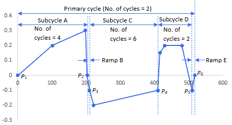
Subcycle A: From time-point P1 to P2. Number of cycles = 4.
Ramp B: From time-point P2 to P3.
Subcycle C: From time-point P3 to P4. Number of cycles = 6.
Subcycle D: From time-point P4 to P5. Number of cycles = 2.
Ramp E: From time-point P5 to P6.
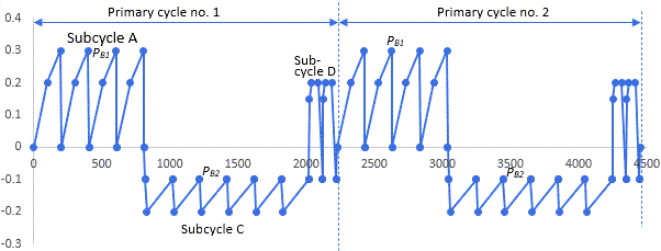
The multicycle cyclic-loading table example is equivalent to the following loading:
Loading for a multicycle cyclic-loading solution is possible by stitching together multiple standard cyclic-loading solutions and standard analysis solutions. Doing so, however, requires multiple SOLVE commands, one for each load step.
With the multicycle cyclic-loading method, the entire solution occurs in a single load step requiring one SOLVE command, leading to a more efficient, less computationally demanding solution.
Performing a multicycle cyclic-load analysis is similar to performing a standard cyclic-loading analysis with several key differences.
The following steps are involved in a multicycle cyclic-loading analysis:
- 6.1.2.2.1. Step 1: Define the Tabular Array
- 6.1.2.2.2. Step 2: Specify the Cyclic-Loading Table Values
- 6.1.2.2.3. Step 3: Apply the Cyclic-Loading Table(s)
- 6.1.2.2.4. Step 4. Specify Cyclic-Loading Parameters
- 6.1.2.2.5. Step 5. Specify Time-Stepping Parameters
- 6.1.2.2.6. Step 6. Select Output Time Points
- 6.1.2.2.7. Step 7. Solve the Cyclic-Loading Analysis
An additional dimension is required in the multicycle table to define the number of cycles for each subcycle. Set the second dimension to 2 (*DIM).
Example 6.8: Defining Multicycle Cyclic-Loading Tables
CLOAD,DEFINE,BEGIN
*DIM,_cycload1,TABLE,16,2
*DIM,_cycload2,TABLE,16,2
CLOAD,DEFINE,END
Multicycle cyclic-loading tables to be applied in the same cyclic-loading load step must have the same dimensions.
Load tables not specified as cyclic-loading tables (CLOAD,DEFINE) as shown are not cyclically repeated.
The multicycle table data is input into a single table. Column 0 contains the time-points, column 1 contains the load values, and column 2 contains the number of cycles for each subcycle.
Specifying the time values:
| The table time value must start at 0. Each subcycle time value must start at 0, and each new 0 represents a new subcycle. |
| Example: The time values for five subcycles are specified, with values of 0 specified at each new subcycle. |
Specifying the load values:
| The starting and ending load values of the primary cycle must be identical. |
| Example: Load values _cycload2(1 ,1) and _cycload2(16 ,1) are the same. |
| The ending load value of each subcycle must be the same as the starting load value of the next subcycle. |
| Example: The ending load value of the first subcycle _cycload2(4 ,1) is the same as the starting load value of the second subcycle _cycload2(5 ,1). The ending load value of the second subcycle _cycload2(6 ,1) is the same as the starting load value of the third subcycle _cycload2(7 ,1), and so on. |
| Ramp loads are input as part of the multicycle table. |
| For example, as shown in Figure 6.5: Multicycle Cyclic-Loading Example, there is a ramp load from P2 to P3. The ramp is specified in the input below as the time values _cycload2(5 ,0) to _cycload2(6 ,0), and load values _cycload2(5 ,1) to _cycload2(6 ,1). |
Specifying the number of cycles for each subcycle:
| The number of cycles information is specified in the column index 2 position. The row index at which each subcycle cycle number is specified corresponds to the row index value at the beginning of each subcycle. |
| Example: For subcycle 1, the row index value for the start of the subcycle is 1, so the number of cycles is set at _cycload2(1 ,2). For subcycle 2, the row index value for the start of the subcycle is 5, so the number of cycles is set at _cycload2(5 ,2), and so on. |
| For ramp loads, the number of cycles must be assigned a value of -1. This value allows the program to distinguish it from a regular subcycle. |
Example 6.9: Specifying Values in a Multicycle Cyclic-Loading Table
! Multicycle table !

! Time values
_cycload2(1 ,0) = 0      ! Time must start at 0.0
_cycload2(2 ,0) = 101
_cycload2(3 ,0) = 198
_cycload2(4 ,0) = 203

_cycload2(5 ,0) = 0      ! New 0 signifies new subcycle
_cycload2(6 ,0) = 7

_cycload2(7 ,0) = 0      ! New 0 signifies new subcycle
_cycload2(8 ,0) = 12
_cycload2(9 ,0) = 200

_cycload2(10,0) = 0      ! New 0 signifies new subcycle
_cycload2(11,0) = 5.5
_cycload2(12,0) = 20
_cycload2(13,0) = 70.3
_cycload2(14,0) = 100

_cycload2(15,0) = 0      ! New 0 signifies new subcycle
_cycload2(16,0) = 8

! Load values
_cycload2(1 ,1) = 0
_cycload2(2 ,1) = 0.2
_cycload2(3 ,1) = 0.3
_cycload2(4 ,1) = 0      ! End of subcycle value must match next value at start

_cycload2(5 ,1) = 0      ! Start of subcycle
_cycload2(6 ,1) = -0.1
_cycload2(7 ,1) = -0.1
_cycload2(8 ,1) = -0.2
_cycload2(9 ,1) = -0.1
_cycload2(10,1) = -0.1
_cycload2(11,1) = 0.15
_cycload2(12,1) = 0.2
_cycload2(13,1) = 0.2
_cycload2(14,1) = -0.1
_cycload2(15,1) = -0.1
_cycload2(16,1) = 0      ! End value must match start value

! Number of cycles for each subcycle value
! The index values correspond to index values at new 0 time values
_cycload2(1 ,2) = 4
_cycload2(5 ,2) = -1     ! Ramp load--table values do not end in the same loading value
_cycload2(7 ,2) = 6
_cycload2(10 ,2) = 2
_cycload2(15 ,2) = -1    ! Ramp load
If a cyclic-loading load step has multiple cyclic-loading tables, each must have the same time values. Therefore, if there are multiple multicycle cyclic-loading tables in a given cyclic-loading load step, each must have the same subcycle number of cycles data as well.
Apply the multicycle loading tables as you would in a standard cyclic-loading analysis.
Unlike a standard cyclic-loading analysis, the length of the primary loading cycle is not specified and CLOAD,CYCTIME is not used. Instead, the program determines the length of the primary loading cycle based on the table time values and the number of cycles of each subcycle.
Set the number of subcycles for a multicycle cyclic-loading load step (CLOAD,MSUB). Setting this value is necessary only once per multicycle cyclic-loading load step, even multiple tables exist in the same load step.
Define the total number of cycles for the primary cycle (CLOAD,CYCNUM).
Example 6.10: Defining Cyclic-Loading Parameters
CLOAD,MSUB,5      ! Define number of subcycles
CLOAD,CYCNUM,10   ! total number of primary cycles
Specify the time-stepping parameters as you would for a standard cyclic-loading solution.
You can set the output for specific time points only, similar to a standard cyclic-loading solution.
For a multicycle solution, the time values in the key-time array option are with respect to the primary cycle. That is, although you enter the information for the multicycle table only as shown in Figure 6.5: Multicycle Cyclic-Loading Example, any time value specified must be as shown in Figure 6.6: Cyclic-Loading Example.
Specify the time value for the first primary cycle only. The time values should be less than the time length of the primary cycle.
Calculate the time values manually (with respect to time 0) for which outputs are desired, as they may not be values specified when defining the multicycle table.
| For example, as shown Figure 6.6: Cyclic-Loading Example, specify only the time value PB1 in the first primary cycle; the results are output in subsequent cycles at the same relative value PB1. The same applies for PB2. |
Depending on the time points you specify for output (CLOAD,OUTR), results are output at the specified frequency with respect to the primary cycle.
Example 6.11: Selecting Output Time Points
*dim,timvals,array,2
timvals(1)= 710     ! absolute value in 1st primary cycle
timvals(2)= 1224    ! absolute value in 1st primary cycle
OUTRES,ALL,%timvals%
CLOAD,OUTR,5   ! output every 5 cycles wrt the primary cycle
Initiate the solution as you would for a standard cyclic-loading analysis.
You can combine a multicycle cyclic-loading solution with a standard solution and/or a standard cyclic-loading solution in any order and combination.
A multicycle cyclic-loading analysis cannot be combined with a cycle-jump analysis.
A multiframe restart can resume a job at any point in a cyclic-loading analysis for which information is saved. The program will automatically complete the cyclic-loading analysis until the cyclic-loading end point. For example, if the cyclic-loading analysis consists of 100 cycles and the restart point is at some location in the 60th cycle, the restart analysis will commence at the restart point and run until the 100th cycle.
The following is an example of a typical multiframe restart of a cyclic-loading analysis.
Example 6.13: Multiframe Restart of a Cyclic-Loading Analysis
/SOLU
...

! Define cload table
...

! Apply cyclic load table
nsel,s,loc,z,1
sf,all,pres,%_cycload%
allsel

! Solution parameters
OUTRES,ALL,ALL
nsubst,20,100,8
...

! Define cyclic loading analysis parameters
CLOAD,CYCNUM,5
CLOAD,CYCTIME,2.5

! Restart parameters
!RESCONTROL, Action, Ldstep, Frequency, MAXFILES,
rescontrol,        ,    2,       25,
solve

rescontrol,file_summary
save,file,db

finish

!*************** RESTART ***************
/clear,nostart
resume,file,db
finish

/solu
! Restart point
antype,static,restart,2,25,continue

allsel
solve
finish
The following limitations apply to cyclic loading:
A multicycle cyclic-loading analysis does not support restart.