


The program uses real constants and KEYOPTs to control contact behavior using surface-to-surface contact elements. For more information in addition to what is presented here, refer to the individual contact element descriptions in the Element Reference.
If you decide the real constant and KEYOPT settings you have specified for a particular contact pair are not appropriate, you can use the CNCHECK,RESET command to reset all values back to their default settings. Some real constants and key options are not affected by this command. See CNCHECK for details.
In many cases, certain default settings may not be appropriate for your specific model. You can issue the CNCHECK,AUTO command to obtain optimized KEYOPT and real constant settings in terms of robustness and efficiency. Usually, only the undefined or default KEYOPT settings and real constants are changed. Refer to the CNCHECK command description for details of which settings are typically changed. You should always verify these changes by issuing the CNCHECK,DETAIL command to list current contact pair properties. If necessary, you can overwrite the optimized settings by redefining specific KEYOPTs (KEYOPT command) and real constants (RMODIF command).
The following related topics are available:
- 3.9.1. Real Constants
- 3.9.2. Element KEYOPTS
- 3.9.3. Selecting a Contact Algorithm (KEYOPT(2))
- 3.9.4. Determining Contact Stiffness and Allowable Penetration
- 3.9.5. Choosing a Friction Model
- 3.9.6. Selecting Location of Contact Detection
- 3.9.7. Selecting a Sliding Behavior
- 3.9.8. Adjusting Initial Contact Conditions
- 3.9.9. Modeling Interference Fit
- 3.9.10. Physically Moving Contact Nodes Toward the Target Surface
- 3.9.11. Physically Moving the Target Body Toward the Contact Surface
- 3.9.12. Determining Contact Status and the Pinball Region
- 3.9.13. Avoiding Spurious Contact in Self Contact Problems
- 3.9.14. Selecting Surface Interaction Models
- 3.9.15. Using KEYOPT(3) to Control Units of Contact Stiffness and Stress State
- 3.9.16. Modeling Contact with Superelements
- 3.9.17. Modeling Contact for 2D Axisymmetric Elements with Torsion
- 3.9.18. Applying Contact Stabilization Damping
- 3.9.19. Modeling Interface Damping in Assembled Structures
- 3.9.20. Accounting for Thickness Effect
- 3.9.21. Using Time Step Control and Impact Constraints
- 3.9.22. Using the Birth and Death Options
Use the R and RMORE commands to define real constants. The first two real constants, R1 and R2, are used to define the geometry of the target surface elements. The remaining are used by the contact surface elements.
R1 and R2 define the target element geometry.
FTOLN is a factor based on the thickness of the element which is used to calculate allowable penetration. [2]
ICONT defines an initial closure factor (or adjustment band).
PINB defines a "pinball" region.
PZER defines pressure at zero penetration.
CZER defines initial clearance.
TAUMAX specifies the maximum contact friction.
CNOF specifies the positive or negative offset value applied to the contact surface.
FKOP specifies the stiffness factor applied when contact opens.
COHE specifies the cohesion sliding resistance.
TCC specifies the thermal contact conductance coefficient.
FHTG specifies the fraction of frictional dissipated energy converted into heat.
SBCT specifies the Stefan-Boltzmann constant.
RDVF specifies the radiation view factor.
FWGT specifies the weight factor for the distribution of heat between the contact and target surfaces for thermal contact or for electric contact.
ECC specifies the electric contact conductance or capacitance per unit area.
FHEG specifies the fraction of electric dissipated energy converted into heat.
FACT specifies the ratio of static to dynamic coefficients of friction.
DC specifies the decay coefficient for static/dynamic friction.
SLTO controls maximum sliding distance when MU is nonzero and the tangent contact stiffness (FKT) is updated at each iteration (KEYOPT(10) = 0 or 2) or when KEYOPT(2) = 3.
TNOP specifies the maximum allowable tensile contact pressure. [2]
TOLS adds a small tolerance that extends the edge of the target surface.
MCC specifies the magnetic contact permeance (3D only).
PPCN specifies the pressure-penetration criterion (surface contact elements only).
FPAT specifies the fluid penetration acting time (surface contact elements only).
COR specifies the coefficient of restitution for impact between rigid bodies using impact constraints (KEYOPT(7) = 4).
STRM specifies load step number for ramping penetration, or starting time for ramping contact stiffness.
FDMN specifies the stabilization damping factor in the normal direction.
FDMT specifies the stabilization damping factor in the tangential direction.
FDMD specifies the destabilizing squeal damping factor (3D only).
FDMS specifies the stabilizing squeal damping factor (3D only).
TBND specifies the critical bonding temperature.
WBID is an internal contact pair ID (used only by the Results Tracker in Workbench Mechanical)
PCC specifies the pore fluid contact permeability coefficient.
PSEE specifies the pore fluid seepage.
ABPP specifies the ambient pore pressure.
FPFT specifies the gap pore fluid flow participation factor.
FPWT specifies the gap pore fluid flow distribution weighting factor.
DCC specifies the diffusivity coefficient.
DCON specifies the diffusive convection coefficient.
ABDC specifies the ambient concentration.
BSRL identifies the real constant set ID of the original (base) contact pair after a spitting operation.
KSYM identifies the real constant set ID of the companion pair for a symmetric pair or self contact (determined by the splitting logic).
TFOR specifies the pair-based force convergence tolerance.
TEND defines the ending time for ramping contact stiffness.
When the contact element is used as part of a forced-distributed constraint and KEYOPT(7) = 2 on the target element, FKN is used to define weighting factors in tabular format with node number as the primary variable.
When the relaxation option is enabled (KEYOPT(11) = 1 on the target element) for a surface-based constraint or a rigid body, FKN and FKT are translational relaxation coefficient and rotational relaxation coefficient, respectively, and tabular input is not supported. In addition, FTOLN and TNOP are translational tolerance and rotational tolerance, respectively.
Real constant defaults can vary depending on the environment you are working in. The following table compares the program default values with those of the Ansys Workbench product.
Table 3.1: Summary of Real Constant Defaults in Different Environments
| Real Constants | Description | Ansys Mechanical APDL Default | Ansys Workbench Default | |
|---|---|---|---|---|
| No. | Name | |||
| 1 | R1 [4] | Radius associated with target geometry |
0 | n/a |
|
Target radius (CONTA177) |
Calculated by program | |||
| 2 | R2 [4] |
Radius associated with target geometry |
0 | n/a |
|
Superelement thickness |
1 | |||
|
Contact radius (CONTA177) |
Calculated by program | |||
| 3 | FKN | Normal penalty stiffness factor | 1 | [1] |
| 4 | FTOLN | Penetration tolerance factor | 0.1 | 0.1 |
| 5 | ICONT | Initial contact closure | 0 | 0 |
| 6 | PINB | Pinball region | [2] | [2] |
| 7 | PZER | Pressure at zero penetration | [7] | [7] |
| 8 | CZER | Initial contact clearance factor | 0.01 | 0.01 |
| 9 | TAUMAX | Maximum friction stress | 1.00E+20 | 1.00E+20 |
| 10 | CNOF | Contact surface offset | 0 | 0 |
| 11 | FKOP | Contact opening stiffness | 1 | 1 |
| 12 | FKT | Tangent penalty stiffness factor | 1 | 1 |
| 13 | COHE | Contact cohesion | 0 | 0 |
| 14 | TCC | Thermal contact conductance | 0 | [3] |
| 15 | FHTG | Frictional heating factor | 1 | 1 |
| 16 | SBCT | Stefan-Boltzmann constant | 0 | n/a |
| 17 | RDVF | Radiation view factor | 1 | n/a |
| 18 | FWGT | Heat distribution weighing factor | 0.5 | 0.5 |
| 19 | ECC | Electric contact conductance | 0 | [6] |
| 20 | FHEG | Joule dissipation weighting factor | 1 | n/a |
| 21 | FACT | Static/dynamic ratio | 1 | 1 |
| 22 | DC | Exponential decay coefficient | 0 | 0 |
| 23 | SLTO | Allowable elastic slip | 1% | 1% |
| 24 | TNOP | Maximum allowable tensile contact pressure | [5] | [5] |
| 25 | TOLS | Target edge extension factor | 2 | 2 |
| 26 | MCC | Magnetic contact permeance | 0 | n/a |
| 27 | PPCN | Pressure-penetration criterion | 0 | n/a |
| 28 | FPAT | Fluid penetration acting time | 0.01 | n/a |
| 29 | COR | Coefficient of restitution | 1 | 1 |
| 30 | STRM | Load step number for ramping penetration | 1 [8] | 1 [8] |
| 31 | FDMN | Normal stabilization damping factor | 1 | n/a |
| 32 | FDMT | Tangential stabilization damping factor | 0.001 | n/a |
| 33 | FDMD | Destabilizing squeal damping factor | 1 | n/a |
| 34 | FDMS | Stabilizing squeal damping factor | 0 | n/a |
| 35 | TBND | Critical bonding temperature | n/a | n/a |
| 36 | WBID | Internal contact pair ID (used only by the Results Tracker in Workbench Mechanical) | n/a | Internal pair ID |
| 37 | PCC | Pore fluid contact permeability coefficient | 0 | n/a |
| 38 | PSEE | Pore fluid seepage coefficient | 0 | n/a |
| 39 | ABPP | Ambient pore pressure | 0 | n/a |
| 40 | FPFT | Gap pore fluid flow participation factor | 0 | n/a |
| 41 | FPWT | Gap pore fluid flow distribution weighting factor | 0.5 | n/a |
| 42 | DCC | Contact diffusivity coefficient | 0 | n/a |
| 43 | DCON | Diffusive convection coefficient | 0 | n/a |
| 44 | ABDC | Ambient concentration | 0 | n/a |
| 45 | BSRL | Real ID of base contact pair (after splitting) | 0 | n/a |
| 46 | KSYM | Real ID of companion pair (determined by the splitting logic) | 0 | n/a |
| 47 | TFOR | Pair-based force convergence tolerance | n/a | n/a |
| 48 | TEND | Ending time for ramping contact stiffness | 0 | 0 |
FKN = 10 for bonded. For all other, FKN = 1.0, but if bonded and other contact behavior exists, FKN = 1 for all.
Depends on contact behavior (rigid vs. flex target), NLGEOM,ON or OFF, KEYOPT(9) setting, KEYOPT(12) setting, and the value of CNOF (see Defining the Pinball Region (PINB)).
Calculated as a function of highest conductivity and overall model size.
R1 and R2 are used to define the contact or target element geometry for pair-based contact. See Defining Target Element Geometry and the target element descriptions (TARGE169 and TARGE170) for details on how they are used for different geometries.
TNOP defaults to the force convergence tolerance divided by contact area at contact nodes.
Calculated as a function of lowest resistivity and overall model size.
If TEND is specified as a positive value, STRM defaults to zero.
For the real constants FKN, FTOLN, ICONT, PINB, PZER, CZER, FKOP, FKT, SLTO, TNOP, FDMN, and FDMT, you can specify either a positive or negative value. The program interprets a positive value as a scaling factor and interprets a negative value as the absolute value. The program uses the depth of the underlying element as the reference value for ICONT, FTOLN, PINB, and CZER. For example, a positive value of 0.1 for ICONT indicates an initial closure factor of 0.1 x depth of the underlying element. However, a negative value of 0.1 indicates an actual adjustment band of 0.1 units. Contact related settings (ICONT, FTOLN, PINB, FKN, FKT, SLTO) are always averaged across all contact elements in a contact pair.
Figure 3.12: Depth of the Underlying Element shows the depth of the underlying element for a solid element. If the underlying elements are shell or beam elements, the depth will usually be 4 times the element thickness. The final contact depth may also be adjusted based on the average contact length when the shape of the underlying element is relatively thin.
Each contact pair has a pair-based depth which is obtained by averaging the depth of each contact element across all the contact elements in a contact pair. This can avoid the problem of very different element-based depths when there are meshes with large variations in element sizes.
Note: When the contact pair depth is too small (for example, 10-5), the machine precision may not guarantee the accuracy of penetration to be calculated. You should scale the length unit in the model.
For certain real constants, you can define the real constant as a function of primary variables by using tabular input. Table 3.2: Real Constants and Corresponding Primary Variables for CONTA172, CONTA174, CONTA175, CONTA177 lists real constants that allow tabular input and their associated primary variables.
You should follow the positive and negative convention for the real constant values. Use all positive or all negative values. Do not mix positive and negative values.
Use the *DIM command to dimension the table and identify the variables. The possible primary variables used in tabular input are:
Time (TIME)
X location (X) in local/global coordinates
Y location (Y) in local/global coordinates
Z location (Z) in local/global coordinates
Temperature (TEMP) degree of freedom
Contact pressure (PRESSURE):
Specify positive index values for compression, negative index values for tension.
Geometric contact gap/penetration (GAP):
Numerical offsets are not included.
Specify positive index values for penetration, negative index values for an open gap.
Node number (NODE)
Note that the primary variables X, Y, and Z represent the coordinates of the contact detection points at the beginning of solution (undeformed configuration). Coordinate system applicability is determined by the *DIM command.
When defining the tables, the primary variables must be in ascending order in the table indices (as in any table array).
When defining real constants via the R,
RMORE, or RMODIF command, enclose the
table name in % signs (that is, %tabname%). For
example, given a table named CNREAL3 that contains normal contact stiffness
(FKN) values, you would issue a command similar to the following:
RMODIF,NSET,3,%CNREAL3% !NSETis the real constant set ID associated with the contact pair
For more information and examples of using table inputs, see Tabular Input via Table Array Parameters in the Ansys Parametric Design Language Guide, Applying Loads Using Tabular Input in the Basic Analysis Guide, and the *DIM command.
Table 3.2: Real Constants and Corresponding Primary Variables for CONTA172, CONTA174, CONTA175, CONTA177
| Real Constants | TIME | Location (X,Y,Z) [1] | TEMP | PRESSURE [2] | GAP [3] | NODE | %_CNPROP% [6] | |
|---|---|---|---|---|---|---|---|---|
| Number | Name | |||||||
| 3 | FKN | x | x | x | x [4] | x | x [8] | x |
| 7 | PZER | x [7] | x [7] | |||||
| 9 | TAUMAX | x | x | x | x | x | x | |
| 10 | CNOF | x | x | x | ||||
| 11 | FKOP | x | x | x | x | x | ||
| 12 | FKT | x | x | x | x | x | x | |
| 14 | TCC | x | x | x | x [5] | x | x | |
| 17 | RDVF | x | x | x | x | x | ||
| 19 | ECC | x | x | x | x [5] | x | x | |
| 26 | MCC | x | x | x | x | x | ||
| 27 | PPCN | x | x | x | x | x | x | |
| 31 | FDMN | x | x | x | x | x | ||
| 32 | FDMT | x | x | x | x | x | ||
| 35 | TBND | x | x | x | x | x | x | |
| 37 | PCC | x | x | x | x [5] | x | x | |
| 38 | PSEE | x | x | x | x [5] | x | x | |
| 39 | ABPP | x | x | x | x [5] | x | x | |
| 40 | FPFT | x | x | x | x | x | x | |
| 42 | DCC | x | x | x | x [5] | x | x | |
| 43 | DCON | x | x | x | x [5] | x | x | |
| 44 | ABDC | x | x | x | x [5] | x | x | |
Coordinates of the contact detection points at the beginning of solution (undeformed configuration).
Contact normal pressure via the primary variable PRESSURE. For PRESSURE index values, specify positive values for compression or negative value for tension.
Geometric contact gap/penetration via the primary variable GAP. For GAP index values, specify positive values for penetration or negative values for an open gap.
Contact pressure at the end of the previous iteration, if it exists.
When the contact element type does not contain any structural degrees of freedom, the real constants TCC, ECC, PCC, PSEE, ABPP, DCC, DCON, and ABDC should not be defined as a function of the contact pressure.
When defined by tabular input or by the
USERCNPROP.Fuser subroutine, PZER must be a positive value, and it represents an absolute pressure (not a factor). This differs from its typical usage.When the contact element is used as part of a forced-distributed constraint and KEYOPT(7) = 2 on the target element, FKN is used to define weighting factors in tabular format with node number as the primary variable.
You can write a USERCNPROP.F subroutine to define your
own real constants. The real constants that can be defined via this user
subroutine are noted in the real constant table found in each contact element
description.
When defining real constants with the R,
RMORE, or RMODIF command, you must use
the reserved table name _CNPROP and enclose it in % signs (%_CNPROP%). When a
value field on one of these commands is set to %_CNPROP%, the program internally
calls the user-defined subroutine USERCNPROP. For example,
to specify your own normal contact stiffness, FKN, you would issue a command
similar to the following:
RMODIF,NSET,3,%_CNPROP% !NSETis the real constant set ID associated with the contact pair
If several real constant values are defined via %_CNPROP% for a given contact
pair, the subroutine will be called for each of these real constant entries.
Therefore, you can use a single USERCNPROP subroutine to
modify multiple real constant values. For details, see Defining Your Own Real Constant (USERCNPROP).
Each contact element includes several KEYOPTS. Ansys recommends using the default settings, which are suitable for most contact problems. For some specific applications, you can override the defaults. The element KEYOPTS allow you to control several aspects of contact behavior.
KEYOPT defaults can vary depending on the environment you are working in. The following table compares the default values between the various contact creation tools, for both Ansys Mechanical APDL and Ansys Workbench.
Table 3.3: Summary of KEYOPT Defaults in Different Environments
| KEYOPT | Description | Ansys Mechanical APDL | Contact Wizard | General Contact (GCGEN command) | Ansys Workbench Default Linear (bonded, no sep) | Ansys Workbench, Default Nonlinear (standard, rough) |
|---|---|---|---|---|---|---|
| 1 | Selects DOF [1] | Manual | Auto | Auto | Auto | Auto |
| 2 | Contact Algorithm | Aug. Lagr. | Aug. Lagr. | Penalty | Aug. Lagr. | Aug. Lagr. |
| 3 | Unit control for normal contact stiffness or 2D stress state for underlying superelements | No unit control | No unit control | Not supported | n/a | n/a |
| 4 | Location of contact detection point | gauss | gauss | gauss | gauss | gauss |
| 5 | CNOF/ICONT adjustment | No adjust | No adjust | Not supported | No adjust | No adjust |
| 6 | Contact stiffnes variation | Use default range | Use default range | Use default range | Use default range | Use default range |
| 7 | Element level time increment control | No control | No control | No control | No control | No control |
| 8 | Symmetric contact behavior | No action | No action | GCDEF option | No action | No action |
| 9 | Effect of initial penetration or gap | Include all | Include all | TBDATA,,C1 | Exclude all | Include all |
| 10 | Contact stiffness update | Between iterations | Between iterations | Between iterations | Between iterations | Between iterations |
| 11 | Beam/shell thickness effect | Exclude | Exclude | Include | Exclude | Exclude |
| 12 | Behavior of contact surface | Standard | Standard |
TB,INTER,,,TBOPT | Bonded | n/a |
| 13 | Degree-of-freedom control for contact involving thermal shells | TEMP degree of freedom | n/a | Not supported | n/a | n/a |
| 14 | Behavior of fluid penetration load | Iteration- based | Iteration- based | Not supported | n/a | n/a |
| 15 | Effect of stabilization damping | Active only in first load step | n/a | Active only in first load step | n/a | n/a |
| 16 | Squeal damping controls | Damping scaling factor | n/a | Not supported | n/a | n/a |
| 18 | Sliding behavior | Finite sliding | Finite sliding | Finite sliding | Small sliding [2] | Finite sliding [3] |
For surface-to-surface contact elements, the program offers several different contact algorithms:
Penalty method (KEYOPT(2) = 1)
Augmented Lagrangian (default) (KEYOPT(2) = 0)
Lagrange multiplier on contact normal and penalty on tangent (KEYOPT(2) = 3)
Pure Lagrange multiplier on contact normal and tangent (KEYOPT(2) = 4)
Internal multipoint constraint (MPC) (KEYOPT(2) = 2)
The penalty method uses a contact spring to establish a relationship between the two contact surfaces. The spring stiffness is called the contact stiffness. This method uses the following real constants: FKN and FKT for all values of KEYOPT(10), plus FTOLN and SLTO if KEYOPT(10) = 0 or 2.
The augmented Lagrangian method (which is the default) is an iterative series of penalty methods. The contact tractions (pressure and frictional stresses) are augmented during equilibrium iterations so that the final penetration is smaller than the allowable tolerance (FTOLN). Compared to the penalty method, the augmented Lagrangian method usually leads to better conditioning and is less sensitive to the magnitude of the contact stiffness. However, in some analyses, the augmented Lagrangian method may require additional iterations, especially if the deformed mesh becomes too distorted.
The pure Lagrange multiplier method enforces zero penetration when contact is closed and "zero slip" when sticking contact occurs. The pure Lagrange multiplier method does not require contact stiffness, FKN and FKT. Instead it requires chattering control parameters, FTOLN and TNOP. This method adds contact traction to the model as additional degrees of freedom and requires additional iterations to stabilize contact conditions. It often increases the computational cost compared to the augmented Lagrangian method.
An alternative algorithm is the Lagrange multiplier method applied on the contact normal and the penalty method (tangential contact stiffness) on the frictional plane. This method enforces zero penetration and allows a small amount of slip for the sticking contact condition. It requires chattering control parameters, FTOLN and TNOP, as well as the maximum allowable elastic slip parameter SLTO.
The internal multipoint constraint (MPC) algorithm is used in conjunction with bonded contact (KEYOPT(12) = 5 or 6) and no separation contact (KEYOPT(12) = 4) to model several types of contact assemblies and kinematic constraints. See Multipoint Constraints and Assemblies for more information about how to use this feature.
Keep the following points in mind when using the Lagrange multiplier methods.
The Lagrange multiplier methods (KEYOPT(2) = 3, 4) do not support the Gauss point detection option (KEYOPT(4) = 0) for surface-to-surface contact. They support the nodal detection options for surface-to-surface contact and node-to-surface contact. When using these options, be careful not to overconstrain the model. The model is overconstrained when a contact node has prescribed boundary conditions, CE equations, or CP equations. The program first attempts to detect all potential overconstraints, and then eliminates the overconstraints by switching to the penalty method internally. However, there is no guarantee that the program will eliminate all cases of overconstraint. You should always verify your model carefully to address this issue.
For 3D higher-order contact elements (CONTA174) using nodal detection (KEYOPT(4)=1,2), the Lagrange multiplier method is applied at each contact node (including midside nodes), but the penalty method is applied on the center of the contact elements, even when KEYOPT(2) = 3 or 4 is set. For Normal Lagrange formulation (KEYOPT(2)=3,4), with 3D higher-order contact elements (with midside nodes), use of surface projection-based contacts (KEYOPT(4)=3,4) is strongly recommended.
In general, normal contact stiffness (FKN) has very little influence on the contact results when a Lagrange multiplier method is used. You should not overwrite the default FKN in most cases.
The Lagrange multiplier methods also introduce more degrees of freedom, which may result in spurious modes for modal and linear eigenvalue buckling analyses. The augmented Lagrangian method (KEYOPT(2) = 0) would be a better choice for these analysis types.
The Lagrange multiplier methods introduce zero diagonal terms in the stiffness matrix. Any iterative solver (for example, the PCG solver) will encounter a preconditioning matrix singularity with these methods. Therefore, you should switch to the sparse solver.
The following topics related to determining contact stiffness and allowable penetration are available.
For the augmented Lagrangian method and penalty method, normal and tangential contact stiffnesses are required. The amount of penetration between contact and target surfaces depends on the normal stiffness. The amount of slip in sticking contact depends on the tangential stiffness.
Higher stiffness values decrease the amount of penetration/slip, but can lead to ill-conditioning of the global stiffness matrix and to convergence difficulties. Lower stiffness values can lead to a certain amount of penetration/slip and produce an inaccurate solution. Ideally, you want a high enough stiffness that the penetration/slip is acceptably small, but a low enough stiffness that the problem will be well-behaved in terms of convergence.
The program provides default values for contact stiffnesses (FKN, FKT), allowable penetration (FTOLN), and allowable slip (SLTO). Material properties of underlying elements can affect the calculation of default values of contact stiffnesses, as follows:
If the underlying solid material is an anisotropic elastic material, all elastic moduli may affect the contact stiffness.
The initial contact stiffness of contact elements overlaid on layered structural solid elements (SOLID185 or SOLID186) is influenced by the material properties of each layer weighted by the respective layer thickness.
In most cases, you do not need to define the contact stiffness. In addition, Ansys recommends that you use KEYOPT(10) = 0 or 2 to allow the program to update the contact stiffness automatically.
For certain contact problems, you may choose to use the real constant FKN to define a normal contact stiffness factor. The usual factor range is from 0.1 - 10.0, with a default of 1.0. The default value should work in most cases. You can also define an absolute normal contact stiffness by specifying a negative value for FKN.
In addition, FKN can be defined as a function of primary variables by using
tabular input (%tabname%). The possible primary
variables include time, temperature, initial contact detection point location
(at the beginning of solution), contact pressure of the previous iteration
(positive PRESSURE index values indicate compression, negative PRESSURE index
values indicate tension), and current geometric penetration (positive GAP index
values indicate penetration, negative GAP index values indicate an open gap).
For more information, see Defining Real Constants in Tabular Format.
The user subroutine USERCNPROP.F is also available for
defining FKN. To use this subroutine, you must specify the table name %_CNPROP%
as the real constant value. For more information, see Defining Real Constants via a User Subroutine.
If you input an absolute normal contact stiffness by specifying a negative value for FKN, you can control the units by using KEYOPT(3). By default, the units of the user-specified absolute normal contact stiffness is FORCE/LENGTH3. You can change the units to FORCE/LENGTH by setting KEYOPT(3) = 1. This KEYOPT(3) = 1 setting is valid only when a penalty-based algorithm is used (KEYOPT(2) = 0 or 1) and the absolute normal contact stiffness is explicitly specified. Using KEYOPT(3) = 1 is not recommended in conjunction with nodal detection options (KEYOPT(4) = 1 or 2) if any midside nodes exist for the CONTA174 3D contact element. (KEYOPT(3) has different meanings in other situations. For more information, see Using KEYOPT(3) to Control Units of Contact Stiffness and Stress State.)
Note: The default contact normal stiffness is affected by defined material properties, element size, and the user-defined penetration tolerance (FTOLN). Many factors may be applied to the actual contact normal stiffness during the solution. The default contact stiffness listed in the Contact Manager or by the CNCHECK command may be different from the actual contact stiffness reported by the ETABLE command. You should check the value reported by ETABLE to confirm that the appropriate contact normal stiffness is used.
Use real constant FTOLN in conjunction with the augmented Lagrangian method. FTOLN is a tolerance factor to be applied in the direction of the surface normal. The range for this factor is less than 1.0 (usually less than 0.2), with a default of 0.1, and is based on the depth of the underlying solid, shell, or beam element (see Figure 3.12: Depth of the Underlying Element). This factor is used to determine if penetration compatibility is satisfied.
Contact compatibility is satisfied if penetration is within an allowable tolerance (FTOLN times the depth of underlying elements). The depth is defined by the average depth of each individual contact element in the pair. If the program detects any penetration larger than this tolerance, the global solution is still considered unconverged, even though the residual forces and displacement increments have met convergence criteria. You can also define an absolute allowable penetration by specifying a negative value for FTOLN. In general, the default contact normal stiffness is inversely proportional to the final penetration tolerance. The tighter the tolerance, the higher the contact normal stiffness.
When you use real constant FTOLN in conjunction with KEYOPT(10) = 0 or 2, the normal contact stiffness (used for the penalty method and the augmented Lagrange method) is updated at each iteration based on the current mean stress of the underlying elements and the allowable tolerance (FTOLN times the depth of the underlying elements). See also Using KEYOPT(10).
Note: When the contact stiffness is too large (for example, 1016), the machine precision may not guarantee good conditioning of the global stiffness matrix. In this case, you should scale the force unit in the model if possible.
Note: FTOLN is also used in the Lagrange multiplier methods (KEYOPT(2) = 3, 4) as a chattering control parameter.
The program automatically defines a default tangential contact stiffness that is proportional to MU and the normal stiffness FKN. The default tangential stiffness corresponds to a default value of FKT = 1.0. A positive value for FKT is a factor. A negative value indicates an absolute value of tangential stiffness.
For KEYOPT(10) = 0 or 2, or when the Lagrange multiplier on normal and penalty on tangent option is used (KEYOPT(2) = 3), the program updates tangential contact stiffness based on current contact normal pressure, PRES, and maximum allowable elastic slip, SLTO (KT = FKT*MU* PRES/SLTO). In addition, other adjustments may be applied to the tangential contact stiffness.
By default, the allowed tangential contact stiffness variation is intended to enhance stiffness updating (when KEYOPT(13) = 0) by calculating an optimal allowable range in stiffness for use in the updating scheme. To increase the tangential stiffness variational range for the frictional contact, set KEYOPT(13) = 1 to make an aggressive refinement to the allowable stiffness range. Use of KEYOPT(13) = 1 is not recommended when contact convergence is relatively easy as it might produce a large amount of elastic slip for sticking contact.
The real constant SLTO is used to control maximum sliding distance when FKT is updated at each iteration. The program provides default tolerance values which work well in most cases.
The default value for SLTO is 1 percent of the average contact length in a pair. However, for a steady-state rolling analysis, the default value is 0.1(ω*R), where ω is the spin velocity specified by the SSTATE command and R is the distance of the contact detection point from the center of rotation.
You can override the default value for SLTO by defining a scaling factor (positive value when using command input) or an absolute value (negative value when using command input). A larger value will enhance convergence but compromise accuracy. Based on the tolerance, current normal pressure, and friction coefficient, the tangential contact stiffness FKT can be obtained automatically. In certain cases users can override FKT by defining a scaling factor (positive input value) or absolute value (negative input value) (see Positive and Negative Real Constants for more information).
In addition, FKT can be defined as a function of primary variables by using
tabular input (that is, %tabname%). The possible
primary variables include time, temperature, initial contact detection point
location (at the beginning of solution), current contact pressure (positive
PRESSURE index values indicate compression, negative PRESSURE index values
indicate tension), and current geometric penetration (positive GAP index values
indicate penetration, negative GAP index values indicate an open gap). For more
information, see Defining Real Constants in Tabular Format.
The user subroutine USERCNPROP.F is also available for
defining FKT. To use this subroutine, you must specify the table name %_CNPROP%
as the real constant value. For more information, see Defining Real Constants via a User Subroutine.
FKN, FTOLN, FKT, and SLTO can be modified from one load step to another. They can also be adjusted in a restart run.
Determining a good stiffness value may require some experimentation on your part. To arrive at a good stiffness value, you can try the following procedure as a "trial run":
Use a low value for the contact stiffness to start. In general, it is better to underestimate this value rather than overestimate it. Penetration problems resulting from a low stiffness are easier to fix than convergence difficulties that arise from a high stiffness.
Run the analysis up to a fraction of the final load (just enough to get the contact fully established).
Check the penetration and the number of equilibrium iterations used in each substep. If the global convergence difficulty is caused by too much penetration (rather than by residual forces and displacement increments), FKN may be underestimated or FTOLN may be too small. If the global convergence requires many equilibrium iterations for achieving convergence tolerances of residual forces and displacements rather than the resulting penetration, FKN or FKT may be overestimated.
Adjust FKN, FKT, FTOLN, or SLTO as necessary and run the full analysis. If the penetration control becomes dominant in the global equilibrium iterations (that is, if more iterations were used to converge the problem to within the penetration tolerance than to converge the residual forces), you may increase FTOLN to permit more allowable penetration or increase FKN.
In addition, keep these points in mind when specifying contact stiffness:
For bonded contact and rough contact, the program uses MU = 1.0 to calculate tangential contact stiffness. The default tangential contact stiffness is proportional to the normal stiffness when the contact status is closed or open (near-field). When an absolute value of tangential stiffness is specified (a negative value input for FKT), the tangential stiffness remains unchanged regardless of the contact status.
Generally, the contact stiffness, FKN and FKT, has units of FORCE/LENGTH3. However, for contact force-based models the contact stiffness has units FORCE/LENGTH. This applies to CONTA175 with KEYOPT(3) = 0 and CONTA177 with KEYOPT(3) = 0 or 4. In addition, the absolute normal contact stiffness (that is, a negative value input for FKN) can have units of FORCE/LENGTH under some circumstances. See Using FKN and FTOLN for more information.
In general, if the underlying solid element has material properties defined by both TB and MP commands, the properties defined by TB take precedence over the properties defined by MP in the calculation of initial contact stiffness. However, for TB,EXPE (experimental data) and TB,USER (user-defined material model), MP,EX takes precedence. Ansys, Inc. recommends you define MP,EX when using TB,EXPE or TB,USER so that the initial contact stiffness is calculated using a realistic value for EX as defined by the MP command rather than a heuristic contact stiffness that is not influenced by the material property.
The normal and tangential contact stiffness can be updated during the course of an analysis, either automatically (due to large strain effects that change the underlying element's stiffness) or explicitly (by user-specified FKN or FKT values). KEYOPT(10) governs how the normal and tangential contact stiffness is updated when the augmented Lagrangian or penalty method is used. In most cases Ansys, Inc. recommends that you use KEYOPT(10) = 0 to allow the program to update contact stiffnesses automatically. The possible settings for KEYOPT(10) are:
KEYOPT(10) = 0: the normal contact stiffness is updated at each iteration based on the current mean stress of the underlying elements and the allowable penetration, FTOLN, except in the very first iteration. The default normal contact stiffness for the first iteration is determined by underlying element depth, material properties, and FTOLN. In addition, if bisections occur in the beginning of the analysis, the normal contact stiffness is reduced by a factor of 0.2 for each bisection. The tangential contact stiffness is updated at each iteration based on the current contact pressure, MU, and allowable slip (SLTO). The actual elastic slip never exceeds the maximum allowable limit (SLTO) during the entire solution.
KEYOPT(10) = 1: the contact stiffness is updated at each load step if FKN or FKT is redefined by the user. Stiffness and other settings (ICONT, FTOLN, SLTO, and PINB) are averaged across contact elements in a contact pair. The default contact stiffness is determined by underlying element depth and material properties.
KEYOPT(10) = 2: the behavior is similar to KEYOPT(10) = 0 (updating contact stiffness at each iteration), except that the actual elastic slip during the solution is guaranteed not to exceed the maximum allowable limit (SLTO) within a substep. In general, this option results in fewer iterations than the KEYOPT(10) = 0 option.
Note: When a Lagrange multiplier method (KEYOPT(2) = 4) or MPC algorithm (KEYOPT(2) = 2) is used, KEYOPT(10) is ignored.
The default method of updating normal contact stiffness (KEYOPT(10) = 0 or 2) is suitable for most applications. However, the variational range of the normal contact stiffness may not be wide enough to handle certain contact situations. For example:
In the case of a very small penetration tolerance (FTOLN), a larger normal contact stiffness is often needed.
If convergence difficulties are encountered (due to nonlinear materials, localized contact, etc.), a downward adjustment to stiffness may be helpful.
To stabilize the initial contact condition and to prevent rigid body motion, a smaller normal contact stiffness is required.
The allowed normal contact stiffness variation is intended to enhance stiffness updating when KEYOPT(10) = 0 or 2 by calculating an optimal allowable range in stiffness for use in the updating scheme. To increase the stiffness variational range, set KEYOPT(6) = 1 to make a nominal refinement to the allowable stiffness range, or KEYOPT(6) = 2 to make an aggressive refinement to the allowable stiffness range.
Use of KEYOPT(6) = 1 or 2 is not recommended when contact convergence is relatively easy as it might produce an unnecessary drop in contact stiffness.
Set KEYOPT(6) = 3 to define the pressure-penetration relationship. The augmented Lagrangian method (KEYOPT(2) = 0) with KEYOPT(6) = 3 behaves the same as the penalty algorithm (KEYOPT(2) = 1): no augmentation and penetration tolerance checks are applied. See Pressure-Penetration Relationship (KEYOPT(6) = 3) for more information.
When KEYOPT(6) = 0, 1, or 2, the program uses a uniform normal contact stiffness for each contact pair. This can cause convergence issues when the mesh size across contact elements within a pair varies greatly.
With the exponential pressure-penetration relationship (KEYOPT(6) = 3), the resulting contact stiffness is no longer uniform within a pair. This is a contact-detection-based law that can make contact behavior smoother in the following situations: self contact, contact involving soft materials like rubber, models having a large initial gap, non-uniform contact surface meshes, and contact interface chattering.
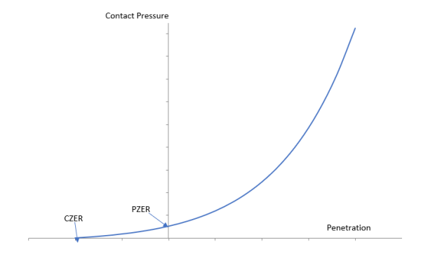
When KEYOPT(6) = 3, the contact pressure-penetration relationship follows an exponential law based on default values of real constants PZER (pressure at zero penetration) and CZER (initial contact clearance). PZER is calculated based on underlying element properties. A small contact pressure starts developing as the initial clearance is detected and increases exponentially as the gap reduces and penetration increases.
A positive value for CZER indicates a scaling factor associated with the depth of the underlying elements. A negative value indicates an absolute initial contact clearance value. CZER defaults to 0.01.
A positive value for PZER indicates a scaling factor, with the typical range being from 0.1 - 10.0. PZER default to 1.0. A negative value for PZER indicates an absolute contact pressure at zero penetration. When PZER is negative (an absolute value) and CZER is positive (a scaling factor), the program computes the actual contact pressure internally based on the penetration tolerance FTOLN and the initial contact clearance CZER.
The default values are adequate for most contact models. However, you can specify PZER and/or CZER to define the contact pressure-penetration exponential relationship.
You can also set a maximum cutoff stiffness by inputting real constant FKN. The computed contact stiffness from the exponential relationship will not exceed the cutoff value. If FKN is not specified, the program uses the default value of penalty contact stiffness to calculate the cutoff value. The actual cutoff stiffness is 1000 times the penalty stiffness input by you or computed by the program. For example, if FKN is not input and the program calculates an initial contact stiffness of 42265, the cutoff contact stiffness used is 0.42265E+08.
The following equation is used to define the contact stiffness vs. gap relationship (FKN as a function of gap, g):

where:
| c0 = initial gap |
| p = p0 when g = 0 |

Contact pressure can be defined as a function of gap by using tabular input (that
is, %tabname%) for real constant PZER with GAP as the
primary variable. GAP represents current geometric gap/penetration (positive GAP index
values indicate penetration, negative GAP index values indicate an open gap). For more
information, see Defining Real Constants in Tabular Format. Pressure will be 0 for gap greater
than CZER. Ansys recommends defining the table according to CZER.
Alternatively, you can use the user subroutine
USERCNPROP.F to define the pressure-gap
relationship. See Defining Your Own Real Constant (USERCNPROP) for details. To properly
define the relationship, be sure to return the following two output
arguments:
| cnprop(1) = user defined contact pressure at the given penetration |
| cnprop(2) = normal contact stiffness at the given penetration (derivative of the contact stiffness with respect to the penetration) |
When defined by tabular input or by the
USERCNPROP.F user subroutine, PZER must be a
positive value, and it represents an absolute pressure (not a factor). This
differs from its typical usage.
The pressure-penetration feature (KEYOPT(6) = 3):
Cannot be used with bonded and no-separation behaviors (KEYOPT(12) > 1).
Does not support the Lagrange methods and MPC contact (KEYOPT(2) > 1).
If the above settings are used, the program assumes aggressive-variation of contact stiffness (KEYOPT(6) = 2).
KEYOPT(6) = 3 does not support the Augmented Lagrange method (KEYOPT(2) = 0). If these settings are used together, the program switches to the penalty method (KEYOPT(2) = 1) internally.
When the automatic stiffness ramp-up option is defined (see 3. Automatically ramp up the contact stiffness under Modeling Interference Fit) the program internally actives the aggressive-variation of contact stiffness (KEYOPT(6) = 2) only for the specified load step or time period.
KEYOPT(6) = 3 is not recommended with the settings listed below since it may not behave as expected:
Impact constraints (KEYOPT(7) = 4)
Fluid penetration (SFE,,,PRES and KEYOPT(14))
In general, the Lagrange multiplier methods (KEYOPT(2) = 3, 4) do not require normal contact stiffness, FKN, unless overconstraints are detected. Instead they require chattering control parameters, FTOLN and TNOP, by which the program assumes that the contact status remains unchanged. FTOLN is the maximum allowable penetration and TNOP is the maximum allowable tensile contact pressure.
Note: A negative contact pressure occurs when the contact status is closed. A tensile contact pressure (positive) refers to a separation between the contact surfaces, but not necessarily an open contact status. However, the sign of the contact pressure is switched during postprocessing.
Note: For contact force-based models, TNOP is the maximum allowable tensile contact force. This applies to CONTA175 with KEYOPT(3) = 0 and CONTA177 with KEYOPT(3) = 0 or 4.
The behavior can be described as follows:
If the contact status from the previous iteration is open and the current calculated penetration is smaller than FTOLN, then contact remains open. Otherwise the contact status switches to closed and another iteration is processed.
If the contact status from the previous iteration is closed and the current calculated contact pressure is positive but smaller than TNOP, then contact remains closed. If the tensile contact pressure is larger than TNOP, then the contact status changes from closed to open and the program continues to the next iteration.
The program provides reasonable defaults for FTOLN and TNOP. FTOLN defaults to the displacement convergence tolerance. TNOP defaults to 1% of the force convergence tolerance divided by the contact area at contact nodes.
When providing values for FTOLN and TNOP:
A positive value is a scaling factor applied to the default values.
A negative value is used as an absolute value (which overrides the default).
The objective of FTOLN and TNOP is to provide stability to models which exhibit contact chattering due to changing contact status. If the values you use for these tolerances are too small, the solution will require more iterations. If the values are too large, however, the accuracy of the solution will be affected as a certain amount of penetration or tensile contact force is allowed.
The following topics related to choosing a friction model are available:
In the basic Coulomb friction model, two contacting surfaces can carry shear stresses up to a certain magnitude across their interface before they start sliding relative to each other. This state is known as sticking. The Coulomb friction model defines an equivalent shear stress τ, at which sliding on the surface begins as a fraction of the contact pressure p (τ = µp + COHE, where µ is the friction coefficient and COHE specifies the cohesion sliding resistance). Once the shear stress is exceeded, the two surfaces will slide relative to each other. This state is known as sliding. The sticking/sliding calculations determine when a point transitions from sticking to sliding or vice versa.
As an alternative to the program-supplied friction model, you can define your
own friction model with the USERFRIC subroutine (see Writing Your Own Friction Law (USERFRIC)). Furthermore, you can define your own contact
interaction behavior with the USERINTER subroutine (see
Defining Your Own Contact Interaction (USERINTER)).
For frictionless, rough, and bonded contact, the contact element stiffness matrices are symmetric. Contact problems involving friction produce unsymmetric stiffnesses. Using an unsymmetric solver is more computationally expensive than a symmetric solver for each iteration. For this reason, the program uses a symmetrization algorithm by which most frictional contact problems can be solved using solvers for symmetric systems. If frictional stresses have a substantial influence on the overall displacement field and the magnitude of the frictional stresses is highly solution dependent, the symmetric approximation to the stiffness matrix may provide a low rate of convergence. In such cases, choose the unsymmetric solution option (NROPT,UNSYM) to improve convergence.
The interface coefficient of friction, MU, is used for the Coulomb friction model. Input MU as a material property for the contact elements. The Coulomb friction can be isotropic or orthotropic.
Use MU = 0 for frictionless contact. For rough or bonded contact (KEYOPT(12) = 1, 3, 5, or 6. See Selecting Surface Interaction Models), the program assumes infinite frictional resistance regardless of the specified value of MU.
MU can have dependence on temperature, time, normal pressure, sliding distance, or sliding relative velocity. Suitable combinations of up to two fields can be used to define dependency (for example, temperature only, temperature and sliding distance, or sliding relative velocity and normal pressure). If the underlying element is a superelement (MATRIX50), the material property set must be the same as the one used for the original elements that were assembled into the superelement.
Note that if the coefficient of friction is defined as a function of temperature, the program always uses the contact surface temperature as the primary variable (not the average temperature from the contact and target surfaces).
If you want to change the friction coefficient between load steps, it is recommended you change it in a ramped fashion. This is especially important when changing the surface behavior from frictionless to frictional contact. A sudden change in friction can result in a discontinuous frictional force leading to convergence issues. To avoid this, define friction as a function of time (TB,FRIC and TBFIELD with TIME specified as the field variable) to slowly ramp the change in friction coefficient.
Defining Isotropic Friction
Isotropic Friction (TB,FRIC,,,ISO) is available for 2D and 3D contact elements. The isotropic friction model is based on a single coefficient of friction, MU. Contacting surfaces experience the same friction in all directions. You can use either TB command input (recommended method) or the MP command to specify MU. For more information, see Isotropic Friction in the Material Reference.
Defining Orthotropic Friction
Orthotropic friction is available only for the 3D contact elements (CONTA174, CONTA175, CONTA176, and CONTA177). The orthotropic friction model is based on two coefficients of friction, MU1 and MU2, defined in the two principle directions for the element.
See the individual element descriptions to understand the principle directions for each element type. The two principal directions and the direction normal to these two principal directions constitute the friction coordinate system.
See Orthotropic Friction in the Material Reference for details on how to specify the coefficients of friction. Three different orthotropic friction options are available:
TB,FRIC,,,ORTHO: For this case, the friction coordinate system is always attached to the contact element and rotates with the contact element. Physically, this represents a case where the surface of the body meshed with contact elements is the source of the orthotropic friction.
TB,FRIC,,,FORTHO: For this case, the friction coordinate system is essentially fixed in space and does not rotate as the contact element rotates. Physically, this represents a case where a fixed surface that is meshed with target elements is the source of the orthotropic friction.
TB,FRIC,,,EORTHO. This option is similar to the ORTHO option and only differs when the frictional coefficients are defined as a function of sliding distance or sliding velocity. The difference occurs in the way the coefficients are interpolated. For
TBOPT= ORTHO, the friction coefficient in each direction is a function of sliding distance or velocity in that direction only. ForTBOPT= EORTHO, the friction coefficient in each direction depends upon the magnitude of total sliding or total velocity, therefore causing sliding in one direction to affect the friction coefficients in both directions. The total sliding or velocity is calculated as the vector sum of sliding or velocity in each direction.
Example 3.1: Using TBOPT = ORTHO versus
TBOPT = FORTHO
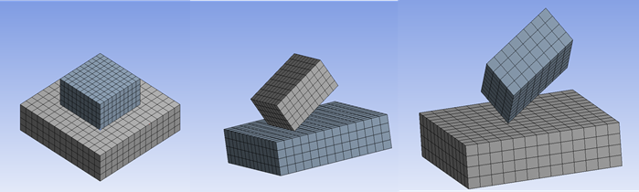
To illustrate the difference between the ORTHO and FORTHO options, consider the example of a flexible rectangular block meshed with contact elements which is pressed down on a rigid target surface on the global X-Z plane. Orthotropic friction can be defined as:
TB,FRIC,,,ORTHO     ! TBOPT = ORTHO
TBDATA,,0.2,0.001   ! MU1 = 0.2, MU2 = 0.001
or
TB,FRIC,,,FORTHO
TBDATA,,0.2,0.001
The friction coordinate system is parallel to the global coordinate system, with the two principal directions initially parallel to the global X and global Z directions.
First, the block slides in the +X direction and then slides back to the starting position. During this sliding motion, the block experiences a friction coefficient of 0.2 for both the ORTHO and FORTHO options.
Next, the block is rotated 90° and made to slide along the Z direction. For the ORTHO option, the block experiences the same friction coefficient of 0.2 in the Z direction since the friction coordinate system has also rotated with the block and contact elements. However, for the FORTHO option, the block experiences a friction coefficient of 0.001 in the Z direction after the rotation since the friction coordinate system is fixed.
The animations below show contour plots of frictional force experienced by the block when the ORTHO and FORTHO options are used. Note the almost zero frictional force after the rotation in the FORTHO case.

The program provides one extension of classical Coulomb friction: real
constant TAUMAX is maximum contact friction with units of stress. This maximum
contact friction stress can be introduced so that, regardless of the magnitude
of normal contact pressure, sliding will occur if the friction stress reaches
this value. You typically use TAUMAX when the contact pressure becomes very
large (such as in bulk metal forming processes). TAUMAX defaults to 1.0e20.
Empirical data is often the best source for TAUMAX. Its value may be close to
 , where σy is the yield stress of
the material being deformed.
, where σy is the yield stress of
the material being deformed.
You have an option to define TAUMAX as a function of primary variables by
using tabular input (that is, %tabname%). The
possible primary variables include time, temperature, initial contact detection
point location (at the beginning of solution), current contact pressure
(positive PRESSURE index values indicate compression, negative PRESSURE index
values indicate tension), and current geometric penetration (positive GAP index
values indicate penetration, negative GAP index values indicate an open gap).
For more information, see Defining Real Constants in Tabular Format.
The user subroutine USERCNPROP.F is also available for
defining TAUMAX. To use this subroutine, you must specify the table name
%_CNPROP% as the real constant value. For more information, see Defining Real Constants via a User Subroutine.
Another real constant used for the friction law is the cohesion, COHE (default COHE = 0), which has units of stress. It provides sliding resistance, even with zero normal pressure (see Figure 3.17: Sliding Contact Resistance).
Two other real constants, FACT and DC are involved in specifying static and dynamic friction coefficients, as described in the next section.
The coefficient of friction can depend on the relative velocity of the surfaces in contact. Typically, the static coefficient of friction is higher than the dynamic coefficient of friction.
The program provides the following exponential decay friction model:

where:
| μ = coefficient of friction. |
| MU = dynamic coefficient of friction. |
| FACT = ratio of static to dynamic coefficients of friction. It defaults to the minimum value of 1.0 |
| DC = decay coefficient, which has units of time/length. Therefore, time has some meaning in a static analysis. DC defaults to zero. When DC is zero, the equation is rewritten to be μ = MU for the case of sliding and μ = FACT*MU for the case of sticking. |
| Vrel = slip rate calculated by the program. |
For the isotropic friction model, MU is input using the MP command or the TB command as explained above. For orthotropic friction, MU is the equivalent coefficient of friction computed from MU1 and MU2 which are specified with TB command input:

Figure 3.18: Friction Decay shows the exponential decay curve where the static coefficient of friction is given by:


You can determine the decay coefficient if you know the static and dynamic coefficients of friction and at least one data point (μ1 ; Vrel1). The equation for friction decay can be rearranged to give:

If you do not specify a decay coefficient and FACT is greater than 1.0, the coefficient of friction will change suddenly from the static to the dynamic value as soon as contact reaches the sliding state. This behavior is not recommended because the discontinuity may lead to convergence difficulties.
In a static analysis, you can model steady-state frictional sliding between two flexible bodies or between a flexible and a rigid body with different velocities. In this case the sliding velocities no longer follow the nodal displacements, and they are predefined through the CMROTATE command. This command sets the velocities on the nodes of the element component as an initial condition at the start of a load step. The program determines the sliding direction based on the direction of the sliding velocities.
This feature is applicable to 3D contact (CONTA174, CONTA175) and is primarily used for generating sliding contact at frictional contact interfaces in a brake squeal analysis. In this case, the contact pair elements (either the contact elements or the target elements) on the brake rotor need to be included in the rotating element component (CM command) that is specified on the CMROTATE command. Ansys recommends that you include only the contact elements or only the target elements in the element component.
Velocities defined by CMROTATE will be ignored for the following contact definitions:
| Frictionless contact |
| Rough contact (KEYOPT(12) = 1) |
| Bonded contact (KEYOPT(12) = 3, 5, 6) |
| MPC contact (KEYOPT(2) = 2) |
Note: You should always verify the sliding direction when the velocities defined by CMROTATE are applied on nodes that are shared by more than one frictional contact pair. In this situation, you can redefine any contact elements that have a potentially incorrect sliding direction as frictionless contact.
The amplitude of the sliding velocity defined by CMROTATE will affect the solution when the friction coefficient is specified as a function of sliding velocity via the command TB,FRIC, or when static and dynamic friction is defined via the real constants FACT and DC.
In a complex eigenvalue extraction analysis using the QRDAMP or DAMP methods (see MODOPT), the effects of squeal damping will contribute to the damping matrix. The squeal damping can be identified as two parts: destabilizing damping and stabilizing damping.
You can activate destabilizing squeal damping by one of the following methods:
Define friction as a function of sliding velocity via the TB,FRIC command.
Define static/dynamic friction via real constants FACT and DC.
Define a constant friction-sliding velocity gradient via real constant FDMD in conjunction with KEYOPT(16) = 1.
Specify the destabilizing squeal damping coefficient directly (either a positive or negative value) in conjunction with KEYOPT(16) = 2.
When the destabilizing squeal damping is included by method (1) or (2), you can study its effects by using FDMD as a scaling factor (KEYOPT(16) = 0). FDMD defaults to 1.0. The program multiplies the internally calculated destabilizing damping by this factor.
You can specify a constant friction-sliding velocity gradient directly via FDMD by setting KEYOPT(16) = 1. The defined gradient has units of TIME/LENGTH and it is negative in general.
You can also specify the destabilizing squeal damping coefficient directly via FDMD by setting KEYOPT(16) = 2. The defined damping coefficient has units of MASS/(AREA*TIME) and it is negative in general. In a linear non-prestressed modal analysis, this is the only way to take the destabilizing squeal damping effects into account.
The stabilizing squeal damping is deactivated by default. To activate it, you must specify the scaling factor via the real constant FDMS. FDMS defaults to 0.0. The program multiplies the internally calculated stabilizing damping by this factor. By setting KEYOPT(16) = 1 or KEYOPT(16) = 2 you can specify the stabilizing squeal damping coefficient directly via FDMS. The defined damping coefficient has units of MASS/(AREA*TIME) and it is positive in general. In a linear non-prestressed modal analysis, this is the only way to take the stabilizing squeal damping effects into account.
If squeal damping is included in a brake squeal modal analysis that uses the QR Damp eigensolver (MODOPT,QRDAMP command), care should be taken not to generate a damping matrix with large values (coefficients) relative to the values of the stiffness matrix. The accuracy of the QRDAMP eigensolver is based on the assumption that the values in the damping matrix are at least an order of magnitude smaller than the stiffness matrix values. If large squeal damping matrix values are generated in conjunction with a QRDAMP modal solution, then the QRDAMP eigensolver could produce spurious zero modes, which can generally be ignored. In this case, the non-zero eigenvalues from the QRDAMP modal solution are still accurate. Ansys recommends that you use the DAMP eigensolver (MODOPT,DAMP) to check the final solution.
As a special case, when contact friction is used in a steady-state rolling analysis, the frictional stress calculation is changed to a viscous formulation. For details, see Contact Algorithm in the Theory Reference.
The following topics related to selecting the location of contact detection are available:
Contact detection points are located at the integration points of the contact elements which are interior to the element surface. The contact element is constrained against penetration into the target surface at its integration points. However, the target surface can, in principle, penetrate through into the contact surface, see Figure 3.19: Contact Detection Located at Gauss Point.
Surface-to-surface contact elements use Gauss integration points as a default, which generally provide more accurate results than the nodal detection scheme, which uses the nodes themselves as the integration points. The node-to-surface contact element, CONTA175, and the line-to-surface contact element, CONTA177, always use the nodal detection scheme.
The nodal detection algorithms require the smoothing of the contact surface (KEYOPT(4) = 1) or the smoothing of the target surface (KEYOPT(4) = 2), which is quite time consuming. You should use this option only to deal with corner, point-to-surface, or edge-to-surface contact (see Figure 3.20: Contact Detection Point Location at Nodal Point). KEYOPT(4) = 1 specifies that the contact normal be perpendicular to the contact surface. KEYOPT(4) = 2 specifies that the contact normal be perpendicular to the target surface. Use KEYOPT(4) = 2 when the target surface is smoother than the contact surface.
Be aware, however, that using nodes as the contact detection points can lead to other convergence difficulties, such as node slippage, where the node slips off the edge of the target surface, see Figure 3.21: Node Slippage Using Nodal Detection KEYOPT(4) = 1 or 2. In order to prevent node slippage, you can use real constant TOLS to extend the target surface when the default setting still cannot avoid the problem. For most point-to-surface contact problems, Ansys recommends using CONTA175. See Node-to-Surface Contact later in this guide.
Smoothing is required for nodal detection algorithms, and it is performed by averaging surface normals connected to the node. As a result, the variation of the surface normal is continuous over the surface, which leads to a better calculation of friction behavior and a better convergence.
Real constant TOLS is used to add a small tolerance that will internally extend the edge of the target surface when you define the contact detection at the nodal point (KEYOPT(4) = 1 or 2). TOLS is useful for problems where contact nodes are likely to lie on the edge of targets (as at symmetry planes or for models generated in a node-to-node contact pattern). In these situations, the contact node may repeatedly slip off the target surface and go completely out of contact, resulting in convergence difficulties from oscillations. Units for TOLS are percent (1.0 implies a 1.0% increase in the target edge length). A small value of TOLS will usually prevent this situation from occurring. The default value is 2 for both small deflection (NLGEOM,OFF) and large deflection (NLGEOM,ON).
Note: For Normal Lagrange formulation (KEYOPT(2)=3,4), with 3D higher-order contact elements (with midside nodes), use of surface projection-based contacts (KEYOPT(4)=3,4) is strongly recommended.
The definition of KEYOPT(4) in node-to-surface contact element CONTA175 is different. KEYOPT(4) = 1 for surface-to-surface contact is equivalent to KEYOPT(4) = 1 for node-to-surface contact. However, KEYOPT(4) = 2 for surface-to-surface contact is equivalent to KEYOPT(4) = 0 for node-to surface contact. See KEYOPT(4).
You can define the surface projection contact method by setting KEYOPT(4) = 3 or 4 for the surface-to-surface contact elements (CONTA172 and CONTA174) and the line-to-surface contact element (CONTA177):
KEYOPT(4) = 3 – Standard surface projection
KEYOPT(4) = 4 – Dual shape function projection
For CONTA172 and CONTA174, a unified contact detection approach is also available:
KEYOPT(4) = 5 – Unified approach which combines the standard surface projection with Gauss and the normal-to-target-surface nodal detection method
Standard Surface Projection and Dual Shape Function Projection Options (KEYOPT(4) = 3 or 4)
For the standard surface projection (KEYOPT(4) = 3) and dual shape function projection (KEYOPT(4) = 4) options, the contact detection remains at contact nodal points. These options enforce a contact constraint on an overlapping region of the contact and target surfaces (see Figure 3.22: Surface Projection Based Contact) rather than on individual contact nodes (KEYOPT(4) = 1, 2) or Gauss points (KEYOPT(4) = 0). The contact penetration/gap is computed over the overlapping region in an average sense. Advantages of the surface projection based method are:
In general, it provides more accurate contact tractions and stresses of underlying elements compared with other KEYOPT(4) settings.
The results are less sensitive to the designation of the contact and target surface.
It satisfies moment equilibrium when an offset exists between contact and target surfaces with friction.
Contact forces do not jump when contact nodes slide off the edge of target surfaces. The real constant TOLS is not used with this option.

There are certain disadvantages to using surface projection based contact, as follows:
This method is computationally more expensive since more nodes are included in each contact constraint condition, especially if 3D higher order contact/target elements are used in the model. This effect will be more obvious when a modal has a large percentage of contact/target elements, or when the target elements are much more refined than the contact elements.
When the target elements are extremely refined, the program may issue an error message stating that the data points for a particular node exceed the limit. To resolve this, you should switch to another contact detection option or flip the contact and target surfaces.
This method calculates the penetration/gap over the contacting area in an average sense. When a model has corner or edge contact, the averaged penetration/gap could be quite different than the real geometric penetration observed at contact nodes. In this situation, mesh refinement is usually required in order to achieve an accurate solution.
Comparison of the Standard Projection Option and the Dual Shape Function Option
Compared to the standard surface projection option (KEYOPT(4) = 3), the dual shape function projection option (KEYOPT(4) = 4) uses a special interpolation function for the discretization of contact traction. This option reduces dependent terms for each contact constraint. The resulting gap function and slip increments are closer to the local geometric gap/slip at contact nodes. It is more efficient in terms of solution performance and memory usage and generally remedies potential overconstraint due to MPC equations.
The dual shape function option is recommended for Lagrange multiplier contact (KEYOPT(2) = 3 or 4), MPC bonded contact (KEYOPT(2) = 2), and small sliding behavior (KEYOPT(18) = 1 or 2). For MPC bonded contact, the program internally switches to the dual shape function option if the standard projection option is defined.
Be aware that the dual shape function option is not as accurate as the standard projection option when the contact surface mesh is very coarse.
Unified Contact Detection Approach (KEYOPT(4) = 5)
Selecting the best contact detection is problem dependent and can have a significant impact on the solution. Each detection method has advantages and disadvantages:
For standard surface projection (KEYOPT(4) = 3) and dual shape function projection (KEYOPT(4) = 4), the penetration or gap at each contact node is an average value from the projected area. Thus, for corner and edge contact, the nodes on the corner or edge will penetrate the target surface which could result in large penetrations.
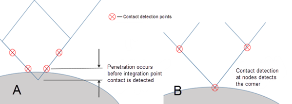
The same drawback applies to Gauss point detection (KEYOPT(4) = 0). If the contact surface has significant curvature or a corner, the contact surface can penetrate into the target surface (see A in the figure below).
Nodal point detection with normal to target (KEYOPT(4) = 2) is better suited for edge or corner contact (see B in the figure below). However, the contact node can easily drop off the edges of the target surface, causing a sudden jump in internal contact forces.
No detection method works best for all problems. One detection method may be obviously better for the early stage of the deformation, while another method may work better for the later stages.
To overcome this problem, the unified contact detection option (KEYOPT(4) = 5) combines three individual contact detection methods: Gauss point, nodal point with normal to target, and standard surface projection. This approach generally overcomes drawbacks of each individual method. The main advantages are:
More contact constraint points for the contact interface
Lower residual penetration
Less sensitivity to mesh sizing at the contact interface
Lower number of equilibrium iterations
Furthermore, the unified detection approach in conjunction with a symmetric contact definition works robustly for non-smoothing contact. Interference fit, press fit, snap fit, and snap-through are typical applications that can benefit from the unified contact approach.
The figure below shows a contact pair with mixed surfaces, edges, and corners under large deformations and displacements.
Keep in mind that the unified approach is the most expensive option. Use of additional features such as adaptive small sliding (KEYOPT(18) = 2) and contact pair-splitting logic (CNCHECK,DMP) often improve the performance.
Limitations for Surface Projection Based Contact (KEYOPT(4) = 3, 4, or 5)
The surface projection contact method currently does not support the following:
Thermal contact modeled via a “free thermal surface” definition.
Pore fluid flow modeled by quadratic contact/target elements (with midside nodes).
Rigid surfaces defined by primitive target segments. (This type of rigid surface is supported for the unified approach (KEYOPT(4) = 5) when only the Guass and nodal detection methods are used.)
3D contact/target elements with partially dropped midside nodes (dropping all midside nodes is supported).
The unified approach (KEYOPT(4) = 5) does not support:
The MPC formulation (KEYOPT(2) = 2).
Nonlinear mesh adaptivity (NLADAPTIVE)
The following sliding behavior topics are available:
Three different sliding behavior options are available: finite sliding (default), small sliding, and adaptive small sliding. The sliding behavior you choose will have an influence on solution robustness, performance, and accuracy. Select the appropriate sliding behavior based on the relative motion of the contact interfaces in your model.
The finite-sliding option is used by default (KEYOPT(18) = 0). This option allows for arbitrary separation, sliding, and rotation of the contact interfaces. In general, each contact detection point can interact with different target elements, depending on the contact status (open, closed, or sliding). The program re-forms nodal connectivity of the contact element based on the current configuration at each equilibrium iteration. The finite-sliding logic is computationally expensive, but guarantees solution accuracy.
Activate the small-sliding option (KEYOPT(18) = 1) when the contact interface will have relatively-small sliding motion (less than 20% of the contact length) during the entire analysis. For large deflection analysis, this option still permits arbitrary large rotation.
For small sliding, each contact detection point always interacts with the same target element, which is determined from the initial configuration. The nodal connectivity of the contact element remains unchanged throughout the analysis. Contact searching is performed only once in the beginning of the analysis, which is cost-effective.
The small-sliding logic also improves solution robustness. It can easily solve certain complex contact models for which the finite-sliding logic would have difficulties or find no solution. This is especially true for models having a bad quality geometry or mesh and non-smooth contact interfaces. (See this white paper for more discussion of this behavior.)
The small-sliding logic can cause nonphysical results if the relative sliding motion does not remain small. Therefore, if you choose this option it is your responsibility to ensure that the small-sliding assumption is not violated. Use the NLHIST or NLDIAG command to monitor the number of contact points having too much sliding (that is, the SLID value is greater than 50% of the contact length or 50% of the associated target element length).
Use the finite-sliding option if you are not absolutely sure that the small-sliding logic is appropriate.
Use the small-sliding option with great caution for the following cases:
The EKILL command applied to target elements of contact pairs using the projection-based contact option (KEYOPT(4) = 3, 4, or 5)
A general contact definition
Activate the adaptive small-sliding option (KEYOPT(18) = 2) when the contact interface will have relatively-small sliding motion (less than 20% of the contact length) during each sub-step of the analysis. The contact interface can undergo either small sliding or finite sliding within each substep based on the contact status at the beginning of the substep. If the contact status is closed at the beginning of a substep, small sliding is used during that substep.
For this option, each contact detection point interacts with the same target element, which is determined from the beginning configuration of each substep. The nodal connectivity of the contact element remains unchanged during the substep.
The adaptive small-sliding logic often improves robustness compared to the finite sliding logic and can also improve solution accuracy compared to the small sliding logic. It can handle situations when contact pairs are initially in far-field and then come into contact.
The adaptive small-sliding logic may cause nonphysical results if the relative sliding motion does not remain small within a substep. To avoid this, activate additional time step control (KEYOPT(7) > 0) so that bisection is performed if a large sliding distance is detected within a substep.
To ensure solution accuracy, use the NLHIST or NLDIAG command to monitor the number of contact points having too much sliding (that is, the SLMX value is greater than 50% of the contact length or 50% of the associated target element length).
The following topics related to adjusting initial contact conditions are available:
Rigid body motion is usually not a problem in dynamic analyses. However, in static analyses, rigid body motion occurs when a body is not sufficiently restrained. "Zero or negative pivot" warning messages and impractical, excessively large displacements indicate unconstrained motion in a static analysis.
In simulations where rigid body motions are constrained only by the presence of contact, you must ensure that the contact pairs are in contact in the initial geometry. In other words, you want to build your model so that the contact pairs are "just touching." However, you can encounter various problems in doing so:
Rigid body profiles are often complicated, making it difficult to determine where the first point of contact might occur.
Small gaps between element meshes on both sides of the element pair can be introduced by numerical round-off, even if the solid model is built in an initially-contacting state.
Small gaps can exist between the integration points of the contact elements and target surface elements.
For surface projection based contact, a numerical gap distance can exist even though geometric penetration is observed at a contact node. This can occur because the numerical distance is obtained over the overlapping area in an average sense.
For the same reasons, too much initial penetration between target and contact surfaces can occur. In such cases, the contact elements may overestimate the contact forces, resulting in nonconvergence or in breaking-away of the components in contact.
The definition of initial contact is perhaps the most important aspect of building a contact analysis model. Therefore, you should always issue the CNCHECK command before starting the solution to verify the initial contact status. You may find that you need to adjust the initial contact conditions. The program offers several ways to adjust the initial contact conditions of a contact pair.
Note: When contact or target elements are deactivated (EKILL command) in the first load step, the program might not adjust the initial contact conditions correctly. Therefore, you should not deactivate contact or target elements at the beginning of the analysis if you wish to make initial contact adjustments.
The following techniques can be performed independently or in combinations of one or more at the beginning of the analysis. They are intended to eliminate small gaps or penetrations caused by numerical round-off due to mesh generation. They are not intended to correct gross errors in either the mesh or in the geometric data.
Use real constant CNOF to specify a contact surface offset.
Specify a positive value to offset the entire contact surface toward the target surface. Use a negative value to offset the contact surface away from the target surface.
Note: If user-defined values are input for both CNOF and PINB, you must ensure that PINB is greater than CNOF. Otherwise, CNOF will be ignored. However, if a user-defined CNOF is input and the PINB value is left at its default value, the PINB value will be adjusted so that it is larger than the CNOF value, as described in Using PINB.
Note: For the CONTA177 line-to-surface element, CNOF can be used to model thickness of the underlying beam elements. Input half of the beam thickness for CNOF to properly model the thickness effects. See Accounting for Thickness Effect (KEYOPT(11)) for more information.
The program can automatically provide the CNOF value to either just close the gap or reduce initial penetration. Set KEYOPT(5) as follows:
1: Closes the gap2: Reduces initial penetration3: Either closes the gap or reduces initial penetrationTabular input can also be used to define CNOF. The tabular input can be defined as a function of time and/or initial contact detection point location (at the beginning of solution) in global or local coordinates. For more information, see Defining Real Constants in Tabular Format.
As an example of when tabular input may be useful, consider the case of a CAD geometry based on nominal values. The geometry may lack a slight curvature variation that is important for analysis purposes. Moving nodes to the actual positions can be a tedious process, yet using the original geometry and neglecting the slight variation in curvature will result in a different contacting area. Consequently, use of CNOF as a function of location allows you to easily include curvature that varies with location without having to modify the original CAD geometry.
The user subroutine
USERCNPROP.Fis also available for defining CNOF. To use this subroutine, you must specify the table name %_CNPROP% as the real constant value. For more information, see Defining Real Constants via a User Subroutine.Use the real constant ICONT to specify a small initial contact closure. This is the depth of an "adjustment band" around the target surface. A positive value for ICONT indicates a scaling factor relative to the depth of the underlying elements. A negative value indicates an absolute contact closure value. The value of ICONT defaults to zero if KEYOPT(5) = 0, 1, 2, or 3. If KEYOPT(5) = 4, the program provides a small (but meaningful) value for ICONT according to the geometric dimensions, and prints a warning message stating what value was assigned. Any contact detection points that fall within this adjustment band are internally shifted to be on the target surface (see Figure 3.25: Contact Surface Adjustment With ICONT(a)). Only a very small correction is suggested. Otherwise, severe discontinuity may occur (see Figure (b)).
The difference between CNOF and ICONT is that the former shifts the entire contact surface with the distance value CNOF, the latter moves all initially open contact points which are inside of adjustment band ICONT onto the target surface.
Set KEYOPT(9) to adjust initial penetration or gap. See Figure 3.26: Ignoring Initial Penetration, KEYOPT(9) = 1.
True initial penetration includes two parts:
Penetration or gap due to geometry
Penetration or gap due to user-defined contact surface offset (CNOF).
See Figure 3.27: Components of True Penetration.
Keep in mind that the effects of KEYOPT(9) are dependent on settings for other KEYOPTs. The indicated initial gap effect is considered only if KEYOPT(12) = 4 or 5 (no separation always or bonded always).
KEYOPT(9) offers the following settings for adjusting initial penetration or gap:
To include initial penetration or gap from both geometry and contact surface offset, set KEYOPT(9) = 0. This is the default.
To ignore initial penetration or gap from both geometry and contact surface offset, set KEYOPT(9) = 1.
To include the defined contact surface offset (CNOF) but ignore the initial penetration or gap due to geometry, set KEYOPT(9) = 3.
Set KEYOPT(9) = 5 to include the defined contact surface offset (CNOF) but ignore the initial penetration due to geometry. Even when KEYOPT(12) is not set to 4 or 5, this setting for KEYOPT(9) will also ignore the initial force in open-gap springs as long as contact is detected within the pinball region.
For problems such as an interference fit, over-penetration is expected. These problems often have convergence difficulties if the initial penetration is step-applied in the first load step. You may overcome convergence difficulties by ramping the initial penetration over the first load step. See Figure 3.28: Ramping Initial Interference. The following KEYOPT(9) settings provide ramping capabilities:
To ramp the total initial penetration or gap (CNOF + the offset due to geometry), set KEYOPT(9) = 2.
To ramp the defined contact surface penetration or gap (CNOF), but ignore the penetration or gap due to geometry, set KEYOPT(9) = 4.
Set KEYOPT(9) = 6 to ramp the defined contact offset (CNOF) but ignore the initial penetration due to geometry. Even when KEYOPT(12) is not set to 4 or 5, this setting for KEYOPT(9) will also ignore the initial force in open-gap springs as long as contact is detected within the pinball region.
For the above KEYOPT(9) settings, you should not specify any external loads in the first load step. In addition, make sure that the pinball region is big enough to capture the initial interference.
For KEYOPT(9) = 0, 1, 3, or 5, the default pinball (PINB) value is half that of the KEYOPT(9) settings that include ramped effects (KEYOPT(9) = 2, 4, or 6). The default PINB value may differ from what is described here if CNOF is input. See Defining the Pinball Region (PINB) for more information.

You can use the above techniques in conjunction with each other. For example, you may wish to set a very precise initial penetration or gap, but the initial coordinates of the finite element nodes may not be able to provide sufficient precision. To accomplish this, you could:
Use CNOF to specify a penetration (positive value) or gap (negative value).
Use KEYOPT(9) = 5 to resolve the initial penetration in the first substep (or KEYOPT(9) = 6 to gradually resolve the initial penetration).
The program provides a printout (in the output window or file or via the CNCHECK) of the model's initial contact state for each target surface at the beginning of the analysis. This information is helpful for determining the maximum penetration or minimum gap for each target surface.
If no contact is detected for a specific target surface, the program issues a warning. This occurs when the target surface is far from contact (that is, outside of the pinball region), or when the contact/target elements have been killed.
See Positive and Negative Real Constants for more information on these real constants.
You can model an interference fit to simulate penetration between parts in the initial geometry configuration. In general, the initial penetrations associated with an interference fit are much larger than in standard contact assemblies. These large initial penetrations cannot be resolved in one substep (that is, step-applied).
Mechanical APDL offers several approaches that solve the large initial penetrations gradually over a load step with multiple substeps. These methods enable you to control the number of substeps or time increments to accomplish the interference fit. Once the interference fit is resolved, you can continue the analysis in a new load step.
There are three different methods to resolve large penetrations for an interference fit:
1. Contact surface offset (CNOF) as a function of time via tabular input — Use tabular input to specify a table in which the magnitude of CNOF is ramped down from the possible maximum values of interference to zero over time. Be sure to input negative values in the defined table to offset the contact surface away from the target surface. In this way, the program will treat the initial contact interface as just touching at the beginning of the load step and push the surfaces apart gradually until the end of load step. This method is recommended for situations in which the interference is nearly uniform across the interface and CNOF is a function of time. It is not recommended when CNOF is a function of both time and location. For this method you do not need to set a ramping option (KEYOPT(9) = 2 or 4).
2. Automatically ramp down the initial penetration — Set KEYOPT(9) = 2 or 4 to activate this method. There are two options within this method:
(a) Ramping the initial penetration down to zero over time along the true contact normal direction. This is the default option, which is appropriate for most applications. However, when the contact and/or target surfaces are not smooth, the contact normal direction varies across the interface, which may lead to locking of the press fit.
(b) Ramping the initial penetration down to zero over time along a user-defined shift direction. Use this option to remedy possible locking issues that could occur with the (a) option. The user-defined shift direction is defined via the SECTYPE and SECDATA commands. In certain applications, such as contact simulations of threaded connectors, convergence behavior improves when a user-defined contact surface normal is used instead of the default contact normal. Since the user-defined contact surface normal is defined only on the contact elements, the “Normal to target surface” option is recommended (KEYOPT(4) = 2 for CONTA172 and CONTA174, KEYOPT(4) = 0 for CONTA175). This option is not available for CONTA177. For details, see User-Defined Contact Surface Normal.
By default, this ramping method is active only within the first load step for both the (a) and (b) options. However, you may have a situation where there are multiple interference fits that you want to model sequentially (that is, the interference present in each contact pair will be resolved in different load steps). You can define the load step number in which the ramping option will take place for a given contact pair by using real constant STRM. For example, you may want to perform a different loading in load step 1, then resolve an interference fit in load step 2 for one contact pair, and finally resolve an interference fit in load step 3 for another contact pair. To accomplish this, you would set STRM = 2 for the first contact pair and set STRM = 3 for the second contact pair. Note that contact is still active prior to the load step specified by the STRM real constant.
3. Automatically ramp up the contact stiffness — Set KEYOPT(9) = 2 or 4 and define real constants STRM and/or TEND to activate this method. The program automatically ramps the normal and tangential contact stiffness as well as the friction coefficient (that is, FKN, FKT, MU) from near-zero to actual values. You control when the ramping is active—in a particular time step or over a specified time period—by setting the real constants in one of two ways:
(a) Use STRM (a negative integer) to define the load step number and leave TEND undefined. The program automatically ramps FKN, FKT, and MU from near-zero to actual values within the defined load step. For example, you may want to perform a different loading in load step 1, then resolve an interference fit in load step 2 for one contact pair, and finally resolve an interference fit in load step 3 for another contact pair. To accomplish this, set STRM = -2 for the first contact pair and set STRM = -3 for the second contact pair.
When STRM is set to -1 to indicate the first load step and the initial contact status is open or the initial penetration is smaller than the penetration tolerance, the program turns off the stiffness ramping logic by resetting STRM to 0. This is done to improve solution convergence.
(b) Use STRM to define the starting time of the ramping and TEND (no default) to define the ending time. STRM defaults to 0 (beginning of the analysis). The program automatically ramps FKN, FKT, and MU from near-zero to actual values within the period of the starting time (STRM) and the ending time (TEND). The time period can be defined within one load step or across several load steps.
For both the (a) and (b) options of this method, contact does not need to be engaged or well established in the initial configuration. A very tiny contact stiffness is used internally prior to the ramping load step or time period.
For methods 1 and 2, you need to specify the pinball radius (real constant PINB) to be larger than the maximum initial penetration of the entire contact pair so that the contact is still well engaged in the beginning of the analysis. The initial interference fit is usually solved under frictionless conditions. You can explicitly define zero or near-zero friction in the beginning of the analysis and apply the friction right after the interference fit is fully resolved.
For methods 2 and 3, you must set KEYOPT(9) = 2 or 4 to activate ramping of the penetration. Method 3 does not require a large pinball radius to capture the initial contact in the beginning of the analysis. However, it still requires a large enough pinball radius during the load step or time period for resolving the interference.
You can adjust the initial contact status in order to close the gap by doing one of the following:
| (a) Define an initial contact adjustment via real constant ICONT. (ICONT may change the shape of the contact detection surface.) |
| (b) Define a contact offset via real constant CNOF. (CNOF does not change the shape of the contact detection surface.) |
| (c) Ignore the penetration by setting KEYOPT(9) = 1. (KEYOPT(9) = 1 does change the shape of the contact detection surface.) |
However, these adjustment methods do not truly change the physical locations of contact nodes. Rather, the contact detection locations are adjusted.
The initial adjustment due to (a) is applied only once in the beginning of the contact analysis, where each contact detection point within the ICONT range is made to be in initial contact with the target surface. The contact adjustments due to (b) and (c) offset the entire contact detection surface to close any gap that is present. In doing so, methods (b) and (c) introduce a "rigid region" between the contact and target surfaces during the entire analysis, which can cause a certain amount of residual force if a large rotation appears at the contact surface. This problem can be alleviated by issuing the CNCHECK,ADJUST or CNCHECK,MORPH command.
CNCHECK,ADJUST physically moves contact nodes toward the target surface while leaving the rest of the model untouched. Similarly, CNCHECK,MORPH moves contact nodes toward the target surface, but also morphs the underlying solid element mesh to improve the mesh quality that was distorted due to movement of the contact nodes. (If you want to adjust the physical location of the model, refer to Physically Moving the Target Body Toward the Contact Surface.)
Both CNCHECK,ADJUST and CNCHECK,MORPH move the contact nodes to the target surface under the following circumstances:
If the default adjustment behavior is not desired, you can define further controls using the following additional fields on the CNCHECK,ADJUST or CNCHECK,MORPH command:
CGAP- Control parameter for opening gap. When this value is specified, an opening gap closes if the absolute value of the gap is smaller thanCGAP.CGAPdefaults to 0.25*PINB (where PINB is the pinball radius) for bonded and no-separation contact. Otherwise, it defaults to the value of real constant ICONT.CPEN- Control parameter for initial penetration. When this value is specified, initial penetration closes if the absolute value of the penetration is smaller thanCPEN.CPENdefaults to 0.25*PINB (where PINB is the pinball radius) for any type of interface behavior (either bonded or standard contact).IOFF- Control parameter for initial adjustment. Input a positive value to adjust the contact nodes toward the target surface with a constant interference distance equal toIOFF. Input a negative value to adjust the contact node toward the target surface with a uniform gap distance equal to the absolute value ofIOFF.
By default, the CGAP and
CPEN adjustments modify initial node positions such
that the contact surface and the target surface are “just-touching”
(with zero penetration/gap). Alternatively, you can specify
IOFF to adjust nodal positions such that a constant
offset (equal to IOFF) exists between the contact surface
and target surface initially. The adjustments will take place only for regions that
are inside the adjusted zone as discussed above. You should always carefully review
the adjustment since mesh distortion may occur if the adjustment is too large to
achieve the specified control parameters.
If KEYOPT(4) = 0 (contact detection on Gauss point), the program automatically sets KEYOPT(4) = 1 (contact detection on nodal point) for CONTA172 and CONTA174 and sets KEYOPT(9) = 1 for selected contact elements. It then sets KEYOPT(4) and KEYOPT(9) back to their previous settings after the adjustment. In this case, the penetration/gap calculation using KEYOPT(4) = 0 might be different than the CNCHECK results which are calculated using KOYOPT(4) = 1 as the detection method has changed. If these differences are not desirable, use a consistent nodal detection method (KEYOPT(4) = 1, 2, 3, 4, or 5) for both the CNCHECK adjustment and the subsequent solution.
If you do not want all contact surfaces to be adjusted, you
can selectively identify the surfaces to move by specifying real constant IDs
(RID1, RID2,
RINC) on the CNCHECK command.
Using Tabular Input for
RID1
To avoid issuing multiple CNCHECK
commands, the RID1 argument can accept tabular input in
the form of a 2D array parameter. Create the array parameter using these
guidelines:
Real ID number is entered in the first column. Ascending order is preferred but not required. See Example 3.2: Simple Tabular Input for
RID1.The 2nd to 4th columns are
CGAP,CPENandIOFFvalues, as needed.The input format is %
tablename%, wheretablenameis a user-specified name.If tabular input is defined, the following CNCHECK command arguments are ignored:
RID2,RINC,Val1,Val2,Val3.If there is conflict in the table, the program uses the last valid input.
You can specify a negative row value to define a range of real IDs having the same
CGAP,CPENandIOFFvalues, as follows:If the real ID in the ith row (RIDrow i) has a negative value (RIDrow i = -n), the program interprets the range of real IDs as RIDrow i-1 to RID
n. All real IDs in this range are assigned the sameCGAP,CPENandIOFFvalues as RIDrow i-1. See Example 3.3: Tabular Input That Includes a Negative Real ID Value.
Example 3.2: Simple Tabular Input for RID1
*dim,cnchtable1,array,3,4         ! Define the an array parameter for tabular input
cnchtable1(1,1) = 4,   5,   3     ! Real IDs can be in arbitrary order
cnchtable1(1,2) = 0,   0, 0.1     ! CGAP
cnchtable1(1,3) = 1,   0,   0     ! CPEN
cnchtable1(1,4) = 0, -.1,   0     ! IOFF
cncheck,morph,%cnchtable1%
Example 3.3: Tabular Input That Includes a Negative Real ID Value
*dim,cnchtable2,array,3,4
cnchtable2(1,1) =   7,   3,  -5     ! Real ID = -5 means RID3, RID4, RID5 all have values assigned to RID3
cnchtable2(1,2) =   0, 0.1,   0     ! CGAP
cnchtable2(1,3) = 0.1,   0,   0     ! CPEN
cnchtable2(1,4) =   0,   0,   0     ! IOFF
cncheck,morph,%cnchtable2%
When the cnchtable2 array is input on the CNCHECK command, the program interprets it as:
| Real ID |
CGAP
|
CPEN
|
IOFF
|
| 7 | 0 | 0.1 | 0 |
| 3 | 0.1 | 0 | 0 |
| 4 | 0.1 | 0 | 0 |
| 5 | 0.1 | 0 | 0 |
Use the CNCHECK,ADJUST command when the gap or penetration to be adjusted is small enough that the movement of nodes will not cause significant mesh distortions. After the CNCHECK,ADJUST command is issued, the coordinates of the nodes that have been moved are modified as shown in Figure 3.29: Effect of Moving Contact Nodes via the ADJUST Option. You can change other contact related settings in PREP7 (for example, set KEYOPT(4) = 0 to use the Gauss detection option) and save the Jobname.db file. Issuing the SAVE command before issuing the CNCHECK,ADJUST command is recommended in order to resume the Jobname.db file with the original contact configuration.
The initial adjustment resulting from CNCHECK,ADJUST is converted to structural displacement values (UX, UY, UZ) and stored in a results file named Jobname.rcn. You can use this file to plot or list nodal adjustment vectors or create a contour plot of the adjustment magnitudes via the displacements (see Reviewing Results in POST1 for more information).
Sometimes, the gap or penetration between the contact and target surfaces is so large that moving the contact nodes to the target surface can result in significant mesh distortions. In this case, CNCHECK,MORPH should be used instead of CNCHECK,ADJUST to close gaps or reduce penetration.
When CNCHECK,MORPH is issued, the contact nodes are first moved toward the target (similar to he ADJUST option), then the underlying solid element mesh is morphed to improve the mesh quality. Figure 3.30: Comparison of the MORPH and ADJUST Options shows a case similar to that shown in Figure 3.29: Effect of Moving Contact Nodes via the ADJUST Option, but with a larger gap. This figure demonstrates that the MORPH option improves the mesh quality while moving the contact nodes to close the gap. CNCHECK,ADJUST (on the right) stretches the first layer of solid elements attached to the contact elements, while CNCHECK,MORPH (middle figure) results in a uniform mesh.
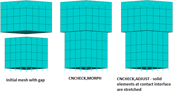
As shown in Figure 3.31: Effect of Boundary Conditions on the Morph Option, the final results can be different depending on whether or not you remove displacement constraints before issuing CNCHECK,MORPH. If CNCHECK,MORPH is issued with all constraints in place, the contact nodes are moved and the mesh is morphed to improve mesh quality. However, if CNCHECK,MORPH is issued after removing all displacement constraints, then the lower block is rigidly moved to touch the target surface.
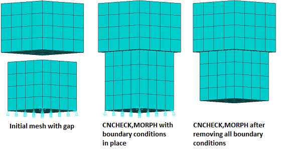
By default, all of the contact and target nodes are constrained during the
morphing process. Therefore, any of those nodes that did not move to close the
gap or penetration will likewise not move during the morphing process. To
circumvent this and allow boundary nodes attached to contact elements to move,
CNCHECK,MORPH unselects the far-field contact elements
(similar to CNCHECK,UNSELECT) before morphing the mesh. You
can further adjust the boundary node movements by setting
TRlevel = AGGRE on the
CNCHECK,MORPH command to automatically unselect additional
contact elements, therefore allowing movement of the boundary nodes attached to
them during morphing.
You can override the automatic unselect logic by manually unselecting the contact and target elements whose nodes you want to allow to move and applying displacement constraints on the nodes you want to prevent from moving. The manually unselected elements should be reselected after the morphing and before the actual solution.
Assumptions and Restrictions for CNCHECK,MORPH
CNCHECK,MORPH only supports solid elements. For other elements (shells, beams, links, and so on), CNCHECK,MORPH works like CNCHECK,ADJUST in that it will only move the contact nodes and will not morph the mesh.
CNCHECK,MORPH does not work with symmetric contact. If symmetric contact is desired, use auto-asymmetric contact (KEYOPT(8) = 2 or 3) during the adjustment phase. Once the mesh is adjusted, change the contact back to symmetric contact.
When used with a general contact definition, you must input section IDs (not real constant IDs) on the CNCHECK,MORPH command to identify surfaces that are to be adjusted. It is recommended that you always input specific section IDs since all surfaces in a general contact definition have contact elements overlaid on them. If specific section IDs are not specified, all contact surfaces will be considered and all boundary nodes will be fixed during morphing, which can result in a distorted mesh after morphing.
While the CNCHECK,ADJUST and CNCHECK,MORPH options move the contact surface to adjust the geometry in a relatively short distance, the CNCHECK,TADJUST option moves the entire target body to engage with the contact surface. The target body undergoes rigid body motion. Therefore, you mainly use TADJUST to establish contact between two bodies when there is a large gap. You can also use it for cases where ADJUST and MORPH would cause mesh distortion.
For flexible-to-flexible contact, this technique moves the entire target surface and the entire deformable body attached to the target surface. Make sure there are no other contact or target surfaces connected to the deformable body.
You can specify an upper and lower limit of initial allowable penetration
(PMAX and PMIN) on the
CNCHECK command. When PMAX or
PMIN is specified, the program brings the target
surface into a state of initial contact at the beginning of the analysis (see Figure 3.32: Target Surface Adjustment (PMAX,
PMIN)). If the initial penetration is larger than
PMAX, the program adjusts the target surface to
reduce penetration. If the initial penetration is smaller than
PMIN (and within the pinball region), the program
adjusts the target surface to ensure initial contact. Initial adjustment for contact
status is performed only in translational modes.
This initial contact adjustment can be performed for a rigid target surface that has either prescribed loads or displacements. A target surface that has no boundary conditions specified may also be adjusted.
When all the target surface nodes have a prescribed value of zero, the initial
adjustment using PMAX and PMIN
is not supported.
The program treats applicable degrees of freedom for target surface nodes independently.
For example, if you specify the UX degree of freedom to be zero, then no initial adjustment
is possible along the X direction. However, the PMAX and
PMIN options will still be activated in the Y and Z directions.
This is demonstrated in the below figures. When the target surface has no constraints,
CNCHECK,TADJUST moves the target body in the closest point-projection
direction to establish penetration. See Figure 3.33: Target Body Without Constraints - Before and After TADJUST. If the target
body is constrained in the X direction, the CNCHECK,TADJUST command can
only move the target body in the Y direction to establish penetration. See Figure 3.34: Target Body With Constraints - Before and After TADJUST.
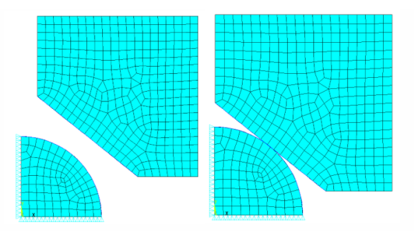
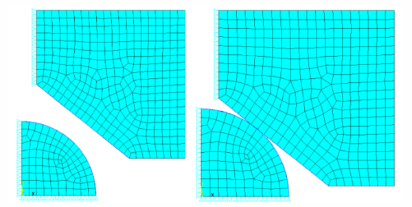
The initial status adjustment is an iterative process, with a maximum of 20
iterations. If the target surface cannot be brought into an acceptable penetration
range (PMIN to PMAX), the
analysis proceeds with the original geometry. In this case, the program issues a
warning message and you may need to manually adjust the initial geometry.
There can be scenarios for which the initial contact adjustment fails. In Figure 3.35: Example of Initial Adjustment Failure, the UY degree of freedom for the target has been restrained, and the only possible adjustment for initial contact is in the X direction. However, in this problem any movement of the rigid target surface in the X direction will not establish initial contact.
Using Tabular Input for
RID1
Like the ADJUST and MORPH options, the TADJUST option of CNCHECK
supports tabular input for the RID1 argument in the form of a 2D
array parameter. The first column contains real IDs. The second and third columns are
PMAX and PMIN, respectively.
If you have multiple contact pairs that need to be adjusted, the order of the CNCHECK operations can result in different geometries. Keep this in mind when creating tabular input.
As an example, consider the initial geometry (a) in the figure below, which has two contact pairs. Real ID 2 represents contact between the bottom and middle, and real ID 3 represents contact between the middle and top. Defining tabular input via the following command would result in geometry (b).
*dim,tadjtable,array,2,2
tadjtable(1,1)=3,2
tadjtable(1,2)=-0.002,-0.002
cnch,tadj,%tadjtable%
The program establishes contact in ascending real ID order: first 2, then 3. When the pair identified by real ID 3 is in contact, the pair identified by real ID 2 loses contact.
To resolve this, issue multiple CNCHECK,TADJUST commands instead of using tabular input. The input below results in the desired geometry (c).
CNCH,TADJ,3,, , , ,-0.002,
CNCH,TADJ,2,, , , ,-0.002,
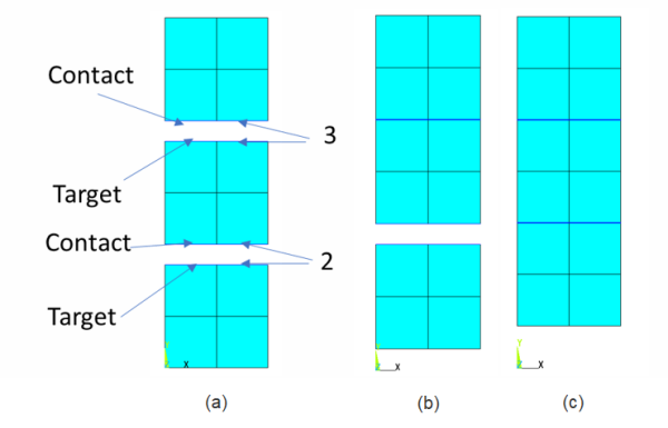
Limitation for CNCHECK,TADJUST
The CNCHECK,TADJUST option does not support the following:
Symmetric contact. As a workaround, unselect one pair of the symmetric contact pairs, then do the target body adjustment.
Two target surfaces on the same target body.
A target body constrained by a pilot node.
Beam-to-beam contact (CONTA177) in a crossing beam formation.
Comparison of TADJUST, ADJUST, and MORPH Options
The following table compares the three methods for adjusting contact surfaces.
| ADJUST | MORPH | TADJUST | |
| Surface to move | Contact | Contact | Target |
| Mesh morphing | No | Yes | No |
| Direction of move | Normal to contact surface | Normal to contact surface | Rigid body motion in non-constraint directions using shortest distance |
| Boundary condition restriction | Yes | Yes | Yes |
| Support for symmetric contact | Yes | Yes | No |
The following topics related to determining contact status and the pinball region are available:
The position and motion of a contact element relative to its associated target surface determines the contact element status. The program monitors each contact element and assigns a status:
STAT = 0 Open far-field contact (open and not near contact)
STAT = 1 Open near-field contact
STAT = 2 Sliding contact
STAT = 3 Sticking contact
A contact element is considered to be in near-field contact when its integration points (Gauss points or nodal points) are within a code-calculated (or user-defined) distance to the corresponding target surface. This distance is referred to as the pinball region. The pinball region is a circle (in 2D) or a sphere (in 3D) centered about the Gauss point.
Use real constant PINB to specify a scaling factor (positive value for PINB when using command input) or absolute value (negative value for PINB when using command input) for the pinball region. You can specify PINB to have any value.
By default, the program defines the pinball region as a circle for 2D or a sphere for 3D of radius 2*depth (if rigid-to-flexible contact) or 1*depth (if flexible-to-flexible contact) of the underlying element. See the discussion of element depth in Positive and Negative Real Constant Values. For the no-separation (KEYOPT(12) = 4), bonded-always (KEYOPT(12) = 5), and bonded-initial (KEYOPT(12) = 6) options, the PINB default is different than described here. See Selecting Surface Interaction Models for more information.)
If you input a value for real constant CNOF (contact surface offset) and the default PINB value is less than the absolute value of CNOF, the default for PINB will be set to the absolute value of (1.1*CNOF).
The computational cost of searching for contact depends on the size of the pinball region. Far-field contact (open and not near contact) element calculations are simple and add little computational demands. The near-field calculations (for contact elements that are nearly or actually in contact) are slower and more complex. The most complex calculations occur once the elements are in actual contact.
Setting a proper pinball region is useful to overcome spurious contact definitions if the target surface has several convex regions. However, the default setting should be appropriate for most contact problems.
For the purpose of trouble-shooting, note that the program uses a slightly larger pinball radius when reporting initial contact information (via the CNCHECK,DETAIL command or the Mechanical Contact Tool) than is actually used in the solution. This can help you to identify potentially missing or spurious contact.
The program warns you when there is an abrupt change in status (for example, from far-field to closed) during a contact analysis. This may indicate that the substep increment is too large, or possibly (but not likely) that the pinball value (PINB) is too small.
For more information about the PINB real constant, see Positive and Negative Real Constants.
In some cases of self contact, the program may erroneously assume contact between a contact and target surface that are in very close geometrical position as shown below.
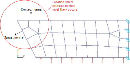
The program alerts you when it first detects spurious contact in each load step. If the program encounters such contact on the first load step, you'll see the following error message:
Contact element x has too much penetration related to target element y. We
assume it (may be more elements) is spurious contact.
If the program encounters an abrupt change in contact that it classifies as spurious contact, you'll see the following message:
Contact element x status changed abruptly with target element y. We assume
it (may be more elements) is spurious contact.
The program issues such messages only once per load step. It does not notify you of additional cases of spurious contact that were ignored during the load step.
The following topics related to selecting surface interaction models are available:
The surface-to-surface contact elements support normal unilateral contact models as well as other mechanical surface interaction models.
As an alternative to the program-supplied contact interactions, you can define
your own interfacial model with the USERINTER subroutine
(see User-Defined Subroutines for Contact Interfacial Behaviors).
Use KEYOPT(12) to model different contact surface behaviors.
KEYOPT(12) = 0 models standard unilateral contact. That is, normal pressure equals zero if separation occurs.
KEYOPT(12) = 1 models perfectly rough frictional contact where there is no sliding. This case corresponds to an infinite friction coefficient and ignores the material property MU.
KEYOPT(12) = 2 models no separation contact, in which the target and contact surfaces are tied (although sliding is permitted) for the remainder of the analysis once contact is established.
KEYOPT(12) = 3 models "bonded" contact, in which the target and contact surfaces are bonded in all directions (once contact is established) for the remainder of the analysis.
KEYOPT(12) = 4 models no separation contact, in which contact detection points that are either initially inside the pinball region or that once involve contact always attach to the target surface along the normal direction to the contact surface (sliding is permitted).
KEYOPT(12) = 5 models bonded contact, in which contact detection points that are either initially inside the pinball region or that once involve contact always attach to the target surface along the normal and tangent directions to the contact surface (fully bonded).
KEYOPT(12) = 6 models bonded contact, in which the contact detection points that are initially in a closed state will remain attached to the target surface and the contact detection points that are initially in an open state will remain open throughout the analysis.
For all types of bonded contact (KEYOPT(12) = 2, 3, 4, 5, and 6), separation of contact can be modeled using the debonding feature. For more information, see Debonding.
For the no-separation option (KEYOPT(12) = 4), the bonded-always option (KEYOPT(12) = 5), and bonded-initial option (KEYOPT(12) = 6 ) a relatively small PINB value (pinball region) may be used to prevent any false contact. For these KEYOPT(12) settings, the default for PINB is 0.25 (25% of the contact depth). (The default PINB value may differ from what is described here if CNOF is input. See Defining the Pinball Region (PINB) for more information.)
When friction is defined for the no-separation options (KEYOPT(12) = 2 and 4), the program computes frictional stress only when the gap is closed. For an open gap or tensile pressure, it is treated as frictionless.
See Positive and Negative Real Constants for more information on the real constants mentioned above.
Note: For bonded contact definitions (KEYOPT(12) = 5 or 6), if the contact is not in a "just touching" position, you may find that no zero modes appear for free vibration. To avoid this issue, use the MPC approach instead of other contact algorithms.
Note: When the bonded or no-separation interface includes a certain amount of initial gap or penetration, the solution may encounter convergence difficulties. In particular, for no-separation contact with an open gap the solution will be very unstable. You should issue CNCHECK,ADJUST or MORPH to physically move contact nodes toward the target surface.
Real constant FKOP is the stiffness factor applied when contact opens. FKOP is only used for no separation or bonded contact (KEYOPT(12) = 2 through 6). If FKOP is input as a scaling factor (positive value for command input), the true contact opening stiffness equals FKOP times the contact stiffness applied when contact closes. If FKOP is input as an absolute value (negative value for command input), the value is applied as an absolute contact opening stiffness. The default FKOP value is 1.
In addition, FKOP can be defined as a function of primary variables by using
tabular input (that is, %tabname%). The possible
primary variables include time, temperature, initial contact detection point
location (at the beginning of solution), and current geometric gap distance
(positive GAP index values indicate penetration, negative GAP index values
indicate an open gap). For more information, see Defining Real Constants in Tabular Format.
The user subroutine USERCNPROP.F is also available for
defining FKOP. To use this subroutine, you must specify the table name %_CNPROP%
as the real constant value. For more information, see Defining Real Constants via a User Subroutine.
No separation and bonded contact generate a "pull-back" force when contact opening occurs, and that force may not completely prevent separation. To reduce separation, define a larger value for FKOP. Also, in some cases separation is expected while connection between the contacting surfaces is required to prevent rigid body motion. In such instances, you can specify a small value for FKOP to maintain the connection between the contact surfaces (this is a "weak spring" effect).
For bonded contact, the default contact opening stiffness is affected by the normal contact stiffness. However, the tangential stiffness remains unchanged when an absolute value of tangential stiffness (a negative value input for FKT) is specified, regardless of the contact status or the value of FKOP.
For bonded and no separation contact, if no other nonlinearities exist in the model (plasticity, large deformation, or unilateral contact), a nonlinear solution is generally not required to obtain an accurate solution. In this case, it is possible for the program to treat the bonded and no separation contact types as linear contact. Linear contact is supported for all contact algorithms (KEYOPT(2)), including Lagrange multiplier surface-based constraints.
To activate linear contact, use the following KEYOPT settings:
| KEYOPT(12) = 4, 5, or 6: bonded or no separation contact |
| KEYOPT(18) = 1: small-sliding logic |
| KEYOPT(9) = 1 or 5: exclude initial penetration/gap |
| KEYOPT(2) = any value: contact algorithm |
or
| KEYOPT(12) = 4, 5, or 6: bonded or no separation contact |
| KEYOPT(2) = 2: MPC contact |
When the above settings are enabled, the contact searching and the factorized stiffness matrix are performed once in the beginning of the linear analysis, which can result in significant performance improvement for the entire solution.
Linear contact is not supported for the following scenarios:
Contact elements used in a general contact definition.
Rigid-to-flexible contact pairs that have a pilot node and use a non-MPC based contact algorithm (KEYOPT(2) ≠ 2).
In most welding processes, after the materials around contacting surfaces exceed a critical temperature, the surfaces start to melt and bond with each other. To model this, you can specify the critical temperature using real constant TBND. As soon as the temperature at the contact surface (Tc) for closed contact exceeds this melting temperature, the contact will change to “bonded.” The contact status will remain bonded for the rest of analysis, even if the temperature subsequently decreases below the critical value.
The contact surface temperature Tc is obtained either from a coupled thermal-structural solution in which the TEMP degree of freedom is present or from a temperature body load applied to a model having structural degrees of freedom only.
In addition, TBND can be defined as a function of primary variables by using
tabular input (that is, %tabname%). The possible
primary variables include time, temperature, initial contact detection point
location (at the beginning of solution), current contact pressure (positive
PRESSURE index values indicate compression, negative PRESSURE index values
indicate tension), and current geometric penetration (positive GAP index values
indicate penetration, negative GAP index values indicate an open gap). For more
information, see Defining Real Constants in Tabular Format.
The user subroutine USERCNPROP.F is also available for
defining TBND. To use this subroutine, you must specify the table name %_CNPROP%
as the real constant value. For more information, see Defining Real Constants via a User Subroutine.
When defining TBND via tabular input or the user subroutine, the TBND real constant should be defined as a bonding state other than the critical temperature: as soon as the value of TBND returned from the table definition or from the user subroutine is equal to or larger than 1.0, the contact is changed to “bonded.” The contact status will remain bonded for the rest of the analysis, even if the TBND value obtained from the table or the user subroutine subsequently falls below 1.0.
The bonded contact options (KEYOPT(12) = 5 or 6) can be used with the MPC approach (KEYOPT(2) = 2) to model various types of assemblies (see Multipoint Constraints and Assemblies). The MPC approach is generally recommended for modeling shell-shell assemblies (see Modeling Solid-Solid and Shell-Shell Assemblies). However, there may be cases where the MPC approach causes the shell-shell assembly model to be overconstrained.
To alleviate this problem, you can use a penalty-based method for shell-shell assemblies. Using the penalty-based method constrains rotational DOFs in addition to translational DOFs. This capability is available for contact elements CONTA174 and CONTA175 in conjunction with TARGE170.
To use this method, first set KEYOPT(2) = 0 or 1 (augmented Lagrangian or penalty function) and KEYOPT(12) = 5 or 6 (bonded always or bonded initial contact) for the contact elements. You must also set KEYOPT(5) = 2 (projected constraint for shell-shell assembly) for the TARGE170 target elements for this penalty-based method to be used.
The penalty stiffness used for rotational DOFs is equal to (contact stiffness used for translational DOFs) * (contact length). The contact stiffness for translational DOFs is input by real constant FKN, or defaults to an internal value. The contact length is always calculated internally and is printed in the output file. The figure below shows the difference in using a conventional penalty-based shell-shell assembly and this method.
Note: In the case of a penalty-based shell-shell assembly, spurious rotational energy exists if there are gaps or penetrations between the contact and target surfaces (for example, the interface offset caused by shell thickness). This can affect the accuracy of the solution. In this case it is recommended that you use a force-distributed constraint type by setting KEYOPT(5) = 3, 4, or 5 on the target element, which requires use of the MPC algorithm (KEYOPT(2) = 2 on the contact element).
KEYOPT(3) has different meanings, depending on the contact element type and other circumstances.
Surface-to-Surface Contact
For surface-to-surface contact, KEYOPT(3) is used to control the units of the normal contact stiffness as follows:
For 2D and 3D surface-to-surface contact (CONTA172, CONTA174), KEYOPT(3) can be used to control the units of the absolute normal contact stiffness (that is, when a negative value is specified for FKN) under certain conditions. See Using FKN and FTOLN.
In general, the program automatically determines the stress state for 2D surface-to-surface contact based on the stress state of the underlying elements. However, there is one exception where KEYOPT(3) may be required to control the stress state:
For 2D surface-to-surface contact (CONTA172), if superelements are present in the model, use KEYOPT(3) to specify the stress state. See Using KEYOPT(3) in a 2D Analysis with Superelements.
Other Types of Contact
For other contact elements, KEYOPT(3) is used as follows:
For node-to-surface contact (CONTA175) and line-to-surface contact (CONTA177), KEYOPT(3) specifies the contact model (force-based or traction-based).
For line-to-line contact (CONTA177), KEYOPT(3) also specifies the type of beam-to-beam contact.
The following topics related to modeling contact with superelements are available:
The surface-to-surface contact elements can model a rigid body (or one linear elastic body) contacting another linear elastic body undergoing small motions. These elastic bodies can be modeled using superelements, which greatly reduces the number of degrees of freedom involved in the contact iteration. Remember that any contact or target nodes must be either all master nodes of the superelements or all condensed nodes of the superelements. When the contact pair is built in original elements used to generate superelements, the contact status will not change from its initial status.
Because the superelement consists only of a group of retained nodal degrees of freedom, it has no surface geometry on which the program can define a contact and target surface. Therefore, the contact and target surface must be defined on the surface of the original elements before they are assembled into a superelement. Information taken from the superelement includes nodal connection and assembly stiffness, but no material property or stress states (whether axisymmetric, plane stress, or plane strain). One restriction is that the material property set used for the contact elements must be the same as the one used for the original elements before they were assembled into superelements.
In a 2-D analysis with superelements, use KEYOPT(3) to define the stress state for the CONTA172 elements. The default setting (KEYOPT(3) = 0) does not apply to superelements. All other KEYOPT(3) settings are valid only when superelements are present:
Default setting (KEYOPT(3) = 0 - auto-detection of stress state) does not apply to superelements.
Axisymmetric without torsion (KEYOPT(3) = 1).
Plane strain or plane stress with unit thickness (KEYOPT(3) = 2).
Plane stress with thickness input (KEYOPT(3) = 3). Use real constant R2 to specify the thickness.
Axisymmetric with torsion (KEYOPT(3) = 4). For this case, ROTY (torsion DOF) is added to the existing UX, UY degrees of freedom.
In a 3D contact analysis (CONTA174), KEYOPT(3) is not used to specify the stress state when superelements are present. The program automatically detects whether the underlying element is a superelement.
For 2D and 3D analyses without superelements, KEYOPT(3) of the contact elements can be used to control the units of normal contact stiffness in some circumstances. Note that when superelements are present, normal contact stiffness always has the units FORCE/LENGTH3.
Note: KEYOPT(3) has different meanings in other situations. For more information, see Using KEYOPT(3) to Control Units of Contact Stiffness and Stress State.
The program automatically determines the stress state of 2D surface-to-surface contact (CONTA172) based on the stress state of the underlying elements. There are two axisymmetric scenarios in 2D solid elements (PLANE182, PLANE183, PLANE222, PLANE223):
Standard axisymmetric without torsion (KEYOPT(3) = 1 on the PLANE element)
Axisymmetric with torsion (KEYOPT(3) = 6 on the PLANE element)
In the first scenario (no torsion), the program follows the standard 2D interface law in the contact routines.
In the second scenario (with torsion), the program adds an extra torsional degree of freedom (ROTY) to the existing UX and UY translational degrees of freedom. The solution follows the 3D contact interface constitutive relationships to capture sliding/sticking behaviors along the first direction in the XY plane and along the second circumferential direction. In a coupled thermal-structural transient analysis, the frictional dissipation energy is also converted into heat.
When using a user-defined contact subroutine
(USERFRIC, USERINTER,
USERWEAR, or USERCNPROP) with
CONTA172, you would typically code a 2D version of the
subroutine. However, in the case of a 2D axisymmetric element with torsion, you must program
a 3D interface constitutive relationship by including contact normal, 1st tangential slip in
the XY plane, and 2nd tangential slip along the circumferential direction.
The following restrictions apply when modeling contact between 2D axisymmetric elements with torsion:
When fluid penetration loading is applied on contact and/or target surfaces, the program only includes the normal fluid pressure and the tangential fluid pressure on the XY plane. No tangential fluid pressure is contributed along the circumferential direction.
When node-to-surface contact elements (CONTA175) are used to model contact between 2D axisymmetric elements with torsion, the ROTY degree of freedom is not included in the calculation. Therefore, this scenario is only valid for frictionless and no-separation contact.
The following topics related to applying contact stabilization damping are available:
Rigid body motion often occurs in the beginning of an analysis due to the fact that the initial contact condition is not well established. Following are possible causes:
Small gaps between element meshes on both sides of the element pair can be introduced by numerical round-off, even if the solid model is built in an initially-contacting state.
Small gaps can exist between the integration points of the contact elements and target surface elements.
For surface projection based contact, a numerical gap distance can exist even though geometric penetration is observed at a contact node. This can occur because the numerical distance is obtained over the overlapping area in an average sense.
For standard contact (KEYOPT(12) = 0) or rough contact (KEYOPT(12) = 1), you can use real constants FDMN and FDMT to define contact damping scaling factors along contact normal and tangential directions. The primary goal of this contact stabilization technique is to damp relative motions between the contact and target surfaces for open contact. It provides a certain amount of resistance to reduce the risk of rigid body motion.
The damping forces are calculated by:

where Vn and Vt are the relative velocities along the normal and tangential directions, and Ac is the area domain of the contact surface. The units of the damping coefficients of FDMN and FDMT are FORCE/(AREA*VELOCITY). For the contact force-based model (used by CONTA175 and CONTA177), the units are FORCE/VELOCITY.
The specified damping coefficients should be large enough to prevent rigid body motion, but small enough to insure a solution. The ideal values are fully dependent on the specific problem, the time of the load step, and the number of substeps.
The program computes the damping coefficients internally based on several factors:
Contact stiffness
Pinball radius
Gap distance
Number of substeps
Size of time increment for the current substep
In general, contact stabilization damping should only be used to prevent rigid body motion when other initial contact adjustment techniques are not efficient or not suitable for a particular situation. Therefore, contact stabilization is deactivated by default.
As an exception, however, the automatic contact stabilization technique will be enabled if all the following conditions are encountered:
Gauss point based contact (KEYOPT(4) = 0) or surface projection based contact (KEYOPT(4) = 3 or 4) is used.
The entire contact pair is in open status.
A geometric penetration is detected at any contact nodal point, despite condition 2 above.
Without this automatic contact stabilization, rigid body motion may occur under the above conditions. If you wish to deactivate automatic contact stabilization, set KEYOPT(15) = 1.
You can manually activate contact stabilization damping by setting KEYOPT(15) = 2 or 3. You can also activate or deactivate the contact stabilization damping between load steps via the CNKMOD command (see CNKMOD for details).
Use a positive value of FDMN to specify a damping scaling factor in the normal direction. FDMN defaults to 1.0. You can overwrite the internal normal damping coefficient by specifying a negative value.
Use a positive value of FDMT to specify a damping scaling factor in the tangential direction. FDMT defaults to 1.e-3. You can input an absolute tangential damping coefficient by specifying a negative value for FDMT.
Both FDMN and FDMT can be defined as a function of primary variables by using
tabular input (that is, %tabname%). The possible
primary variables include time, temperature, initial contact detection point
location (at the beginning of solution), and current geometric gap distance
(positive GAP index values indicate penetration, negative GAP index values
indicate an open gap). For more information, see Defining Real Constants in Tabular Format.
The user subroutine USERCNPROP.F is also available for
defining FDMN and FDMT. To use this subroutine, you must specify the table name
%_CNPROP% as the real constant value. For more information, see Defining Real Constants via a User Subroutine.
The normal contact stabilization damping is activated if all the following conditions are met:
Standard contact (KEYOPT(12) = 0) or rough contact (KEYOPT(12) = 1).
Contact status of the current contact detection point is near-field.
The first load step by default (KEYOPT(15) = 0). All load steps if KEYOPT(15) = 2 or 3.
The entire contact pair has an open contact status in the current iteration, unless KEYOPT(15) = 3.
When KEYOPT(15) = 0, 1, or 2, normal stabilization damping will not be applied if any contact detection point has a closed status in the current iteration. However, when KEYOPT(15) = 3, normal stabilization damping is always applied as long as the current contact status is near-field for any contact detection point, regardless of the current contact status of the entire contact pair.
The tangential contact stabilization damping is automatically activated when the normal damping is activated. In the following circumstances, the tangential damping can be applied independent of the normal damping:
Contact status of the current contact detection point is closed and sliding (STAT = 2).
KEYOPT(15) = 2 or 3.
When KEYOPT(15) = 2, the program always applies the tangential stabilization damping for frictionless contact. When KEYOPT(15) = 3, the program always applies the tangential stabilization damping for frictionless or frictional contact unless the contact status is sticking. These settings help to prevent rigid body motion due to large amounts of sliding even for no-separation contact definitions.
Note that the internally computed contact damping is a function of the total number of substeps. The internal damping is ramped down to near zero in subsequent substeps within a load step, and very little damping is applied in the last substep. Therefore, the solution convergence pattern is different when solving a contact analysis that has only one substep (or a few substeps) per load step compared to an analysis having multiple substeps per loadstep. Often times, the solution fails to converge if a small number of substeps is used per load step. In this case, you can specify absolute damping coefficients to overwrite internal damping values. To do so, input negative values for FDMN and FDMT.
Stabilization can alleviate convergence problems, but it can also affect solution accuracy if the applied stabilization energy or damping forces are too large. In most cases, the program automatically activates and deactivates contact stabilization damping and estimates reasonable damping forces. However, it is good practice to check the stabilization energy and forces to determine whether or not they are excessive.
The contact stabilization energy (accessed via the AENE label on the ETABLE command) should be compared to element potential energy. The energies can be output in the Jobname.out file (via the OUTPR command). You can also access the energies as follows:
If the contact stabilization energy is much less than the potential energy (for example, within a 1.0 percent tolerance), the results should be acceptable and there should be no need to check the stabilization forces or tractions further.
You can check the contact pair based damping tractions (maximum normal damping pressure and maximum tangential damping stress) and total contact stabilization energy via the NLHIST and NLDIAG commands. If the maximum damping tractions are much smaller than the maximum contact pressures (for example, within a 0.5 percent tolerance), or the total contact stabilization energy is much smaller than the total contact strain energy, the results are still acceptable.
Vibration properties of most assembled mechanical systems depend on the damping mechanism at the interfaces between parts. Interface damping can have an influence on the modal damping of the assembled structure in both normal and tangential directions.
To account for interface damping, define two bonded contact pairs on the interface: one for normal damping and one for tangential damping. In addition, you must define independent structural damping coefficients (MP,DMPR) to be applied to these bonded contact pairs. This type of damping is valid for harmonic analysis and mode-superposition analysis.
The damping contribution from contact elements (MP,DMPR) is added to the global beta damping. Therefore, a modal analysis that is performed for a mode-superposition harmonic analysis should use a damped eigensolver.
The contact elements do not calculate strain energy in harmonic or mode-superposition analyses. Thus, the modal damping ratio calculation done by Equation 14–42 in the Mechanical APDL Theory Reference does not include any contribution from contact elements.
In the example shown below, a simple assembled structure consists of two parts joined by 8 bolts. Two bonded contact pairs are defined:
The first bonded contact pair represents interface damping along the normal direction (FKN = a negative value, FKT = a near-zero negative value, MP,DMPR is defined for structural damping).
The second bonded contact pair represents interface damping along the tangential direction (FKN = a near-zero negative value, FKT = a negative value, MP,DMPR is defined for structural damping).
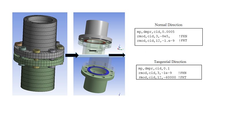
In the Mechanical Application, you can define this type of interface damping by associating command objects with the two contact regions. In the above figure, example command objects used to define the interface damping are shown on the right. See Command Object in the Mechanical User's Guide for more information.
The following topics related to thickness effects are available:
You can account for the thickness of shells (2D and 3D) and beams using KEYOPT(11). (This does not apply to 3D beam-to-beam contact.) For rigid-to-flexible contact, the program automatically shifts the contact surface to the bottom or top of the shell/beam surface. For flexible-to-flexible contact, the program automatically shifts both the contact and target surfaces which are attached to shell/beam elements. By default, the program does not account for the element thickness, and beams and shells are discretized at their mid-surface in which penetration distance is calculated from the mid-surface.
When you set KEYOPT(11) = 1 to account for beam or shell thickness, the contact distance is calculated from either the top or the bottom surface as specified previously in Steps in a Contact Analysis.
Note: Only use KEYOPT(11) = 1 to account for thickness when you have shell or beam elements with nodes located at the middle surface.
When building your model geometry, if you are going to account for thickness, remember the offsets which may come from either the contact surface or target surface or from both. When you specify a contact offset (CNOF) along with setting KEYOPT(11) = 1, it is defined from the top or bottom of the shell/beam, not the mid-surface. When used with SHELL181, SHELL208, SHELL209, SHELL281, or ELBOW290, changes in thickness during deformation are also taken into account.
For line-to-surface contact modeled with CONTA177, KEYOPT(11) is used to account for thickness of beam elements on the contact side and shell elements on the target side. See Accounting for Thickness Effect (KEYOPT(11)) for more information.
When using KEYOPT(11) for shell and beam contact, the penetration and gap distances are always measured from the midsurface of the shell or beam element. Any defined offset of the shell or beam element is ignored by the contact elements.
The following topics concerning time step control and impact constraints are available:
Time step control is an automatic time stepping feature that predicts when the status of a contact element will change and cuts the current time step back.
Impact constraints are used in a transient dynamic analysis to satisfy the momentum and energy balance at the contact and target interface. See Dynamic Contact and Impact Modeling for more information.
Use KEYOPT(7) = 0, 1, 2, or 3 to control time stepping, where KEYOPT(7) = 0 provides no control (the default), and KEYOPT(7) = 3 provides the most control.
KEYOPT(7) = 0: No control. The time step size is unaffected by the prediction. This setting is appropriate for most analyses when automatic time stepping is activated and a small time step size is allowed.
KEYOPT(7) = 1: Time step size is bisected in these circumstances:
If too much penetration occurs during an iteration.
If too much sliding distance occurs when the adaptive small-sliding option is activated (KEYOPT(18) = 2).
If the contact status changes dramatically.
KEYOPT(7) = 2: Predict a reasonable increment for the next substep.
KEYOPT(7) = 3: Predict a minimal time increment for the next substep.
Use KEYOPT(7) = 4 to activate impact constraints.
KEYOPT(7) = 4: Use impact constraints for standard or rough contact (KEYOPT(12) = 0 or 1) in a transient dynamic analysis with automatic adjustment of the time increment.
The surface-to-surface contact and target elements allow birth and death. The elements can be removed for part of an analysis and then reactivated for a later stage. This feature is useful for modeling complex metal forming processes where multiple rigid target surfaces need to interact with the contact surface at different stages of the analysis. For example, springback modeling often requires removing the rigid tools at the end of the forming processes.
Keep the following points in mind when using element birth and death with contact:
Use caution when deactivating target elements (EKILL command) in the beginning of an analysis. In this situation the program no longer traces the initial contact conditions, so the effects of initial penetration or gap (KEYOPT(9) > 0 on the contact element) are not considered even if the target elements are reactivated (EALIVE command) in a later load step.
For the nodal detection methods (KEYOPT(4) > 0), the contact constraint condition can vary from node to node within a killed contact element. Whether the contact constraint on a specific node is active or inactive is highly dependent on the contact element numbering and the birth/death status of adjacent elements.
When using the small-sliding option (KEYOPT(18) = 1 on the contact element), if the contact elements are deactivated (EKILL) in the beginning of the analysis, you must set KEYOPT(9) > 0 in order for contact to be considered once the elements are reactivated (EALIVE). For contact pairs that use projection-based contact (KEYOPT(4) = 3, 4, or 5) in conjunction with the small-sliding option (KEYOPT(18) = 1), you should apply the birth and death options only to the contact elements (not the target elements).
For surface-based constraints, apply the birth and death option only to the pilot node element (target element), not the contact elements.
The birth and death capability requires Newton-Raphson iterations to obtain solution accuracy due to sudden changes in contact conditions. For linear contact models (bonded contact pairs with small deflection) that utilize birth and death, the NROPT,FULL command (full Newton-Raphson procedure) must be specified before the first SOLVE command.