


CONTA172
2D 3-Node
Surface-to-Surface Contact
CONTA172 Element Description
CONTA172 is used to represent contact and sliding between 2D target surfaces (TARGE169) and a deformable surface, defined by this element. The element is applicable to 2D structural and coupled-field contact analyses. It can be used for both pair-based contact and general contact.
In the case of pair-based contact, the target surface is defined by the 2D target element type, TARGE169. In the case of general contact, the target surface can be defined by CONTA172 elements (for deformable surfaces) or TARGE169 elements (for rigid bodies only).
This element is located on the surfaces of 2D solid or shell elements with or without midside nodes (for example, PLANE182, PLANE183, INTER193, SHELL208, SHELL209, PLANE223, CPT213, MATRIX50).
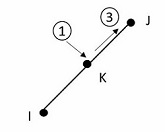
The element has the same geometric characteristics as the solid element face with which it is connected (see Figure 172.1: CONTA172 Geometry). Contact occurs when the element surface penetrates an associated target surface.
Coulomb friction, shear stress friction, user-defined friction
with the USERFRIC subroutine, and user-defined
contact interaction with the USERINTER subroutine
are allowed. This element also allows separation of bonded contact
to simulate interface delamination.
See CONTA172 in the Mechanical APDL Theory Reference for more details about this element. A 3D surface-to-surface contact element (CONTA174) is also available.

CONTA172 Input Data
The geometry and node locations are shown in Figure 172.1: CONTA172 Geometry. The element is defined by three nodes if the underlying elements have midside nodes, or two nodes if the underlying elements do not have midside nodes. See Quadratic Elements (Midside Nodes) in the Modeling and Meshing Guide for more information on the use of midside nodes.
The element x-axis is along the I-J line of the element. The correct node ordering of the contact element is critical for proper detection of contact. The nodes must be ordered such that the target lies to the right side of the contact element when moving from the first contact element node to the second contact element node as in Figure 172.1: CONTA172 Geometry.
Pair-Based Contact versus General Contact
There are two methods to define a contact interaction: the pair-based contact definition and the general contact definition. Both contact definitions can exist in the same model. CONTA172 can be used in either type of contact definition.
The pair-based contact definition is usually more efficient and more robust than the general contact definition; it supports more options and specific contact features.
Pair-Based Contact
In a pair-based contact definition, the 2D contact surface elements (CONTA172) are associated with the 2D target segment elements (TARGE169) via a shared real constant set. The program looks for contact only between surfaces with the same real constant set ID (which is greater than zero). The material ID associated with the contact element is used to specify interaction properties (such as friction coefficient) defined by MP or TB commands.
If more than one target surface will make contact with the same boundary of solid elements, you must define several contact elements that share the same geometry but relate to separate targets (targets with different real constant numbers). Alternatively, you can combine several target surfaces into one (that is, multiple targets sharing the same real constant number). See Identifying Contact Pairs in the Contact Technology Guide for more information.
For either rigid-flexible or flexible-flexible contact, one of the deformable surfaces must be represented by a contact surface. See Designating Contact and Target Surfaces in the Contact Technology Guide for more information.
See Generating Contact Elements in the Contact Technology Guide for information on generating elements automatically using the ESURF command.
General Contact
In a general contact definition, the general contact surfaces are generated automatically by the GCGEN command based on physical parts and geometric shapes in the model. The program overlays contact surface elements (CONTA172) on 2D deformable bodies (on both lower- and higher-order elements) and vertex-to-surface elements (CONTA175) on convex corners of 2D solid bodies and/or shell structures. The general contact definition may also contain target elements (TARGE169) overlaid on the surfaces of standalone rigid bodies.
The GCGEN command automatically assigns section IDs and element type IDs for each general contact surface. As a result, each general contact surface consists of contact or target elements that are easily identified by a unique section ID number. The real constant ID and material ID are always set to zero for contact and target elements in the general contact definition.
The program looks for contact interaction among all surfaces and within each surface. You can further control contact interactions between specific surfaces that could potentially be in contact by using the GCDEF command. The material ID and real constant ID input on GCDEF identify interface properties (defined by MP or TB commands) and contact control parameters (defined by the R command) for a specific contact interaction. Unlike a pair-based contact definition, the contact and target elements in the general contact definition are not associated with these material and real constant ID numbers.
If both pair-based contact and general contact are defined in a model, the pair-based contact definitions are preserved, and the general contact definition automatically excludes overlapping interactions wherever pair-based contact exists.
Some element key options are not used or are set automatically for general contact. See the individual KEYOPT descriptions in "CONTA172 Input Summary" for details.
Friction
To model isotropic friction, use the TB,FRIC,,,,ISO command. You can define a coefficient of friction that is dependent on temperature, time, normal pressure, sliding distance, or sliding relative velocity by using the TBFIELD command along with TB,FRIC,,,,ISO. See Contact Friction in the Material Reference for more information.
To implement a user-defined friction model, use the TB,FRIC command with
TBOPT = USER to specify friction properties and write a
USERFRIC subroutine to compute friction forces. See Writing Your Own Friction Law (USERFRIC) in the Contact Technology Guide for
more information on how to use this feature. See also the Guide to User-Programmable Features in the Programmer's Reference for a detailed description
of the USERFRIC subroutine.
Other Input
The contact interaction subroutine USERINTER is available for
user-defined interface interactions, including interactions in the normal and tangential
directions as well as coupled-field interactions. See Defining Your Own Contact Interaction (USERINTER) in the Contact Technology Guide for more information on
how to use this feature. See also the Guide to User-Programmable Features in the Programmer's Reference for a detailed description of the
USERINTER subroutine.
To model the fluid penetration loads shown in Figure 172.2: Fluid Penetration Pressure Directions, use the SFE command to specify the
fluid pressure values in the normal (LKEY = 1) and tangential
directions (LKEY = 3) in the element coordinate system
(ESYS) and the fluid penetration starting points
(LKEY = 2). For more information, see Applying Fluid-Pressure-Penetration Loads in the Contact Technology Guide.
To model proper momentum transfer and energy balance between contact and target surfaces, impact constraints should be used in transient dynamic analysis. See the description of KEYOPT(7) below and the contact element discussion in the Mechanical APDL Theory Reference for details.
To model separation of bonded contact with KEYOPT(12) = 2, 3, 4, 5, or 6, use the TB command with the CZM label. See Debonding in the Contact Technology Guide for more information.
To model wear at the contact surface, use the TB command with the WEAR label. See Contact Surface Wear in the Contact Technology Guide for more information.
This element supports various 2D stress states, including plane stress, plane strain, and axisymmetric states. The stress state is automatically detected according to the stress state of the underlying element. However, if the underlying element is a superelement, you must use KEYOPT(3) to specify the stress state.
Two types of geometry correction are available for this element: surface smoothing and bolt thread modeling. Surface smoothing is a geometry correction technique that eliminates inaccuracies introduced by linear elements on a curved (circular or nearly circular) contact surface. Bolt thread modeling provides a method for simulating contact between a threaded bolt and bolt hole without having to model the detailed thread geometry. Both of these geometry correction techniques are implemented through section definitions (SECTYPE, SECDATA, and SECNUM commands). For more information, see Geometry Correction for Contact and Target Surfaces in the Contact Technology Guide.
A summary of the element input is given in "CONTA172 Input Summary". A general description of element input is given in Element Input.
Using CONTA172 to Define a Result Section
A result section is a user-defined surface comprised of CONTA172 elements that is used to output and monitor section forces, moments, and other output quantities. See Monitoring Result Section Data During Solution in the Structural Analysis Guide for more information. When this element is used to define a result section, KEYOPT(4) = 1 and 2 are the only applicable key option settings, and no real constants are used. For this special case, the CONTA172 element does not represent contact interaction.
CONTA172 Input Summary
- Nodes
I, J, K
- Degrees of Freedom
Set by KEYOPT(1)
- Real Constants
R1, R2, FKN, FTOLN, ICONT, PINB, PZER, CZER, TAUMAX, CNOF, FKOP, FKT, COHE, TCC, FHTG, SBCT, RDVF, FWGT, ECC, FHEG, FACT, DC, SLTO, TNOP, TOLS, , PPCN, FPAT, COR, STRM, FDMN, FDMT, (Blank), (Blank), TBND, WBID PCC, PSEE, ABPP, FPFT, FPWT, DCC, DCON, ABDC, BSRL, KSYM, TFOR, TEND See Table 172.1: CONTA172 Real Constants for descriptions of the real constants. - Material Properties
TB command: See Element Support for Material Models for this element. MP command: MU, EMIS, DMPR, DMPS - Surface Loads
Pressure, Face 1 (I-J) (opposite to contact normal direction); used for fluid pressure penetration loading. On the SFE command use LKEY= 1 to specify the normal pressure values, and useLKEY= 2 to specify starting and penetrating points. UseLKEY= 3 to specify the tangential pressure values.Convection, Face 1 (I-J-K) Heat Flux, Face 1 (I-J-K) - Special Features
- KEYOPTs
Presented below is a list of KEYOPTS available for this element. Included are links to sections in the Contact Technology Guide where more information is available on a particular topic.
- KEYOPT(1)
Selects degrees of freedom:
- 0 --
UX, UY
- 1 --
UX, UY, TEMP
- 2 --
TEMP
- 3 --
UX, UY, TEMP, VOLT
- 4 --
TEMP, VOLT
- 5 --
UX, UY, VOLT
- 6 --
VOLT
- 7 --
AZ
- 8 --
UX, UY, PRES
- 9 --
UX, UY, PRES, TEMP
- 10 --
PRES
- 11 --
UX, UY, CONC, TEMP
- 12 --
UX, UY, CONC, TEMP, VOLT
- 13 --
UX, UY, CONC
- 14 --
CONC
Note: When the underlying elements are 2D axisymmetric elements with torsion, ROTY (torsion DOF) is automatically added to the existing UX, UY degree of freedom set. ROTY is also added when KEYOPT(3) = 4 and the underlying elements are superelements.
Note: For KEYOPT(1) = 8, 9, and 10, the pore pressure (PRES) degree of freedom is ignored at midside nodes if the underlying element is the higher-order 2D coupled pore-pressure mechanical solid (CPT213).
Note: For general contact, the GCGEN command automatically sets KEYOPT(1) based on the degrees of freedom of the underlying solid or shell elements.
- KEYOPT(2)
Contact algorithm:
- 0 --
Augmented Lagrangian (default)
- 1 --
Penalty function
- 2 --
Multipoint constraint (MPC); see Multipoint Constraints and Assemblies in the Contact Technology Guide for more information
- 3 --
Lagrange multiplier on contact normal and penalty on tangent
- 4 --
Pure Lagrange multiplier on contact normal and tangent
- KEYOPT(3)
Standard KEYOPT(3) Usage
Element stress state. The stress state is detected automatically except when the underlying elements are superelements.
- 0 --
Automatic detection based on underlying element (valid when the underlying elements are not superelements)
- 1 --
Axisymmetric (Use this option only when underlying elements are superelements.)
- 2 --
Plane stress/plane strain with unit thickness (Use this option only when underlying elements are superelements.)
- 3 --
Plane stress with thickness input (Use this option only when underlying elements are superelements.)
- 4 --
Axisymmetric with torsion. ROTY is added to the UX, UY degree of freedom set specified by KEYOPT(1). (Use this option only when underlying elements are superelements.)
Alternate KEYOPT(3) Usage to Control Units of Normal Contact Stiffness
Units of normal contact stiffness:
- 0 --
FORCE/LENGTH3 (default).
- 1 --
FORCE/LENGTH. This option is valid only when a penalty-based algorithm is used (KEYOPT(2) = 0 or 1) and the absolute normal contact stiffness value is explicitly specified (that is, a negative value input for real constant FKN).
Note: KEYOPT(3) is not supported for contact elements used in a general contact definition.
- KEYOPT(4)
Standard KEYOPT(4) Usage
Location of contact detection point:
- 0 --
On Gauss point (for general cases)
- 1 --
On nodal point - normal from contact surface
- 2 --
On nodal point - normal to target surface
- 3 --
On nodal point - normal from contact surface (standard projection-based method)
- 4 --
On nodal point - normal from contact surface (dual shape function projection-based method)
- 5 --
Unified approach that combines Gauss point, normal to target surface, and standard projection methods
Note: Certain restrictions apply when the surface projection-based method (KEYOPT(4) = 3, 4, or 5) is defined. For more information, see Using the Surface Projection-Based Contact Method in the Contact Technology Guide.
Alternate KEYOPT(4) Usage with Surface-Based Constraints
To define a surface-based constraint, set KEYOPT(4) as follows:
- 1 --
Defines a force-distributed constraint. The force-distributed constraint can be based on either the MPC approach (KEYOPT(2) = 2) or the Lagrange multiplier method (KEYOPT(2) = 3).
- 2 --
Defines a rigid surface constraint. The rigid surface constraint can be based on either the MPC approach (KEYOPT(2) = 2) or the Lagrange multiplier method (KEYOPT(2) = 3).
- 3 --
Defines a coupling constraint. The MPC approach (KEYOPT(2) = 2) must be used.
For more information, see Surface-Based Constraints in the Contact Technology Guide.
Alternate KEYOPT(4) Usage with Result Sections
When CONTA172 is used to define a result section, KEYOPT(4) determines how motion of the result section is accounted for in a large deflection analysis:
- 1 --
The anchor point moves and the local coordinate system rotates with the average rigid body motion of the contact elements used to define the result section.
- 2 --
The anchor point moves and the local coordinate system rotates with the average rigid body motion of the underlying elements.
For more information, see Monitoring Result Section Data During Solution in the Structural Analysis Guide.
- KEYOPT(5)
CNOF/ICONT Automated adjustment:
- 0 --
No automated adjustment
- 1 --
Close gap with auto CNOF
- 2 --
Reduce penetration with auto CNOF
- 3 --
Close gap/reduce penetration with auto CNOF
- 4 --
Auto ICONT
- KEYOPT(6)
Normal contact stiffness variation (used to enhance stiffness updating when KEYOPT(10) ≠ 1):
- 0 --
Use default range for stiffness updating
- 1 --
Make a nominal refinement to the allowable stiffness range
- 2 --
Make an aggressive refinement to the allowable stiffness range
- 3 --
Use an exponential pressure-penetration relationship
- KEYOPT(7)
Element level time incrementation control / impact constraints:
- 0 --
No control
- 1 --
Automatic bisection of increment
- 2 --
Change in contact predictions made to maintain a reasonable time/load increment
- 3 --
Change in contact predictions made to achieve the minimum time/load increment whenever a change in contact status occurs
- 4 --
Use impact constraints for standard or rough contact (KEYOPT(12) = 0 or 1) in a transient dynamic analysis with automatic adjustment of time increment
Note: KEYOPT(7) = 4 is not supported for contact elements used in a general contact definition.
- KEYOPT(8)
Symmetric contact behavior:
- 0 --
Both symmetric pairs are active. However, each pair has its own contact characteristics.
- 1 --
Both symmetric pairs are active and have the same contact characteristics.
- 2 --
The program internally selects which asymmetric contact pair is used at the solution stage (used only when symmetric contact is defined). However, the contact stiffness of the active contact pair is influenced by the underlying element stiffness of the inactive pair.
- 3 --
The program internally selects which asymmetric contact pair is used at the solution stage (used only when symmetric contact is defined). The contact characteristics of the active contact pair are completely independent of the inactive pair.
Note: KEYOPT(8) settings are ignored for asymmetric contact pairs and rigid-to-rigid contact pairs.
Note: KEYOPT(8) is ignored for contact elements used in a general contact definition. Instead, use the command GCDEF,AUTO to enable auto-asymmetric pairing logic.
- KEYOPT(9)
Effect of initial penetration or gap:
- 0 --
Include both initial geometrical penetration or gap and offset - 1 --
Exclude both initial geometrical penetration or gap and offset
- 2 --
Include both initial geometrical penetration or gap and offset, but with ramped effects
- 3 --
Include offset only (exclude initial geometrical penetration or gap)
- 4 --
Include offset only (exclude initial geometrical penetration or gap), but with ramped effects
- 5 --
Include offset only (exclude initial geometrical penetration or gap) regardless of the initial contact status (near-field or closed)
- 6 --
Include offset only (exclude initial geometrical penetration or gap), but with ramped effects regardless of the initial contact status (near-field or closed)
Note: The effects of KEYOPT(9) are dependent on settings for other KEYOPTs. The indicated initial gap effect is considered only if KEYOPT(12) = 4 or 5. See the discussion on using KEYOPT(9) in the Contact Technology Guide for more information.
Note: KEYOPT(9) is not supported for contact elements used in a general contact definition. Instead, use the command TBDATA,,
C1in conjunction with TB,INTER to specify the effect of initial penetration or gap. If TBDATA,,C1is not specified, the default for general contact is to exclude initial penetration/gap and offset. For more information, see Interaction Options for General Contact Definitions in the Material Reference.- KEYOPT(10)
Contact stiffness update:
- 0 --
Each iteration based on the current mean stress of underlying elements. The actual elastic slip never exceeds the maximum allowable limit (SLTO) during the entire solution.
- 1 --
Each load step if FKN is redefined during the load step.
- 2 --
Each iteration based on the current mean stress of underlying elements. The actual elastic slip does not exceed the maximum allowable limit (SLTO) within a substep.
- KEYOPT(11)
Beam/Shell thickness effect:
- 0 --
Exclude
- 1 --
Include
- KEYOPT(12)
Behavior of contact surface:
- 0 --
Standard
- 1 --
Rough
- 2 --
No separation (sliding permitted)
- 3 --
Bonded
- 4 --
No separation (always)
- 5 --
Bonded (always)
- 6 --
Bonded (initial contact)
Note: When KEYOPT(12) = 5 or 6 is used with the MPC algorithm to model surface-based constraints, the KEYOPT(12) setting will have an effect on the local coordinate system of the contact element nodes. See Specifying a Local Coordinate System in the Contact Technology Guide for more information.
Note: KEYOPT(12) is not supported for contact elements used in a general contact definition. Instead, use the command TB,INTER with the appropriate
TBOPTlabel to specify the behavior at the contact surface. For more information, see Interaction Options for General Contact Definitions in the Material Reference.- KEYOPT(13)
Tangential contact stiffness variation only for frictional contact.
- 0 --
Use the default range for stiffness updating.
- 1 --
Make an aggressive refinement to the allowable stiffness range.
- KEYOPT(14)
Behavior of fluid pressure penetration load. KEYOPT(14) is valid only if a fluid pressure penetration load (SFE,,,PRES) is applied to the contact element:
- 0 --
Fluid pressure penetration load is applied based on the contact status of the current iteration. Any contact detection point which was previously exposed to the fluid pressure remains in the condition of “penetrating” (default).
- 1 --
Fluid pressure penetration load is applied based on the contact status of the last converged substep. Any contact detection point which was previously exposed to the fluid pressure remains in the condition of “penetrating”.
- 2 --
Fluid pressure penetration load is applied based on the contact status of the current iteration. At each iteration, the fluid pressure penetration load is newly applied from the initial starting points.
- 3 --
Fluid pressure penetration load is applied based on the contact status of the last converged substep. At each iteration, the fluid pressure penetration load is newly applied from the initial starting points.
Note: KEYOPT(14) is not supported for contact elements used in a general contact definition.
- KEYOPT(15)
Effect of contact stabilization damping:
- 0 --
Damping is activated only in the first load step (default).
- 1 --
Deactivate automatic damping.
- 2 --
Damping is activated for all load steps.
- 3 --
Damping is activated at all times regardless of the contact status of previous substeps.
Note: Normal stabilization damping is only applied to the contact element when the current contact status of the contact detection point is near-field. When KEYOPT(15) = 0, 1, or 2, normal stabilization damping is not applied in the current substep if any contact detection point has a closed status. However, when KEYOPT(15) = 3, normal stabilization damping is always applied as long as the current contact status of the contact detection point is near-field. Tangential stabilization damping is automatically activated when normal damping is activated. Tangential damping can also be applied independent of normal damping for sliding contact. See Applying Contact Stabilization Damping in the Contact Technology Guide for more information.
- KEYOPT(18)
Sliding behavior:
- 0 --
Finite sliding (default). The contacting interface can undergo separation, relative large sliding, and arbitrary rotation.
- 1 --
Small sliding. The contacting interface can undergo only small sliding during the entire solution; arbitrary rotation is permitted.
- 2 --
Adaptive small sliding. The contact interface can undergo either small sliding or finite sliding within each substep based on the contact status at the beginning of the substep. If the contact status is closed, small sliding is used.
Table 172.1: CONTA172 Real Constants
| No. | Name | Description | For more information, see this section in the Contact Technology Guide . . . |
|---|---|---|---|
| 1 | R1 |
Target circle radius | |
| 2 | R2 |
Superelement thickness | |
| 3 | FKN | ||
| 4 | FTOLN |
Penetration tolerance factor [5] | |
| 5 | ICONT |
Initial contact closure | |
| 6 | PINB |
Pinball region | or |
| 7 | PZER | Pressure at zero penetration [1] [2] | Pressure-Penetration Relationship (KEYOPT(6) = 3) |
| 8 | CZER | Initial contact clearance | Pressure-Penetration Relationship (KEYOPT(6) = 3) |
| 9 | TAUMAX | ||
| 10 | CNOF | ||
| 11 | FKOP | ||
| 12 | FKT | ||
| 13 | COHE |
Contact cohesion | |
| 14 | TCC | ||
| 15 | FHTG |
Frictional heating factor | |
| 16 | SBCT |
Stefan-Boltzmann constant | |
| 17 | RDVF | ||
| 18 | FWGT |
Heat distribution weighing factor | Modeling Heat Generation Due to Friction (thermal) orHeat Generation Due to Electric Current (electric) |
| 19 | ECC |
Electric contact conductance or electric contact capacitance [1] [2] [4] | |
| 20 | FHEG |
Joule dissipation weight factor | |
| 21 | FACT |
Static/dynamic ratio | |
| 22 | DC |
Exponential decay coefficient | |
| 23 | SLTO |
Allowable elastic slip | |
| 24 | TNOP |
Maximum allowable tensile contact pressure [5] | |
| 25 | TOLS |
Target edge extension factor | |
| 27 | PPCN | ||
| 28 | FPAT |
Fluid penetration acting time | |
| 29 | COR |
Coefficient of restitution | |
| 30 | STRM |
Load step number for ramping penetration or Starting time for contact stiffness ramping | |
| 31 | FDMN | Normal stabilization damping factor [1] [2] | |
| 32 | FDMT | Tangential stabilization damping factor [1] [2] | |
| 35 | TBND | Critical bonding temperature [1] [2] | |
| 36 | WBID | Internal contact pair ID (used by Ansys Workbench) | |
| 37 | PCC | Pore fluid contact permeability coefficient [1] [2] | |
| 38 | PSEE | Pore fluid seepage coefficient [1] [2] | |
| 39 | ABPP | Ambient pore pressure [1] [2] | |
| 40 | FPFT | Gap pore fluid flow participation factor [1] [2] | |
| 41 | FPWT | Gap pore fluid flow distribution weighting factor | |
| 42 | DCC | Contact diffusivity coefficient [1] [2] | |
| 43 | DCON | Diffusive convection coefficient [1] [2] | |
| 44 | ABDC | Ambient concentration [1] [2] | |
| 45 | BSRL | Original contact pair real constant set ID (after contact splitting) | Real Constant Set IDs for Split Pairs |
| 46 | KSYM | Real constant set ID of the associated companion pair for symmetric contact or self contact (after contact splitting) | Real Constant Set IDs for Split Pairs |
| 47 | TFOR | Pair-based force tolerance | Checking Contact Pair-Based Force Convergence |
| 48 | TEND | Ending time for ramping contact stiffness | Modeling Interference Fit |
This real constant can be defined as a function of certain primary variables.
This real constant can be defined by the user subroutine USERCNPROP.F.
When CONTA172 is used as part of a forced-distributed constraint and KEYOPT(7) = 2 on the TARGE169 element, FKN is used to define weighting factors in tabular format with node number as the primary variable.
ECC is electric contact conductance per unit area in a current-based electric analysis, or electric contact capacitance per unit area in a charge-based electric analysis (see Modeling Surface Interaction).
When the relaxation option is enabled (KEYOPT(11) = 1 on the TARGE169 element), FKN and FKT are translational relaxation coefficient and rotational relaxation coefficient, respectively, and tabular input is not supported. In addition, FTOLN and TNOP are translational tolerance and rotational tolerance, respectively.
CONTA172 Output Data
The solution output associated with the element is in two forms:
Nodal displacements included in the overall nodal solution
Additional element output as shown in Table 172.2: CONTA172 Element Output Definitions
A general description of solution output is given in Solution Output. See the Basic Analysis Guide for ways to view results.
The Element Output Definitions table uses the following notation:
A colon (:) in the Name column indicates that the item can be accessed by the Component Name method (ETABLE, ESOL). The O column indicates the availability of the items in the file jobname.out. The R column indicates the availability of the items in the results file.
In either the O or R columns, “Y” indicates that the item is always available, a letter or number refers to a table footnote that describes when the item is conditionally available, and “-” indicates that the item is not available.
Table 172.2: CONTA172 Element Output Definitions gives element output. In the results file, the nodal results are obtained from its closest integration point.
Table 172.2: CONTA172 Element Output Definitions
| Name | Definition | O | R |
|---|---|---|---|
| EL | Element Number | Y | Y |
| NODES | Nodes I, J | Y | Y |
| XC, YC | Location where results are reported | Y | 5 |
| TEMP | Temperatures T(I), T(J) | Y | Y |
| LENGTH | Element length | Y | - |
| VOLU | AREA | Y | Y |
| NPI | Number of integration points | Y | - |
| ITRGET | Target surface number (assigned by the program) | Y | - |
| ISOLID [14] | Underlying solid, shell, or beam element number | Y | - |
| CONT:STAT | Current contact statuses | 1 | 1 |
| OLDST | Old contact statuses | 1 | 1 |
| NX, NY | Surface normal vector components | Y | - |
| ISEG | Current contacting target element number | Y | Y |
| OLDSEG | Underlying old target number | Y | - |
| CONT:PENE | Current penetration (gap = 0; penetration = positive value) | Y | Y |
| CONT:GAP | Current gap (gap = negative value; penetration = 0) | Y | Y |
| NGAP | New or current gap at current converged substep (gap = negative value; penetration = positive value) | Y | - |
| OGAP | Old gap at previously converged substep (gap = negative value; penetration = positive value) | Y | - |
| IGAP | Initial gap at start of current substep (gap = negative value; penetration = positive value) | Y | Y |
| GGAP | Geometric gap at current converged substep (gap = negative value; penetration = positive value) | - | Y |
| CONT:PRES | Normal contact pressure | Y | Y |
| CONT:SFRIC [13] | Tangential contact stress = SQRT(TAUR**2 + TAUS**2) | Y | Y |
| TAUR, TAUS [13] | Tangential contact stresses in 1st slip (XY plane) and 2nd slip (circumferential) | Y | Y |
| KN | Current normal contact stiffness (Force/Length3) | Y | Y |
| KT | Current tangent contact stiffness (Force/Length3) | Y | Y |
| MU | Friction coefficient | Y | Y |
| CONT:SLIDE | Amplitude of total accumulated sliding = SQRT(TASR**2 + TASS**2) | 3 | 3 |
| TASR, TASS [13] | Total (algebraic sum) sliding in 1st slip (XY plane) and 2nd slip (circumferential) | 3 | 3 |
| AASR, AASS [13] | Total (absolute sum) sliding in 1st slip (XY plane) and 2nd slip (circumferential) | 3 | 3 |
| TOLN | Penetration tolerance | Y | Y |
| CONT:STOTAL | Total stress, SQRT (PRES**2 + TAUR**2 + TAUS**2) | Y | Y |
| FDDIS | Frictional energy dissipation rate | 6 | 6 |
| ELSI | Total elastic slip distance | - | Y |
| PLSI | Total accumulated plastic slip due to frictional sliding | - | Y |
| GSLID | Algebraic sum sliding | - | 7 |
| VREL | Sliding velocity (slip rate) | - | Y |
| DBA | Penetration variation | Y | Y |
| PINB | Pinball Region | - | Y |
| CONT:CNOS | Total number of contact status changes during substep | Y | Y |
| TNOP | Maximum allowable tensile contact pressure | Y | Y |
| SLTO | Allowable elastic slip | Y | Y |
| CAREA | Contacting area | - | Y |
| CONT:FPRS | Actual applied fluid penetration pressure (magnitude of normal and tangential) | - | Y |
| FPRSN | Actual applied fluid penetration normal pressure | - | Y |
| FPTP | Actual applied fluid penetration tangential pressure | - | Y |
| FSTART | Fluid penetration starting time | - | Y |
| DTSTART | Load step time during debonding | Y | Y |
| DPARAM | Debonding parameter | Y | Y |
| DENERI [10] | Energy released due to separation in normal direction - mode I debonding | Y | Y |
| DENERII [10] | Energy released due to separation in tangential direction - mode II debonding | Y | Y |
| DENER [11] | Total energy released due to debonding | Y | Y |
| CNFX [8] | Contact element force - X component | - | 4 |
| CNFY [8] | Contact element force - Y component | - | 4 |
| CNFZ [13] | Contact element moment - Y component | - | 4 |
| CNTX [9] | Contact element force due to tangential stresses - X component | - | 4 |
| CNTY [9] | Contact element force due to tangential stresses - Y component | - | 4 |
| CNTZ [13] | Contact element moment due to tangential stresses - Y component | - | 4 |
| SDAMP | Stabilization damping coefficient | - | Y |
| WEARX, WEARY | Wear correction - X and Y components | - | Y |
| VWEAR [12] | Volume lost due to wear | - | Y |
| CONV | Convection coefficient | Y | Y |
| RAC | Radiation coefficient | Y | Y |
| TCC | Conductance coefficient | Y | Y |
| TEMPS | Temperature at contact point | Y | Y |
| TEMPT | Temperature at target surface | Y | Y |
| FXCV | Heat flux due to convection | Y | Y |
| FXRD | Heat flux due to radiation | Y | Y |
| FXCD | Heat flux due to conductance | Y | Y |
| CONT:FLUX | Total heat flux at contact surface | Y | Y |
| FXNP | Flux input | - | Y |
| CNFH | Contact element heat flow | - | Y |
| JCONT | Contact current density (Current/Unit Area) | Y | Y |
| CCONT | Contact charge density (Charge/Unit Area) | Y | Y |
| HJOU | Contact power/area | Y | Y |
| ECURT | Current per contact element | - | Y |
| ECHAR | Charge per contact element | - | Y |
| ECC | Electric contact conductance (for electric current DOF), or electric contact capacitance per unit area (for piezoelectric or electrostatic DOFs) | Y | Y |
| VOLTS | Voltage on contact nodes | Y | Y |
| VOLTT | Voltage on associated target | Y | Y |
| PCC | Pore fluid contact permeability coefficient | Y | Y |
| PSEE | Pore fluid seepage coefficient | Y | Y |
| PRESS | Pore pressure on contact nodes | Y | Y |
| PREST | Pore pressure on associated target | Y | Y |
| PFLUX | Pore volume flux density per unit area flow into contact surface | Y | Y |
| EPELX | Pore volume flux per contact element | - | Y |
| DCC | Contact diffusivity coefficient | Y | Y |
| DCON | Diffusive convection coefficient | Y | Y |
| CONCS | Concentration on contact nodes | Y | Y |
| CONCT | Concentration on associated target | Y | Y |
| DFLUX | Diffusion flux density per unit area flow into contact surface | Y | Y |
| EDELX | Diffusion flux per contact element | - | Y |
The possible values of STAT and OLDST are:
-3 = Closed and sticking (MPC bonded) but overconstrained -2 = Closed and sliding (MPC no separation) but overconstrained 0 = Open and not near contact 1 = Open but near contact 2 = Closed and sliding 3 = Closed and sticking The program will evaluate model to detect initial conditions.
Only accumulates the sliding for sliding and closed contact (STAT = 2,3).
Contact element forces are defined in the global Cartesian system.
Available only at centroid as a *GET item.
FDDIS = (contact friction stress)*(sliding distance of substep)/(time increment of substep)
Accumulated sliding distance for near-field, sliding, and closed contact (STAT = 1,2,3).
The contact element force values (CNFX, CNFY) are calculated based on the individual contact element plus the surrounding contact elements. Therefore, the contact force values may not equal the contact element area times the contact pressure (CAREA * PRES).
CNTX and CNTY report the total contact element forces due to tangential stresses. Since CNFX and CNFY report the total contact element forces, the contact element forces due to normal pressure are (CNFX - CNTX) and (CNFY - CNTY).
DENERI and DENERII are available only when one of the following material models is used: TB,CZM,,,,CBDD or TB,CZM,,,,CBDE.
DENER is available only when one of the following material models is used: TB,CZM,,,,BILI or TB,CZM,,,,EXPO.
The wear volume lost (VWEAR) is calculated based on the individual contact element plus the surrounding contact elements. Therefore, the wear volume may not equal the contact element area times the wear amount in the contact normal direction (CAREA * Wear).
Circumferential components (TAUS, TASR, AASR, CNFZ, CNTZ) are only available when the stress state is axisymmetric with torsion.
The underlying element (ISOLID) can be obtained by a *GET command following a CNCHECK command. See Designating Contact and Target Surfaces for detail.
Note: Contact results (including all element results) are generally not reported for elements that have a status of "open and not near contact" (far-field).
Table 172.3: CONTA172 Item and Sequence Numbers lists output available through the ETABLE command using the Sequence Number method. See Creating an Element Table in the Basic Analysis Guide and The Item and Sequence Number Table in this reference for more information. The following notation is used:
- Name
output quantity as defined in the Table 172.2: CONTA172 Element Output Definitions
- Item
predetermined Item label for ETABLE command
- E
sequence number for single-valued or constant element data
- I, J
sequence number for data at nodes I, J
Table 172.3: CONTA172 Item and Sequence Numbers
| Output Quantity Name | ETABLE and ESOL Command Input | |||
|---|---|---|---|---|
| Item | E | I | J | |
| PRES | SMISC | 5 | 1 | 2 |
| TAUR | SMISC | - | 3 | 4 |
| TAUS | SMISC | - | 24 | 25 |
| FLUX [3] | SMISC | - | 6 | 7 |
| FDDIS [3] | SMISC | - | 8 | 9 |
| FXCV [3] | SMISC | - | 10 | 11 |
| FXRD [3] | SMISC | - | 12 | 13 |
| FXCD [3] | SMISC | - | 14 | 15 |
| FXNP | SMISC | - | 16 | 17 |
| JCONT/CCONT/PFLUX [3] | SMISC | - | 18 | 19 |
| HJOU | SMISC | - | 20 | 21 |
| DFLUX [3] | SMISC | - | 22 | 23 |
| STAT [1] | NMISC | 19 | 1 | 2 |
| OLDST | NMISC | - | 3 | 4 |
| PENE [2] | NMISC | - | 5 | 6 |
| DBA | NMISC | - | 7 | 8 |
| TASR | NMISC | - | 9 | 10 |
| TASS | NMISC | - | 98 | 99 |
| KN | NMISC | - | 11 | 12 |
| KT | NMISC | - | 13 | 14 |
| TOLN | NMISC | - | 15 | 16 |
| IGAP | NMISC | - | 17 | 18 |
| PINB | NMISC | 20 | - | - |
| CNFX | NMISC | 21 | - | - |
| CNFY | NMISC | 22 | - | - |
| CNFZ | NMISC | 96 | - | - |
| CNTX | NMISC | 91 | - | - |
| CNTY | NMISC | 92 | - | - |
| CNTZ | NMISC | 97 | - | - |
| ISEG [4] | NMISC | - | 23 | 24 |
| AASR | NMISC | - | 25 | 26 |
| AASS | NMISC | - | 100 | 101 |
| CAREA | NMISC | 27 | 28 | 89 |
| MU | NMISC | - | 29 | 30 |
| DTSTART | NMISC | - | 31 | 32 |
| DPARAM | NMISC | - | 33 | 34 |
| FPRSN | NMISC | - | 35 | 36 |
| TEMPS | NMISC | - | 37 | 38 |
| TEMPT | NMISC | - | 39 | 40 |
| CONV | NMISC | - | 41 | 42 |
| RAC | NMISC | - | 43 | 44 |
| TCC | NMISC | - | 45 | 46 |
| CNFH | NMISC | 47 | - | - |
| ECURT/ECHAR/EPELX | NMISC | 48 | - | - |
| ECC/PCC/PSEE | NMISC | - | 49 | 50 |
| VOLTS/PRESS | NMISC | - | 51 | 52 |
| VOLTT/PREST | NMISC | - | 53 | 54 |
| CNOS | NMISC | - | 55 | 56 |
| TNOP | NMISC | - | 57 | 58 |
| SLTO | NMISC | - | 59 | 60 |
| DCC | NMISC | - | 61 | 62 |
| CONCS | NMISC | - | 63 | 64 |
| CONCT | NMISC | - | 65 | 66 |
| ELSI | NMISC | - | 67 | 68 |
| DENERI or DENER | NMISC | - | 69 | 70 |
| DENERII | NMISC | - | 71 | 72 |
| FSTART | NMISC | - | 73 | 74 |
| GGAP | NMISC | - | 75 | 76 |
| VREL | NMISC | - | 77 | 78 |
| SDAMP | NMISC | - | 79 | 80 |
| PLSI | NMISC | - | 81 | 82 |
| GSLID | NMISC | - | 83 | 84 |
| WEARX | NMISC | - | 85 | 86 |
| WEARY | NMISC | - | 87 | 88 |
| VWEAR | NMISC | 93 | - | - |
| EDELX | NMISC | 90 | - | - |
| FPTP | NMISC | - | 94 | 95 |
Element Status = highest value of status of integration points within the element
A positive value of flux corresponds to flow into the contact surface.
The floating point output format for large integers may lead to incorrect ISEG values. You should verify the NMISC values via the *GET command. For example, *GET,
Par,ELEM,N,NMISC,23 returns the ISEG value for node I of elementN.
You can display or list contact results through several POST1 postprocessor commands. The contact specific items for the PLNSOL, PLESOL, PRNSOL, and PRESOL commands are listed below:
| STAT | Contact status |
| PENE | Contact penetration |
| PRES | Contact pressure |
| SFRIC | Contact friction stress |
| STOT | Contact total stress (pressure plus friction) |
| SLIDE | Contact sliding distance |
| GAP | Contact gap distance |
| FLUX | Total heat flux at contact surface |
| CNOS | Total number of contact status changes during substep |
| FPRS | Actual applied fluid penetration pressure |
CONTA172 Assumptions and Restrictions
The 2D contact element must be defined in the global X-Y plane as shown in Figure 172.1: CONTA172 Geometry, and the Y-axis must be the axis of symmetry for axisymmetric analyses.
An axisymmetric structure should be modeled in the +X quadrants.
This 2D contact element works with any 3D elements in your model.
Do not use this element in any model that contains axisymmetric harmonic elements.
Node numbering must coincide with the external surface of the underlying solid element or with the original elements comprising the superelement.
This element is nonlinear and requires a full Newton iterative solution, regardless of whether large or small deflections are specified. An exception to this is when MPC bonded contact is specified (KEYOPT(2) = 2 and KEYOPT(12) = 5 or 6).
The normal contact stiffness factor (FKN) must not be so large as to cause numerical instability.
FTOLN, PINB, and FKOP can be changed between load steps or during restart stages.
You can use this element in nonlinear static or nonlinear full transient analyses. In addition, you can use it in modal analyses, eigenvalue buckling analyses, and harmonic analyses. For these analysis types, the program assumes that the initial status of the element (that is, the status at the completion of the static prestress analysis, if any) does not change.
When nodal detection is used and the contact node is on the axis of symmetry in an axisymmetric analysis, the contact pressure on that node is not accurate since the area of the node is zero. The contact force is accurate in this situation.
It is possible for the midside node of the contact element to be in contact while the end nodes (I and J) are not in contact. Because the program reports contact results only for the end nodes, the element may have a closed contact status even though the reported contact pressure is zero. To verify the contact status for contact elements in this situation, list the following ETABLE quantities: SMISC,5 (PRES); NMISC,19 (STAT); NMISC,21 (CNFX); and NMISC,22 (CNFY).
Only damping defined via KEYOPT(15) is supported. All other damping specifications (Rayleigh damping, DMPSTR, and so on) are not supported.
Certain contact features are not supported when this element is used in a general contact definition. For details, see General Contact in the Contact Technology Guide.
CONTA172 Product Restrictions
When used in the product(s) listed below, the stated product-specific restrictions apply to this element in addition to the general assumptions and restrictions given in the previous section.
Ansys Mechanical Pro —
The AZ DOF (KEYOPT(1) = 7) is not available.
Birth and death is not available.
Debonding is not available.
User-defined contact is not available.
User-defined friction is not available.
Ansys Mechanical Premium —
The AZ DOF (KEYOPT(1) = 7) is not available.
Debonding is not available.
User-defined contact is not available.
User-defined friction is not available.