


Pressure-penetration loads can simulate surrounding fluid or air penetrating into the contact interface, based on the contact status. You can apply pressure-penetration loads to flexible-to-flexible or rigid-to-flexible contact pairs. 2D and 3D surface-to-surface contact elements (CONTA172, CONTA174) support pressure-penetration loading.
Fluid pressure along normal and tangential directions can penetrate into the contact interface from one or multiple locations. The fluid-pressure-penetration load has a path-dependent nature. The penetrating path can propagate and vary, and it is determined iteratively. At the beginning of each iteration, the program first detects starting points which are exposed to the fluid pressure. Among the starting points, the program then finds fluid penetrating points where the contact status is open or lost, or where the contact pressure is smaller than the user-defined pressure-penetration criterion. When a contact detection point has a contact condition of "penetrating," it is subjected to the fluid pressure, and its nearest neighboring nodes are considered to be the starting points which are exposed to the fluid pressure as well.
The fluid pressure is not applied to an area having a contact status of open unless the edges/ends of the area belong to the starting points.

The fluid pressure starts to penetrate into the interface between contact and target surfaces from the penetrating points. The fluid penetration can be cut off when contact between the surfaces is reestablished or when contact pressure (normal only) is larger than the fluid penetration criterion.
To model fluid penetration loads, you need to specify the following quantities:
An example analysis showing how to apply fluid penetrating loading is presented in Appendix A: Example 2D Contact Analysis with Fluid Pressure-Penetration Loading.
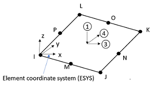
The fluid pressure must be applied to contact and target elements using the SFE command. See Figure 3.41: Fluid Penetration Pressure Directions on CONTA174 and TARGE170 and Figure 3.42: Fluid Penetration Pressure Directions on CONTA172 and TARGE169 for possible fluid penetration pressure directions.
When fluid pressure is applied to the target elements, you must also set KEYOPT(10) = 1 for the target element type.
For 3D contact (contact element CONTA174 and target element TARGE170) use the SFE command as follows:
Set LKEY = 1 to specify the normal
pressure values:
SFE,ELEM,1,PRES,,VAL1,VAL2,VAL3,VAL4
Set LKEY = 3 to specify the
tangential pressure values along x direction of ESYS:
SFE,ELEM,3,PRES,,VAL1,VAL2,VAL3,VAL4
Set LKEY = 4 to specify the
tangential pressure values along y direction of ESYS:
SFE,ELEM,4,PRES,,VAL1,VAL2,VAL3,VAL4
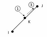
For 2D contact (contact element CONTA172 and target element TARGE169) use the SFE command as follows:
Set LKEY = 1 to specify the normal
pressure values:
SFE,ELEM,1,PRES,,VAL1,VAL2
Set
LKEY = 3 to specify the tangential pressure
values:
SFE,ELEM,3,PRES,,VAL1,VAL2
The pressure is applied only on the corner nodes of the contact and target
elements. The pressure on the midside nodes of CONTA172,
CONTA174, TARGE169, and
TARGE170 is averaged using the pressures of two
adjacent corner nodes. VAL3 and
VAL4 are not used for 2D contact and target
elements.
Pressure value VALi, which is applied to the ith node (where i = 1, 2, 3, 4
indicates node I, J, K, L, respectively) of the contact or target element, can be a constant
numerical value or a table name. If it is constant, the magnitude of pressure is
step-applied or ramped based on the KBC command setting. To specify a
table, enclose the table name in percent signs (%tabname%). Use
the *DIM command to define the table. Only one table can be specified,
and it must be specified in the VAL1 position. Tables specified
in the VAL2, VAL3, and
VAL4 positions are ignored.
The fluid-pressure-penetration load is automatically applied to the penetrating points on contact and target surfaces based on the contact status and the value of KEYOPT(14) of the contact elements.
When KEYOPT(14) = 0 (default) or 2, the fluid-pressure-penetration load varies during iterations based on the current contact status. In certain cases, this can cause an unstable convergence pattern since the contact status and the resulting applied fluid penetration load keep changing during iterations.
When KEYOPT(14) = 1 or 3, the fluid-pressure-penetration load is applied to the contact and target elements based on the contact status at the beginning of each substep and remains constant over that substep even if the contact status keeps changing during iterations. Small increments are often needed to obtain accurate results.
When KEYOPT(14) = 0 or 1, any contact detection point which was previously exposed to the fluid pressure remains in the condition of “penetrating” unless the closed contact condition is reestablished. This is a type of history-dependent loading. The penetrating load may be cut off in the middle of the path.
When KEYOPT(14) = 2 or 3, the fluid-pressure-penetration load is always newly applied from the initial starting points regardless of the history of “penetrating” conditions. Therefore, the penetrating path must be continuous following any starting point.
Keep the following points in mind when defining fluid penetration loads:
For flexible-to-flexible contact with a symmetric contact pair definition (including a self-contact pair), apply the fluid pressure only to the contact elements. You should also set contact element KEYOPT(8) = 1, particularly when fluid-pressure penetration is based on a user-defined pressure-penetration criterion. Setting KEYOPT(8) = 1 for the symmetric pair definition ensures both contact pairs use the same contact characteristics and results in a more accurate contact pressure distribution.
For flexible-to-flexible contact with an asymmetric contact pair definition, you should generally apply fluid pressure on both contact and target elements which are currently or will potentially be exposed to the surrounding fluid. The program ignores fluid penetration loads applied to a target surface if there are no fluid penetration loads applied to the associated contact surface within the contact pair. When the fluid pressures are applied to both contact and target elements, the program has to identify the penetration paths for both the contact surface and the target surface. The iterative process of determining the penetration path on the target surface is very time-consuming, particularly for 3D contact models. Therefore, a symmetric contact pair definition (along with KEYOPT(8) = 1) is recommended as it does not require the specification of fluid penetration pressure on the target surface.
For rigid-to-flexible contact, you should apply the fluid pressure only to the contact elements. The program automatically applies equivalent forces to the rigid target surface to balance out the applied pressure on the contact surface. Fluid pressure applied to the rigid target surface is ignored.
For situations in which multiple contact pairs are defined on the same surface, contact elements may overlap each other. In this case, be careful to apply the fluid penetration pressure only once in areas where contact elements overlap.
The fluid penetration pressure can only be applied to the contact and target elements using the SFE command. Other pressure load commands (SF, SFL, SFA) cannot be used. In addition, you should not apply the pressure on the underlying elements.
The program ignores any fluid penetration pressures applied to MPC based contact pairs.
The effects of pressure load stiffness are automatically included. If an unsymmetric matrix is needed to achieve convergence for pressure load stiffness effects, issue the NROPT,UNSYM command.
When a fluid-pressure-penetration load is applied, the fluid pressure penetrates to the surface from defined starting points. There can be one or multiple starting points. The program automatically finds the default starting points by selecting free end points of 2D contact/target surfaces or nodes of free open edges on 3D contact/target surfaces ("free" meaning that the element is not fully surrounded by adjacent elements, as shown in the figure below).
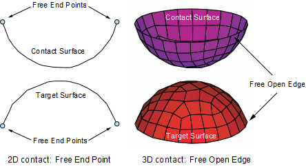
The starting points are initially exposed to the fluid and are potentially
subjected to the penetration pressure. There are no default starting points if the
contact or target surface is continuous with a closed loop. The default starting
points can be overwritten using the SFE command. You can specify
starting points, specify penetrating points, and remove the default starting points
with the SFE command and STAi values,
as described below. Be sure to set LKEY = 2 on the
SFE command in order to specify the
STAi settings. The command format is:
SFE,ELEM,2,PRES,,STA1,STA2,STA3,STA4
STAi = 0 (default) | The program determines whether the ith node is a starting point based on the contact status. The ith node can be a default starting point if the node is a 2D free point or is on a 3D free edge. |
STAi = 1 | The ith node is the starting point which is initially exposed to the fluid. It can be a penetrating point if the initial contact status is "open." The node may no-longer be the starting point when the contact status changes during the deformation process. |
STAi = 2 | The ith node is a penetrating point. The node is always subjected to the fluid pressure in spite of any contact status change. |
STAi = -1 | The ith node is not a default starting point even though it belongs to a 2D free point or a 3D free edge node. |
STAi = -2 | The ith node is a non-penetrating point. The node is never subjected to the fluid pressure in spite of any contact status. |
Note: If only STA1 is specified and the other
STAi values are blank,
STA2, STA3, and
STA4 default to
STA1.
If you intend to define your own starting points, be sure to first suppress all default starting points for all contact and target elements by issuing the following command:
SFE,ALL,2,PRES,,-1
You can specify a pressure-penetration criterion using the contact element real constant PPCN. When the contact pressure is less than the criterion, the starting point turns into the penetrating point. That is, fluid pressure starts to penetrate. Thus, a higher criterion value allows the fluid to penetrate more easily. When the contact pressure is greater than the criterion, the penetrating point returns back to the starting point. That is, fluid penetration is cut off. By default, the penetration criterion (PPCN) is zero. In this case the fluid penetration occurs only when the contact is open, and the cutoff of fluid penetration occurs only when the contact is reestablished.
You can input PPCN as a constant value or as a table of values. The tabular input
can be a function of initial contact detection point location (at the beginning of
solution), contact pressure (positive index values for PRESSURE), geometric
penetration (positive index values for GAP), time, or temperature. To input a table
name, you must enclose the name in % symbols (%tabname%).
Use the *DIM command to define the table. For more information,
see Defining Real Constants in Tabular Format.
The user subroutine USERCNPROP.F is also available for
defining PPCN. To use this subroutine, you must specify the table name %_CNPROP% as
the real constant value. For more information, see Defining Real Constants via a User Subroutine.
When the fluid-pressure penetration occurs, the fluid pressure is applied normal and/or tangential to the contact/target surfaces. As with conventional pressure loading, the current amount of fluid pressure at a given substep depends on whether the pressure is input as a constant value or a table of values, and whether the fluid pressure is ramp- or step-applied (KBC command). If the total amount of fluid pressure is applied instantaneously, convergence difficulties may arise due to large changes in stresses near the contact interface. This is also true when the fluid penetration pressure is removed instantaneously, as when the fluid penetration is cut off. To help stabilize the solution, the program offers an option to ramp the fluid pressure linearly over a time period, during one or several substeps.
To implement this ramping option, specify the fluid penetration acting time using the contact element real constant FPAT. Input a positive number to define the fraction of the time increment of the load step. Input a negative number to define the absolute acting time. The default penetration acting time is 0.01 times the time increment of the current load step.
At each penetrating point, if the time increment of the current substep is less than the fluid penetration acting time (FPAT > (tn - tn-1)), the fluid pressure is ramped up linearly from the actual applied pressure of the previous substep to the full current amount of the fluid pressure over the penetration acting time period. Otherwise (FPAT ≤ (tn - tn-1)), the full amount of current fluid pressure is applied. (See figures below.) At the pressure-penetration cutoff points, if the time increment of the current substep is less than the fluid penetration acting time, the fluid pressure is ramped down linearly from the applied pressure of the previous substep to a zero magnitude over the penetration acting time period. Otherwise, the fluid pressure is immediately removed.


You can redefine or modify fluid-pressure-penetration loads and fluid penetration starting points between load steps using the SFE command.
You can also modify the pressure-penetration criterion (real constant PPCN) and acting time (real constant FPAT) using the RMODIF command.
To remove a fluid-pressure-penetration load, use one of the following methods:
Because these methods remove the fluid penetration pressure immediately,
convergence difficulties may occur. To avoid this problem you can add an extra load
step which applies a small fluid pressure (for example,
VALi = 1e-8) via the SFE command
instead of removing the pressure.
You can list and display the actual fluid penetration pressure applied on contact and target elements using FPRS as a contact result item on the PLNSOL, PLESOL, PRNSOL, and PRESOL commands. For example:
PLESOL,CONT,FPRS
PLNSOL,CONT,FPRS
Using these commands, the reported fluid penetration pressure FPRS is the magnitude of the normal and tangential pressure.
You can use the ETABLE command to access the following fluid penetration pressure quantities applied on contact and target elements: