


A surface-based constraint can be used to couple the motion of nodes on the contact surface to a single pilot node on the target surface. The multipoint constraint (MPC) capability of the contact elements (KEYOPT(2) = 2) allows you to define three types of surface-based constraints:
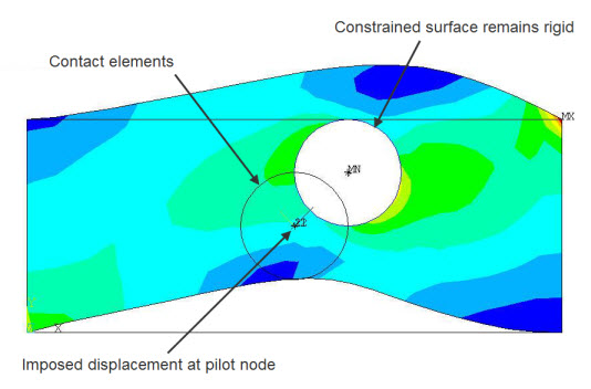
Rigid surface constraint - In this type of constraint, the contact nodes are constrained to the rigid-body motion defined by the pilot node (see Figure 10.7: Rigid Surface Constraint), similar to a constraint defined via CERIG.
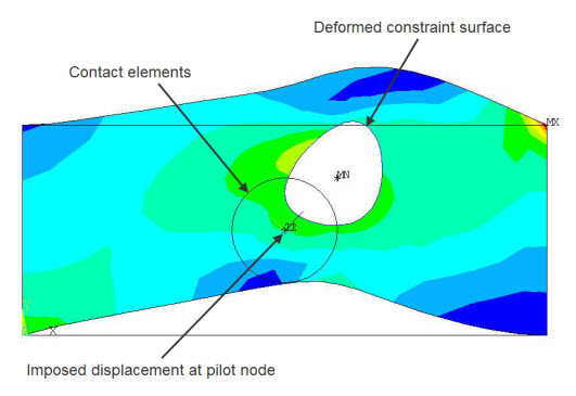
Force-distributed constraint - In this type of constraint, forces or displacements applied on the pilot node are distributed to contact nodes (in an average sense) through shape functions (see Figure 10.8: Force-Distributed Constraint), similar to a constraint defined via RBE3, as described in Force-distributed Constraint Theory Background.
Coupling constraint - In this type of constraint, the degrees of freedom of contact nodes are constrained to have the same solution as the degrees of freedom of the pilot node (see Figure 10.9: Coupling Constraint), similar to a constraint defined via CP.
Note: For the rigid surface constraint and the force-distributed constraint, you can use either the MPC approach (KEYOPT(2) = 2) or the Lagrange multiplier formulation (KEYOPT(2) = 3) to define the constraint.
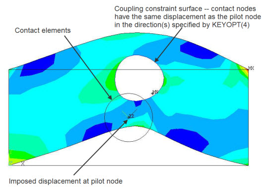
In Figure 10.9: Coupling Constraint, the pilot node's x-direction has been rotated by 45 degrees. Only UX is included in the coupling constraint, so UY on the contact nodes are left free. The resulting deformation shows that UX (rotated 45 degrees from global x) is constant on the contact nodes, but UY is nonuniform.
These surface-based constraints can be used in the following applications:
To apply loads and boundary conditions to the pilot node (such as torque load or drill rotation). Example: a bolt head submitted to a torque force using a force-distributed constraint.
To model rigid bodies. Example: rigid-body definition in multi-body dynamics.
To model rigid end conditions. Example: using a rigid surface constraint to model a rigid end plate or rigid plane section of 3D solid elements.
To model interactions with other joints. Example: two flexible parts linked by a hinge. This can be modeled by two force-distributed constraint definitions whose pilot nodes are connected by a revolute joint element.
To define transitions between solid and structure elements. Example: a beam element connected to a solid element face.
The following surface-based constraint topics are available:
- 10.3.1. Defining Surface-Based Constraints
- 10.3.2. Defining Influence Range (PINB)
- 10.3.3. Degrees of Freedom of Surface-Based Constraints
- 10.3.4. Specifying a Local Coordinate System
- 10.3.5. Additional Guidelines for a Force-Distributed Constraint
- 10.3.6. Additional Guidelines for a Rigid Surface Constraint
- 10.3.7. Additional Guidelines for a Coupling Constraint
- 10.3.8. Modeling a Beam-Solid Assembly
- 10.3.9. Force-distributed Constraint Theory Background
The contact surface can be generated via ESURF. The contact nodes on the contact surface are the dependent nodes of the MPC equations. The pilot node is the only target segment on the target surface side. It is the independent node of the MPC equations. Forces and displacements can be applied on the pilot node and the contact nodes. You can define a follower element (FOLLW201) on the pilot node so that the element-specified external forces and moments on the follower element will follow the motion of the pilot node.
For a force-distributed constraint, use the following contact element key options:
| Force-distributed Constraint KEYOPT Settings (MPC Approach) | |
| KEYOPT(2) = 2 | MPC based approach |
| KEYOPT(12) = 5 or 6 | Bonded always or bonded initial |
| KEYOPT(4) = 1 | Indicates a force-distributed constraint for CONTA172, CONTA174, CONTA175, and CONTA177 |
| Force-distributed Constraint KEYOPT Settings (Lagrange Multiplier Method) | |
| KEYOPT(2) = 3 | Lagrange multiplier method |
| KEYOPT(12) = 5 or 6 | Bonded always or bonded initial |
| KEYOPT(4) = 1 | Indicates a force-distributed constraint for CONTA172, CONTA174, CONTA175, and CONTA177 |
For a rigid surface constraint, use the following contact element key options:
| Rigid Surface Constraint KEYOPT Settings (MPC Approach) | |
| KEYOPT(2) = 2 | MPC based approach |
| KEYOPT(12) = 5 or 6 | Bonded always or bonded initial |
| KEYOPT(4) = 2 | Indicates a rigid surface constraint for CONTA172 and CONTA174 |
| KEYOPT(4) = 0 | Indicates a rigid surface constraint for CONTA175 and CONTA177 |
| Rigid Surface Constraint KEYOPT Settings (Lagrange Multiplier Method) | |
| KEYOPT(2) = 3 | Lagrange multiplier method |
| KEYOPT(12) = 5 or 6 | Bonded always or bonded initial |
| KEYOPT(4) = 2 | Indicates a rigid surface constraint for CONTA172 and CONTA174 |
| KEYOPT(4) = 0 | Indicates a rigid surface constraint for CONTA175 and CONTA177 |
For a coupling constraint, use the following contact element key options:
| Coupling Constraint KEYOPT Settings | |
| KEYOPT(2) = 2 | MPC based approach |
| KEYOPT(12) = 5 or 6 | Bonded always or bonded initial |
| KEYOPT(4) = 3 | Indicates a coupling constraint for CONTA172, CONTA174, CONTA175, and CONTA177 |
The following contact element key options are ignored for surface-based constraints: KEYOPT(8), KEYOPT(5), KEYOPT(7), KEYOPT(10).
In general, PINB is the only contact element real constant used for surface-based constraints. Another exception is the use of real constants FKN, FKT, FTOLN, and TNOP as translational and rotational relaxation coefficients and tolerances when the relaxation method is activated.
The following target element (TARGE169 and TARGE170) key options are applicable to surface-based constraint:
| Target Element KEYOPT Settings | |
| KEYOPT(4) | DOF set to be constrained |
| KEYOPT(6) | Symmetry condition control (used for force-distributed constraints and rigid surface constraints) |
| KEYOPT(7) | Weighting factor control (used only for force-distributed constraints) |
| KEYOPT(10) | Stress-stiffening control for force-distributed constraints and rigid surface constraints defined by the MPC approach. Set KEYOPT(10) = 1 to include stress-stiffening effects. |
Including Stress-Stiffening Effects for Surface-Based Constraints
Stress stiffening effects are automatically included for forced-distributed constraints and rigid surface constraints defined with the Lagrange multiplier method. When these constraint types are defined with the MPC approach, you must set KEYOPT(10) = 1 on the target element to include stress-stiffening effects.
When stress-stiffening effects are included, you can request constraint forces via the NLHIST command.
Including Thermal Expansion Effects for Rigid Surface Constraints
Thermal expansion effects can be included for rigid surface constraints (contact element KEYOPT(4) = 2) defined via CONTA172 or CONTA174 elements. Both the MPC approach and the Lagrange multiplier method are supported. To include thermal expansion effects, you must:
Set KEYOPT(12) = 1 on the target element.
Define the coefficient of thermal expansion using the command MP,ALPX, and assign the material property to the contact and target elements.
Be sure to apply thermal loads on both the pilot node and the contact/target (rigid body) nodes as needed.
By default, all the contact nodes are included in the surface-based constraints. You can select a subset of nodes from these contact nodes by defining a radius of influence range, input as real constant PINB. The nodes that lie within the spherical range (radius = PINB) centered about the pilot node are selected for the definition of the surface-based constraints.
When an influence range is applied to a force-distributed constraint, contact elements within the range are selected first. Then constraints are built between the pilot node and the contact nodes of the selected elements.
This approach is useful when boundary conditions or other constraints (CE/CP) are applied somewhere on the surface involved in the surface-based constraint. By limiting the nodes that are considered to those within the PINB radius, nodes that might be involved in other constraints are excluded and overconstraint is avoided.
Use KEYOPT(1) of the contact elements to specify the degrees of freedom to be used in the constraint set. You may include other field degrees of freedom in addition to the structural DOFs.
The pilot node has both translational and rotational degrees of freedom. The active degrees of freedom at the pilot node depend on the defined type of target elements. Use TARGE169 for 2D surface-based constraints that contain UX, UY, and ROTZ degrees of freedom. Use TARGE170 for 3D surface-based constraints that contain UX, UY, UZ, and ROTX, ROTY, ROTZ degrees of freedom. Generally, you should always set KEYOPT(2) = 1 for the target element to indicate that boundary conditions for rigid target nodes will be user-specified. Otherwise, the program may apply internal constraints on the pilot node.
The degrees of freedom of the surface-based constraints can also be controlled by using KEYOPT(4) of the target element (TARGE169 or TARGE170). For example, for the 3D case (TARGE170), you might specify that only UX, UY, and ROTZ be used in the constraint. You can do this by entering a six digit value for KEYOPT(4). The first to sixth digits represent ROTZ, ROTY, ROTX, UZ, UY, UX, respectively. The number 1 (one) indicates the DOF is active, and the number 0 (zero) indicates the DOF is not active. Therefore, to specify that UX, UY, and ROTZ be used in the constraint, you would enter 100011 as the KEYOPT(4) value.
The basic formulation for the rigid surface constraint is similar to the MPC184 rigid beam and rigid link elements. However, this constraint type offers additional flexibility when you fully or partially constrain the degrees of freedom. For examples, the following are possible configurations:
All six degrees of freedom are selected, which is equivalent to the MPC184 rigid beam.
One rotational degree of freedom is excluded, which is equivalent to the MPC184 revolute joint.
Only three translational degrees of freedom are selected, which is equivalent to the MPC184 spherical joint or MPC184 rigid link.
Note: For force-distributed constraints and rigid surface constraints defined with the Lagrange multiplier method (KEYOPT(2) = 3):
Only structural degrees of freedom are supported.
Controlling the degrees of freedom with KEYOPT(4) of the target element is not supported.
You can specify the surface-based constraint in a local coordinate system. For the rigid surface constraint, rotate the contact nodes into a local coordinate system. For the force-distributed constraint and the coupling constraint, rotate the pilot node into a local coordinate system.
When KEYOPT(12) = 5 is set on the contact elements, the coordinate system does not rotate and it keeps its initial configuration. When the rotation is finite and KEYOPT(12) = 6 is set on the contact elements, the coordinate system in which the constrained degrees of freedom are specified will be co-rotated according to the rotation of the pilot node. The degrees of freedom of the surface-based constraints will be assigned with the co-rotated system. This is true even for the constrained degrees of freedom specified in the global coordinate system.
Note: If all degrees of freedom are included in the constraint equations, there will be no difference between the KEYOPT(12) = 5 and KEYOPT(12) = 6 settings.
Figure 10.10: Slider Link shows an example of a slider link modeled with contact. A local cylindrical coordinate system is defined at a contact node such that the x-direction is coincident with the line connecting the contact node and pilot node. KEYOPT(4) = 10 is set for the target element type to specify that only the y degree of freedom is constrained and other degrees of freedom are free. The coordinate system at the contact node will be co-rotated according to the rotation of the pilot node.

In another example, a cylindrical ring is clamped at one end and loaded by a torque at the other end (Figure 10.11: Free Radial Expansion Under Torque Load). A rigid surface constraint is used with all the contact nodes rotated into a cylindrical coordinate system. If the x-direction constraint is free (KEYOPT(4) = 110), the ring is allowed to expand in the radial direction.
The pilot node is a dependent node (meaning the degrees of freedom for this node are removed). The contact nodes are independent nodes (the degrees of freedom are retained). If the pilot node has constraints applied to it, internally-generated MPC equations are rewritten so that the degrees of freedom of the pilot node are no longer dependent DOF.
KEYOPT(4) of TARGE169 and TARGE170 controls the number of degrees of freedom of the pilot node.
The number of internally-generated MPCs is equal to the number of degrees of freedom defined by KEYOPT(4) of TARGE169 and TARGE170.
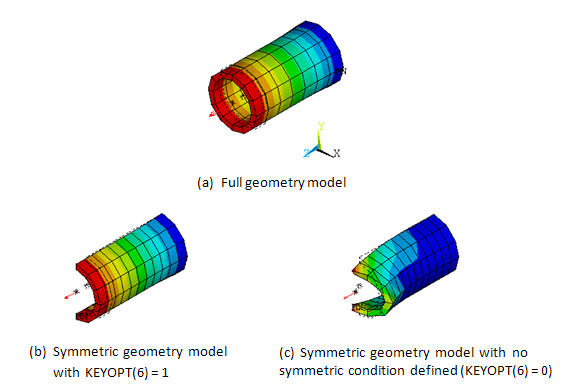
When the constrained surface is built on a symmetric geometry model instead of the full geometry model (for example, a symmetric boundary, a cyclic symmetry model , or a multistage cyclic symmetry model), you must define the symmetry conditions using KEYOPT(6) of the target element (TARGE169 or TARGE170). Otherwise, you might get unexpected results (as shown by (c) in Figure 10.12: Defining Symmetry Conditions for Force-Distributed Constraints). When defining symmetric conditions, the pilot node must be located on the symmetry plane/edge.
By default, the program computes weighting factors automatically by summing the contact area of each contact node. When you set KEYOPT(7) = 1 on the target element (TARGE169 or TARGE170), the program uses a constant weighting factor of 1.0 for each contact node (similar to the default behavior of RBE3). Alternatively, you can specify user-defined weighting factors by setting KEYOPT(7) = 2 and inputting a table of weighting factors for real constant FKN (similar to
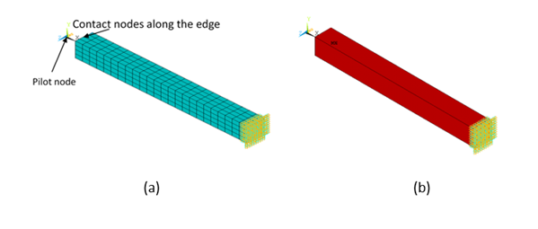
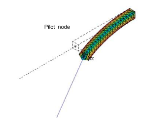
Wtfacton RBE3).When all the contact nodes are colinear (in a line), the moment along the colinear axis may not be transmitted. The program issues a warning message when this occurs. An example is presented in Figure 10.13: Colinear Contact Nodes with Force-Distributed Constraint - Solid Model. In the figure, (a) shows a moment applied on the pilot node that is parallel to the colinear axis (Z) in an attempt to bend the solid beam. Because of colinearity, the moment on the pilot node cannot be transmitted. Therefore, the solid beam remains undeformed as shown in (b) of the figure.
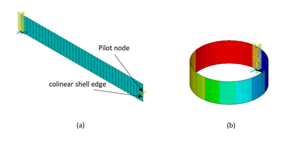
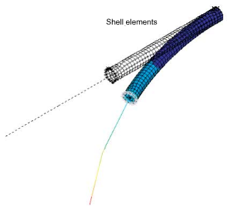
However, if the elements underlying the colinear contact nodes have rotation degrees of freedom, the program builds constraints on those DOFs. Figure 10.14: Colinear Contact Nodes with Force-Distributed Constraint - Shell Model demonstrates this case: a rotational 360 degree displacement is applied at the pilot node as show by (a). Force-distributed constraints are built along the edge of the shell tip. In contrast to the first example, the shell is bent the full 360 degrees as shown in (b) of the figure.
Another consequence of contact node colinearity in this type of constraint is that zero frequencies may occur in modal analysis, representing certain unconstrained rotational DOFs.
Restrictions for Force-Distributed Constraints Based on the Lagrange Multiplier Method
When a force-distributed constraint is defined with the Lagrange multiplier method (KEYOPT(2) = 3), the following restrictions apply:
Only structural degrees of freedom are supported.
Controlling the degrees of freedom with KEYOPT(4) of the target element is not supported.
Restrictions for Force-Distributed Constraints that Include Stress-Stiffening Effects
Force-distributed constraints based on the Lagrange multiplier method (KEYOPT(2) = 3) automatically include stress-stiffening effects. Force-distributed constraints based on the MPC approach (KEYOPT(2) = 2) include stress-stiffening effects if you set KEYOPT(10) = 1 on the target element. For both of these cases, the following restrictions apply:
The total number of nodes of a single force-distributed constraint cannot exceed 7,500.
A defined contact or target element type (ET) cannot be used in multiple contact pairs.
The pilot node is an independent (retained) node in the constraint equation. The contact nodes are the dependent (removed) nodes. Use caution when applying displacement constraints, coupling (CP), or constraint equations (CE) on the contact nodes, as redundant constraints are likely to occur.
KEYOPT(4) of TARGE169 and TARGE170 controls the DOF set (the number of DOF) of the contact (dependent) nodes used in the internally-generated MPCs.
The number of internally-generated MPCs is equal to the number of contact nodes times the number of DOF (when KEYOPT(2) = 2).
When the constrained surface is built on a cyclic symmetry model or multistage cyclic symmetry model, you must define the symmetry condition by setting KEYOPT(6) = 2 for the target element (TARGE169 or TARGE170). When defining symmetric conditions, the pilot node must be located on the symmetry plane/edge.
The contact surface does not require underlying elements.
A rigid surface constraint can undergo thermal expansion when KEYOPT(12) = 1 on the target element. You must also provide the value of the thermal expansion coefficient via the command MP,ALPX. Each contact node expands along the line that connects it to the pilot node. The temperature difference is evaluated as the average difference of the two nodes between the current and reference value. The thermal strain is calculated as logarithmic strain (NLGEOM,ON) or engineering strain (NLGEOM,OFF). However, the thermal strain is not an output quantity for the contact or target element.
To reduce result file size, report displacements only (zeroing out rotations) for free rigid body nodes (nodes that have no boundary conditions or connection to other elements).
Restrictions for Rigid Surface Constraints Based on the Lagrange Multiplier Method
When a rigid surface constraint is defined with the Lagrange multiplier method (KEYOPT(2) = 3), the following restrictions apply:
Only structural degrees of freedom are supported.
Controlling the degrees of freedom with KEYOPT(4) of the target element is not supported.
The pilot node is an independent (retained) node in the constraint equation. The contact nodes are the dependent (removed) nodes. It is strongly recommended that you do not apply any displacement constraints, coupling (CP), or constraint equations (CE) on the contact nodes in the same DOF direction as the coupling constraint since redundant constraints are likely to occur.
KEYOPT(4) of TARGE169 and TARGE170 controls the DOF set (the number of DOF) of the pilot node (the independent DOF) used in the internally-generated MPCs.
The DOF set defined by KEYOPT(4) follows the nodal coordinate system of the pilot node. Each contact node can have its own nodal coordinate system, which does not affect the solution.
The number of internally-generated MPCs is equal to the number of contact nodes times the number of DOF.
The surface-based constraint technique can be used to apply transitions between solid and structure elements. For example, a beam element connected to the solid or shell element face. One beam end node must be the pilot node and the solid/shell nodes must be the contact nodes. The rigid surface constraint is generally well-suited for the solid beam to solid surface case (see Figure 10.15: Beam-Solid Assembly Defined by Rigid Surface Constraint), and the force-distributed constraint is well-suited for the flexible beam (such as a thin wall beam) to solid/shell surface case (see Figure 10.16: Beam-Solid Assembly Defined by Force-distributed Constraint).
Force-distributed constraint models force and moment balance between a pilot node and the centers of surface nodes. Because force-distributed constraint was originally introduced to describe force balance in a bolt pattern, each surface node can carry a weight.
Force moments on a pilot are equivalent to the moment at the center of the weight:


It is straightforward to obtain the equation in the form of displacement:


Where:
 is the weight at each surface node
 is the pilot node displacement vector
 is the pilot node rotation pseudo-vector
 is the distance vector between the surface node and the
weighted center,
is the distance vector between the surface node and the
weighted center, 
 is the distance vector between the surface node and the
weighted center,
is the distance vector between the surface node and the
weighted center, 
 is the weighted center,
 is the inertial tension,
Note that this balance is only valid in the small defection scenario using the RBE3 command. To maintain the objective, additional corrections have been implemented in Mechanical APDL.