In addition to scalar (single valued) parameters, you can define array (multiple valued) parameters. Mechanical APDL arrays can be:
1D (a single column)
2D (rows and columns)
3D (rows, columns, and planes)
4-D (rows, columns, planes, and books)
5-D (rows, columns, planes, books, and shelves)
Mechanical APDL provides three types of arrays:
- ARRAY
This type is similar to FORTRAN arrays and is the default array type when dimensioning arrays. As with FORTRAN arrays, the indices for rows, columns, and planes are sequential integer numbers beginning with one. Array elements can be either integers or real numbers.
- CHAR
This is a character array, with each element consisting of an alphanumeric value not exceeding eight characters. The indices for rows, columns, and planes are sequential integer numbers beginning with one.
- TABLE
This is a special type of numeric array which allows Mechanical APDL to calculate (through linear interpolation) values between these array elements explicitly defined in the array. Moreover, you can define the array indices for each row, column, and plane and these indices are real (not integer) numbers. Array elements can be either integers or real numbers. As we'll see in the later discussion on TABLE arrays, this capability provides a powerful method for describing mathematical functions.
- STRING
You can use the *DIM, STRING capability to enter character strings into your arrays. Index numbers for columns and planes are sequential values beginning with 1. Row indices are determined by the character position in the string. See the *DIM command for more information.
The following array parameter topics are available:
- 3.10.1. Array Parameter Basics
- 3.10.2. Array Parameter Examples
- 3.10.3. Tabular Input via Table Array Parameters
- 3.10.4. Defining and Listing Array Parameters
- 3.10.5. Specifying Array Element Values
- 3.10.6. Writing Data Files
- 3.10.7. Operations Among Array Parameters
- 3.10.8. Plotting Array Parameter Vectors
- 3.10.9. Modifying Curve Labels
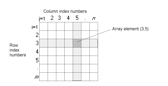
Consider a 2D array (either ARRAY or CHAR) as shown below. It is m rows long and n
columns wide; that is, its dimensions are m
times n. Each row is identified by a row index
number i, which varies from 1 to m, and each column is identified by a column index
number j, which varies from 1 to n. The quantities that make up the array are array
elements. Each array element is identified as (i,j), where i is its row
index number and j is its column index
number.
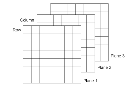
We can extend these definitions to a 3D array parameter, which may be
m rows long, n columns wide, and p planes deep. The
plane index number is k, which varies from 1 to
p. Each array element is identified as (i,j,k,). The following figure shows a 3D array.
Type ARRAY parameters consist of discrete numbers that are simply arranged in a tabular fashion for convenience. Consider the following examples.
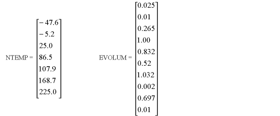

The parameter NTEMP could be an array of temperatures at selected nodes; NTEMP(1) = -47.6 could be the temperature at node 27, NTEMP(2) = -5.2 could be the temperature at node 43, and so on. Similarly, EVOLUM could be an array of element volumes, and COMPSTRS could be an array of nodal component stresses, with each column representing a particular direction (X, Y, Z, XY, YZ, XZ, for example).
A type CHAR array parameter is structured similarly to an ARRAY parameter, with the tabular values being alphanumeric character strings (up to eight characters). Two examples of character array parameters are:

A type TABLE array parameter consists of numbers arranged in a tabular fashion, much like the ARRAY type but with three important differences:
Mechanical APDL can calculate (via linear interpolation) any values that fall between the explicitly declared array element values.
A table array contains a 0 row and 0 column used for data-access index values and, unlike standard arrays, these index values can be real numbers.
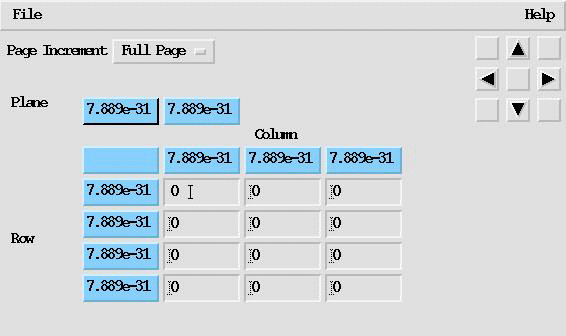
The only restriction is that the index values must consist of numerically increasing (never decreasing) numbers. You must explicitly declare a data access index value for each row and column; otherwise the default value assigned is the tiny number (7.888609052E-31). You can more conveniently define the index starting point and index values (*TAXIS).
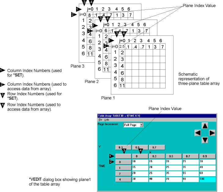
A plane index value resides in the 0,0 location for each plane.
The following figure shows a table array with data-access index values. The indices are specified as the "0" row and column values.
As shown in the above example, when configuring a table array you must set
The plane index value as the 0,0 element value for each plane.
The data-access column index values in the elements in the 0 row in plane 1. Only the column index values from plane 1 are used when accessing data from the array for all planes. When setting the array element values, you use the traditional row and column index numbers.
The data-access row index values in the elements in the 0 column in plane 1. Only the row index values from plane 1 are used when accessing data from the array for all planes. When setting the array element values, you use the traditional row and column index numbers.
For more information, see Defining Linear Material Properties Using Tabular Input in the Material Reference and Applying Loads Using Tabular Input in the Basic Analysis Guide.
To define an array parameter, first declare its type and dimensions (*DIM).
This following examples illustrate the *DIM command used to dimension various types of arrays:
*DIM,AA,,4  ! Type ARRAY is default, dimension 4[x1x1]
*DIM,XYZ,ARRAY,12       ! Type ARRAY array, dimension 12[x1x1]
*DIM,FORCE,TABLE,5      ! Type TABLE array, dimension 5[x1x1]
*DIM,T2,,4,3            ! Dimensions are 4x3[x1]
*DIM,CPARR1,CHAR,5      ! Type CHAR array, dimension 5[x1x1]
Note: Array elements for ARRAY and TABLE are initialized to 0 (except for the 0 row and column for TABLE, which is initialized to the tiny value). Array elements for CHAR are initialized to a blank value.
For array parameter operations (for example *VOPER, *VFUN), the resulting array parameter (ParR) need not be dimensioned beforehand. Also, array parameters defined completely with the implied (colon) loops convention (for example a(1:5)=10,20,30,40,50) need not be dimensioned beforehand.
The next example shows how to fill a 5-D array with data. Use 1D tables to load a 5-D table. Use the *TAXIS to define the table index values. See the full example at Example Analysis Using 5-D Table Array.
*dim,xval,array,X1
*dim,yval,array,Y1
yval(1)=0,20
*dim,zval,array,10
zval(1)=10,20,30,40,50,60,70,80,90,100
*dim,tval,array,5
tval(1)=1,.90,.80,.70,.60
*dim,tevl,array,5
tevl(1)=1,1.20,1.30,1.60,1.80

*dim,ccc,tab5,X1,Y1,Z1,D4,D5,X,Y,Z,TIME,TEMP
*taxis,ccc(1,1,1,1,1),1,0,wid                   !!! X-Dim
*taxis,ccc(1,1,1,1,1),2,0,hth                   !!! Y-Dim
*taxis,ccc(1,1,1,1,1),3,1,2,3,4,5,6,7,8,9,10    !!! Z-Dim
*taxis,ccc(1,1,1,1,1),4,0,10,20,30,40	           !!! Time
*taxis,ccc(1,1,1,1,1),5,0,50,100,150,200        !!! Temp
*do,ii,1,2
   *do,jj,1,2
      *do,kk,1,10
         *do,ll,1,5
            *do,mm,1,5
               ccc(ii,jj,kk,ll,mm)=(xval(ii)+yval(jj)+zval(kk))*tval(ll)*tevl(mm)
            *enddo
         *enddo
      *enddo
   *enddo
*enddo
You can specify array element values by
Setting individual array element values through the *SET command or "=" shortcut.
Filling individual vectors (columns) in the array with either specified or calculated values (the *VFILL command, for example).
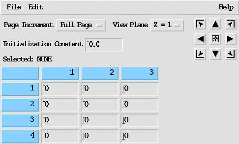
Interactively specifying values for the elements through the *VEDIT dialog.
Reading the values from an ASCII file (*VREAD or *TREAD commands).
Note: You cannot create or edit 4- or 5-D arrays interactively. *VEDIT, *VREAD, and *TREAD are not applicable to 4- or 5-D arrays.
You can use either the *SET command or the "=" shortcut. Usage is the same as for scalar parameters, except that you now define a column of data (up to ten array element values per "=" command). For example, to define the parameter XYZ dimensioned above as a 12x1 array you need two "=" commands. In the following example the first command defines the first eight array elements and the second command defines the next four array elements:
XYZ(1)=59.5,42.494,-9.01,-8.98,-8.98,9.01,-30.6,51
XYZ(9)=-51.9,14.88,10.8,-10.8
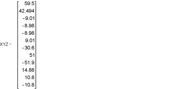
Notice that the starting location of the array element is indicated by the row index number of the parameter (1 in the first command, 9 in the second command).
The following example shows how to define the element values for the 4x3 array parameter T2, dimensioned earlier in the *DIM examples:
T2(1,1)=.6,2,-1.8,4           ! defines (1,1),(2,1),(3,1),(4,1)
T2(1,2)=7,5,9.1,62.5          ! defines (1,2),(2,2),(3,2),(4,2)
T2(1,3)=2E-4,-3.5,22,.01      ! defines (1,3),(2,3),(3,3),(4,3)

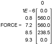
The following example defines element values for the TABLE array parameter FORCE discussed earlier.
FORCE(1)=0,560,560,238.5,0
FORCE(1,0)=1E-6,.8,7.2,8.5,9.3
The first "=" command defines the five array elements of the TABLE array FORCE. The second and third "=" commands redefine the index numbers in the j=0 and i=0 row.
Character array parameters can also be defined using the "=" command. Assigned values can be up to eight characters each and must be enclosed in single quotes. For example:
*DIM,RESULT,CHAR,3       !Character array parameter with dimensions (3,1,1)
RESULT(1)='SX','SY','SZ'  !Assigns values to parameter RESULT
Notice that, as when defining a numerical array parameter, the starting location of the array element must be specified (in this case, the row index number 1 is indicated).
You can use the *VFILL command to "fill" an ARRAY or TABLE vector (column).
See the *VFILL command reference information in the Command Reference for more detail about the command syntax. The following example illustrates the capabilities of the *VFILL command.
*DIM,DTAB,ARRAY,4,3                     ! dimension 4 x 3 numeric array
*VFILL,DTAB(1,1),DATA,-3,8,-12,57       ! four data values loaded into vector 1
*VFILL,DTAB(1,2),RAMP,2.54,2.54         ! fill vector 2 with values starting at
                                        ! 2.54 and incrementing by 2.54
*VFILL,DTAB(1,3),RAND,1.5,10            ! fill vector 3 with random numbers between
                                        ! 1.5 and 10.  Results vary due to
                                        ! random number generation.

The *VEDIT command, available only in interactive mode, launches a data entry dialog enabling you to edit an ARRAY or TABLE (not CHAR) array. The dialog provides a number of convenient features:
A spreadsheet-style editor for array element values.
Navigational controls for scrolling through large arrays.
An initialize function to set any row or column to a specified value (ARRAY type only).
Delete, copy, and insert functions for moving rows or columns of data (ARRAY type only).
Complete instructions for using the dialog are available from the box's Help button.
Note: You cannot edit a 4- or 5-D ARRAY or TABLE interactively.
You can fill an array from a data file via the *VREAD command. The command reads information from an ASCII data file and begins writing it into the array, starting with the index location that you specify. You can control the format of the information read from the file through data descriptors. The data descriptors must be enclosed in parenthesis and placed on the line following the *VREAD command. See Vector Operations for more information about data descriptors. The data descriptors control the number of fields to be read from each record, the width of the data fields, and the position of the decimal point in the field.
For example, given the following data file named dataval:
1.5     7.8  12.3
15.6  -45.6  42.5
and an array called EXAMPLE that has been dimensioned as 2 x 3, the following commands (provided as either a part or a macro or input listing)
*DIM,EXAMPLE,,2,3
*VREAD,EXAMPLE(1,1),dataval,,,JIK,3,2
(3F6.1)
result in
| EXAMPLE = |
1.5 7.8 12.3 15.6 -45.6 42.5 |
The *VREAD command cannot be issued directly from the command input window. However, the dialog offers a way to specify the data descriptors and issue the command in interactive mode.
Once configured, you have two options for specifying values for the TABLE array elements: you can add values as you would for any other type of array, or you can read in a table of data from an external file.
To read in a table of data from an external file, you still define the TABLE array first, specifying the number of rows, columns, and planes, and the labels for each. You can then read an ASCII file containing the table of data via the *TREAD command. At this time, you also specify the number of lines to skip (NSKIP) between the top of the file and the first line of the table.
When reading data from an external file, remember:
The file containing the table of data can be created in a text editor or an external application (such as Microsoft Excel), but it must be in ASCII form, tab-delimited, to be read into Mechanical APDL.
You must first define the array in Mechanical APDL, remembering to allow for the index values (0,0).
The values are read straight across the rows until all columns on each row of the array are filled; Mechanical APDL then wraps from one row to the next and begins to fill those columns, and so on. Be sure that the dimensions of the array you defined are correct. If you mistakenly define fewer columns in the Mechanical APDL array than required, Mechanical APDL begins filling in the next row of the array using the values remaining in the first row of the data table being read. Similarly, if you define more columns in the Mechanical APDL array than required, Mechanical APDL fills all columns of the array using values from the next row of the data table being read, and only then wrap and begin filling the next row.
You can create 1D, 2D, and 3D tables by reading data from an external file. Examples of how you create each of these follows.
Example 1: 1D Table
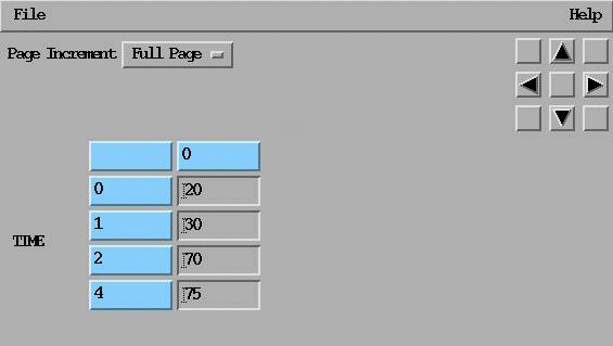
First, create the 1D table using the application of your choice (such as a spreadsheet application, a text editor, etc.) and then save the file as a text file in tab-delimited format. In this example, the table is named "Tdata" and contains data for a time vs. temperature table . In its ASCII form, the table would look like this:
Define a TABLE parameter "Tt" via the *DIM command. Specify four rows and one column, row label of Time, and column label of Temp. The data table you created has four rows and one column of data, plus the row and column index values (where the first column, TIME, is the row index values). Then, read in the file, specifying two skipped lines. The TABLE array in Mechanical APDL looks like this:
The same example using command input looks like this:
*DIM,Tt,table,4,1,1,TIME
*TREAD,Tt,tdata,txt,,2
Example 2: 2D Table
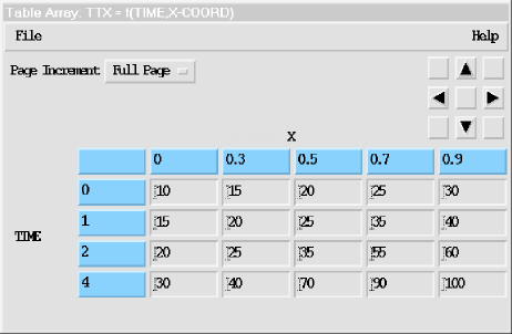
For this example, create (in a spreadsheet application, a text editor, etc.) a 2D table named "T2data" containing temperature data as a function of time and x-coordinate and read it into a TABLE array parameter called "Ttx." The table, in its ASCII form, would look like this:
In Mechanical APDL, you define a TABLE parameter "Ttx" using the *DIM command. Specify four rows, five columns, one plane, row label of TIME, and column label of X. The data table you created has four rows and five columns of data, plus the row and column index values. Then, read in the file, specifying two skipped lines. The TABLE array in Mechanical APDL looks like this:
The same example using command input looks like this:
*DIM,Ttx,table,4,5,,time,X
*TREAD,Ttx,t2data,txt,,2
Example 3: 3D Table
For this example, create a 3D table named "T3data" containing temperature data as a function of time, x-coordinate, and y-coordinate and read it into a TABLE array parameter called "Ttxy." The table, in its ASCII form, would look like this:
| Temp (time-X-coord) Table | |||||
|---|---|---|---|---|---|
| Time | X-Coordinate | ||||
| 0 | 0 | .3 | .5 | .7 | .9 |
| 0 | 10 | 15 | 20 | 25 | 30 |
| 1 | 15 | 20 | 25 | 35 | 40 |
| 2 | 20 | 25 | 35 | 55 | 60 |
| 4 | 30 | 40 | 70 | 90 | 100 |
| 1.5 | 0 | .3 | .5 | .7 | .9 |
| 0 | 20 | 25 | 30 | 35 | 40 |
| 1 | 25 | 30 | 35 | 45 | 50 |
| 2 | 30 | 35 | 45 | 65 | 70 |
| 4 | 40 | 50 | 80 | 100 | 120 |
In the example above, the bold values (in the (0,0,Z) positions) indicate the separate planes. Each plane of data, along with the row and column index values, is repeated for the separate planes. Only the plane index value and the actual data values are different. The shaded area above shows the values that change from plane to plane.
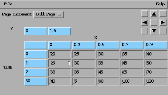
In Mechanical APDL, define a TABLE parameter "Ttxy" via the *DIM command. In the case of a 3D table, the table is dimensioned according to the number of rows, columns, and planes of data. The first column (TIME) is the row index values and the first row is the column index values. Specify four rows, five columns, two planes, row label of TIME, column label of X, and plane label of Y. The data table you created has four rows and five columns of data in two planes, plus the row and column index values. Then, read in the file, specifying two skipped lines. The TABLE array in Mechanical APDL looks like this for the second plane of data (Y=1.5):
The same example using command input looks like this:
*DIM,Ttxy,table,4,5,2,TIME,X,Y
*TREAD,Ttxy,t3data,txt,,2
When accessing information from the array, Mechanical APDL interpolates values between those explicitly set.
As examples of how Mechanical APDL interpolates values in TABLE arrays, consider the following:

Given that A is a TABLE array parameter, the Mechanical APDL program can calculate any value between A(1) and A(2), for example
A(1.5) evaluates to 20.0 (halfway between 12.0 and 28.0)
A(1.75) evaluates to 24.0
A(1.9) evaluates to 26.4
Similarly, if PQ is a TABLE array parameter
PQ(1.5,1) evaluates to -3.4 (halfway between 2.8 and -9.6)
PQ(1,1.5) evaluates to 3.5 (halfway between 2.8 and 4.2)
PQ(3.5,1.3) evaluates to 14.88
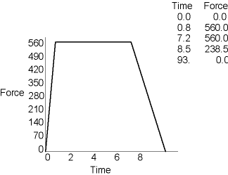
This feature allows you to describe a function, such as y=f(x), using a TABLE array parameter. You would use the j=0 column for values of the independent variable x and the "regular" j=1 column for values of y. Consider, for example, a time-history forcing function described by five points as shown below.
You can specify this function as a TABLE array parameter whose array elements are the force values, and whose row index numbers 1 through 5 are time values 0.0 through 9.3. Schematically, the parameter then looks like this:

Mechanical APDL can calculate (through linear interpolation) force values at times not specified in the FORCE parameter. For the above example, Mechanical APDL calculates a value of 89.4375 for FORCE(9). If a parameter location beyond the dimensions of the array is used, no extrapolation is done and the end value is used. For example, Mechanical APDL provides a value of 560.0 for FORCE(5,2) or 0.0 for FORCE(12)
You can see from these examples that TABLE array parameters can be very powerful tools in your analysis. Typical applications are time-history loading functions, response spectrum curves, stress-strain curves, material-versus- temperature curves, B-H curves for magnetic materials, and so forth. Be aware that TABLE array parameters require more computer time to process than the ARRAY type.
You can issue the *VGET command, which is similar to *GET, to retrieve Mechanical APDL-provided values and store them in an array.
You must define a starting array location number for the array parameter the *VGET command creates. Looping continues over successive entity numbers for the KLOOP default. For example, *VGET,A(1),ELEM,5,CENT,X returns the centroid x-location of element 5 and stores the result in the first location of A. Retrieving continues with elements 6, 7, and so on until successive array locations are filled. In this example, if KLOOP is 4, then the centroid of x, y, and z are returned.
To restore array parameter values, use the *VPUT command.
The *VPUT command uses the same arguments as the *VGET command (described above), but does the opposite of the *VGET operation. For a list of valid labels for *VPUT items, see the command's description in the Command Reference.
The Mechanical APDL program "puts" vector items directly, without any coordinate system transformation. *VPUT can replace existing array items, but can't create new items. Degree of freedom results that are changed in the database are available for all subsequent operations. Other results change temporarily, and are available mainly for immediately following print and display operations.
As with scalar parameters, you can use the *STATUS command to list array parameters. The following examples illustrate the *STATUS command in use:
*STATUS
 ABBREVIATION STATUS-

  ABBREV    STRING
  SAVE_DB   SAVE
  RESUM_DB  RESUME
  QUIT      Fnc_/EXIT
  POWRGRPH  Fnc_/GRAPHICS
  Mechanical APDLWEB  Fnc_HomePage

 PARAMETER STATUS-           (   5 PARAMETERS DEFINED)
                  (INCLUDING     2 INTERNAL PARAMETERS)

  NAME         VALUE         TYPE     DIMENSIONS
  MYCHAR      hi        CHARACTER
  MYPAR                     ARRAY       4       6       1
  MYPAR1    .987350000      SCALAR
*STATUS,XYZ(1),5,9      ! Lists rows 5 through 9 of XYZ
 PARAMETER STATUS- XYZ       (   4 PARAMETERS DEFINED)
      LOCATION          VALUE
      5     1     1   -8.98000000
      6     1     1    9.01000000
      7     1     1   -30.6000000
      8     1     1    51.0000000
      9     1     1   -51.9000000
*STATUS,FORCE(1),,,0 ! Lists parameter FORCE, includes j=0 column
PARAMETER STATUS- FORCE ( 4 PARAMETERS DEFINED)
      LOCATION          VALUE
      1     0     1   0.000000000E+00
      2     0     1   0.800000000
      3     0     1    7.20000000
      4     0     1    8.50000000
      5     0     1    9.30000000
      1     1     1   0.000000000E+00
      2     1     1    560.000000
      3     1     1    560.000000
      4     1     1    238.500000
      5     1     1   0.000000000E+00
*STATUS,T2(1,1) ! Lists parameter T2
PARAMETER STATUS- T2 ( 4 PARAMETERS DEFINED)
      LOCATION          VALUE
      1     1     1   0.600000000
      2     1     1    2.00000000
      3     1     1   -1.80000000
      4     1     1    4.00000000
      1     2     1    7.00000000
      2     2     1    5.00000000
      3     2     1    9.10000000
      4     2     1    62.5000000
      1     3     1   2.000000000E-04
      2     3     1   -3.50000000
      3     3     1    22.0000000
      4     3     1   1.000000000E-02
*STATUS,RESULT(1)!Lists parameter RESULT
PARAMETER STATUS- RESULT ( 4 PARAMETERS DEFINED)
LOCATION     VALUE
1     1     1     SX(CHAR)
2     1     1     SY(CHAR)
3     1     1     SZ(CHAR)
You can write formatted data files (tabular formatting) from data held in arrays through the *VWRITE command. The command takes up to 10 array vectors as arguments and writes the data contained in those vectors to the currently open file (*CFOPEN command). The format for each vector is specified with FORTRAN data descriptors on the line following the *VWRITE command (therefore you can't issue the *VWRITE command from the Mechanical APDL input window.)
An array vector, specified with a starting element location (such as MYARRAY(1,2,1)). You can also use an expression, which is evaluated as a constant value for that field in each row of the data file. The keyword SEQU evaluates to a sequential column of integers, starting from one.
The format of each row in the data file is determined by the data descriptor line. You must include one descriptor for each argument to the command. Do not include the word FORMAT in the descriptor line. You can use any real format or character format descriptor; however, you may not use either integer or list directed descriptors.
If you are unfamiliar with FORTRAN data descriptors, this section helps you to format your data file. For more information, consult the documentation for the FORTRAN compiler for your specific platform.
You must provide a data descriptor for each data item you specify as an argument to the *VWRITE command. In general, you can use the F descriptor (floating point) for any numeric values. The F descriptor takes the syntax
Fw.d
where
- w
Is the width of the data field in characters.
- d
Is the number of digits to the right of the decimal point.
Thus, for a field that is 10 characters wide and has eight characters after the decimal point, you would use the following data descriptor:
F10.8
For character fields, you can use the A descriptor. The A descriptor has the syntax
Aw
where
- w
Is the width of the data field in characters.
Thus, for a character field that is eight characters wide, the descriptor is
A8
The following examples illustrate the *VWRITE command and data descriptors in use.
Given that the MYDATA array has been dimensioned and filled with the following values:

The following short macro first defines the scalar parameter X as having a value of 25 and then opens the file vector (*CFOPEN command). The *VWRITE command then defines the data to be written to the file. In this case, the first vector written uses the SEQU keyword to provide row numbers. Note that in some cases that constants, scalar parameters, and operations that include array element values are written to the file. Note the data file contents for these items.
x=25
*cfopen,vector
*vwrite,SEQU,mydata(1,1,1),mydata(1,2,1),mydata(1,3,1),10.2,x,mydata(1,1,1)+3
(F3.0,'  ',F8.4,'  ',F8.1,'  'F8.6,'  ',F4.1,'  'F4.0,'  'F8.1)
*cfclos
The macro creates the following data file:
 1.    2.1522       3.9  5.286370  10.2   25.       5.2
 2.    2.3049       4.0  5.409196  10.2   25.       5.2
 3.    2.0105       3.4  5.936638  10.2   25.       5.2
 4.    2.3683       3.3  5.632203  10.2   25.       5.2
 5.    2.8491       4.8  5.978024  10.2   25.       5.2
 6.    2.2280       3.5  5.546851  10.2   25.       5.2
The second example uses the following previously dimensioned and filled array:

Note the use of descriptors in the following example *VWRITE command:
*vwrite,SEQU,mydata(1,1),mydata(1,2),(mydata(1,1)+mydata(1,2))
(' Row',F3.0,' contains ',2F7.3,'. Is their sum ',F7.3,' ?')
The resulting data file is
Row 1. contains  10.000 50.000.    Is their sum  60.000 ?
Row 2. contains  20.000 70.000.    Is their sum  60.000 ?
Row 3. contains  30.000 80.000.    Is their sum  60.000 ?
Just as parametric expressions and functions allow operations among scalar parameters, a series of commands is available to perform operations among array parameters. There are classes of operations: operations on columns (vectors), known as vector operations and operations on entire matrices (arrays), known as matrix operations. All operations are affected by a set of specification commands, which are discussed in Specification Commands for Vector and Matrix Operations.
Vector operations are simply a set of operations - addition, subtraction, sine, cosine, dot product, cross product, etc. - repeated over a sequence of array elements. Do-loops (discussed in Looping: Do-Loops) can be employed for this purpose, but a more convenient and much faster way is to use the vector operation commands - *VOPER, *VFUN, *VSCFUN, *VITRP, *VFILL, *VREAD, and *VGET. Of these listed vector operation commands, only *VREAD and *VWRITE are valid for character array parameters. Other vector operation commands apply only to array parameters dimensioned (*DIM) as ARRAY type or TABLE type.
The *VFILL, *VREAD, *VGET, *VWRITE, and *DIM commands were introduced earlier in this chapter. Other commands that are discussed in this section include
- *VOPER
Performs an operation on two input array vectors and produces a single output array vector.
- *VFUN
Performs a function on a single input array vector and produces a single output array vector.
- *VSCFUN
Determines the properties of a single input array vector and places the result in a specified scalar parameter.
- *VITRP
Forms an array parameter (type ARRAY) by interpolating an array parameter (type TABLE) at specified table index locations.
The examples below illustrate the use of some of these commands. Refer to the Command Reference for syntactical information about these commands. For all of the following examples, the array parameters (of type ARRAY) X, Y, and THETA have been dimensioned and defined.
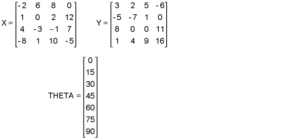
In the following example, the result array is first dimensioned (Z1). The *VOPER command then adds column 2 of X to column 1 of Y, both starting at row 1, and then places the result into Z1. Notice that the starting location (the row and column index numbers) must be specified for all array parameters. The operation then progresses sequentially down the specified vector.
*DIM,Z1,ARRAY,4
*VOPER,Z1(1),X(1,2),ADD,Y(1,1)

In the following example, again the result array (Z2) is dimensioned first. The *VOPER command then multiplies the first column of X (starting at row 2) with the fourth column of Y (starting at row 1) and writes the results to Z2 (starting at row 1).
*DIM,Z2,ARRAY,3
*VOPER,Z2(1),X(2,1),MULT,Y(1,4)

In this example, again the results array (Z4) is dimensioned first. The *VOPER command then performs the cross product of four pairs of vectors, one pair for each row of X and Y. The i, j, and k components of these vectors are columns 1, 2, and 3 respectively of X and columns 2, 3, and 4 of Y. The results are written to Z4, whose i, j, and k components are vectors 1, 2, and 3 respectively.
*DIM,Z4,ARRAY,4,3
*VOPER,Z4(1,1),X(1,1),CROSS,Y(1,2)

In the following example, the results array (A3) is dimensioned first. The *VFUN command then raises each element in vector 2 of X to the power of 2 and writes the results to A3.
*DIM,A3,ARRAY,4
*VFUN,A3(1),PWR,X(1,2),2

In this example, the results array (A4) is dimensioned. The two *VFUN commands then calculate the cosine and sine of array elements in THETA and place the results in the first and second columns, respectively, of A4. Notice that A4 now represents a circular arc spanning 90°, described by seven points (whose x, y, and z global Cartesian coordinates are the three vectors). The arc has a radius of 1.0 and lies parallel to the x-y plane at z = 2.0.
*DIM,A4,ARRAY,7,3
*AFUN,DEG
*VFUN,A4(1,1),COS,THETA(1)
*VFUN,A4(1,2),SIN,THETA(1)
A4(1,3)=2,2,2,2,2,2,2
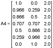
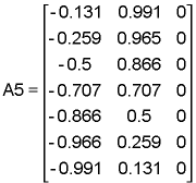
In this example, the results array (A5) is first dimensioned. Then, the *VFUN command calculates the tangent vector at each point on the curve represented by A4, normalizes it to 1.0, and places the results in A5.
*DIM,A5,ARRAY,7,3
*VFUN,A5(1,1),TANG,A4(1,1)
Two additional *VOPER operations, gather (GATH) and scatter (SCAT), are used to copy values from one vector to another based on numbers contained in a "position" vector. The following example demonstrates the gather operation. Note that, as always, the results array must be dimensioned first. In the example, the gather operation copies the value of B1 to B3 (using the index positions specified in B2). Note that the last element in B3 is 0 as this is its initialized value.
*DIM,B1,,4
*DIM,B2,,3
*DIM,B3,,4
B1(1)=10,20,30,40
B2(1)=2,4,1
*VOPER,B3(1),B1(1),GATH,B2(1)

Matrix operations are mathematical operations between numerical array parameter matrices, such as matrix multiplication, calculating the transpose, and solving simultaneous equations.
Commands discussed in this section include
- *MOPER
Performs matrix operations on one or more input array parameter matrices and produces an output array parameter matrix. Some of the available matrix operations are:
Matrix multiplication
Solution of simultaneous equations
Sorting (in ascending order) on a specified vector in a matrix
Covariance between two vectors
Correlation between two vectors
See *MOPER for a complete list of operations.
The examples below illustrate the use of some of these commands. Refer to the Command Reference for syntactical information about these commands.
This example shows the sorting capabilities of the *MOPER command. For this example, assume that the array (SORTDATA) has been dimensioned and its element values have been defined as follows:
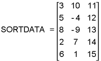
First, the OLDORDER array is dimensioned. The *MOPER command places the original order of the rows into OLDORDER. The *MOPER command then sorts the rows in SORTDATA so that the 1,1 vector is now in ascending order.
*dim,oldorder,,5
*moper,oldorder(1),sortdata(1,1),sort,sortdata(1,1)
The following array values result from the *MOPER command:

To put the SORTDATA array back into its original order, you could then issue the following command:
*moper,oldorder(1),sortdata(1,1),sort,oldorder(1,1)
In the following example, the *MOPER command solves a set of simultaneous equations. The following two arrays have been dimensioned and their values assigned:

The *MOPER command can solve a set of simultaneous equations for a square matrix. The equations take the form
an1X1 + an2X2 + , . . . , + annXn = bn
In the case of the above arrays, the *MOPER command solves the following set of simultaneous equations:
2X1 + 4X2 + 3X3 +2X4 = 2
3X1 + 6X2 + 5X3 + 2X4 = 2
2X1 + 5X2 + 2X3 - 3X4 =3
4X1 + 5X2 +14X3 + 14X4 = 11
To solve the equations, first the results array (C) is dimensioned. Then the *MOPER command solves the equations, using A as the matrix of a coefficients and B as a vector of b values.
*DIM,C,,4
*MOPER,C(1),A(1,1),SOLV,B(1)
The C array now contains the following solutions.

The following example shows the *MFUN command used to transpose data in an array. For this example, assume that the array (DATA) was dimensioned and filled with the following values:

As always, the results array (DATATRAN) is dimensioned first, then the *MFUN command transposes the values and writes them to DATATRAN.
*DIM,DATATRAN,,2,3
*MFUN,DATATRAN(1,1),TRAN,DATA(1,1)
The following shows the results in the DATATRAN array:

Vector and matrix operation commands are affected by the setting of the following array-specification commands: *VCUM, *VABS, *VFACT, *VLEN, *VCOL, and*VMASK. See the table below for details.
Of these commands, only *VLEN and *VMASK, in conjunction with *VREAD or *VWRITE, are valid for character array parameters.
You can check the status of these commands with the *VSTAT command.
Important: All specification commands are reset to their default settings after each vector or matrix operation.
Following are descriptions of the array-specification commands:
- *VCUM
Specifies whether results are cumulative or noncumulative (overwriting previous results). ParR, the result of a vector operation, is either added to an existing parameter of the same name or overwritten. The default is noncumulative results, that is, ParR overwrites an existing parameter of the same name.
- *VABS
Applies an absolute value to any or all of the parameters involved in a vector operation. The default is to use the real (algebraic) value.
- *VFACT
Applies a scale factor to any or all of the parameters involved in a vector operation. The default scale factor is 1.0 (full value).
- *VCOL
Specifies the number of columns in matrix operations. The default is to fill all locations of the result array from the specified starting location.
- *VSTAT
Lists the current specifications for the array parameters.
- *VLEN
Specifies the number of rows to be used in array parameter operations.
- *VMASK
Specifies an array parameter as a masking vector.
The following table lists the various specification commands and the vector and matrix array commands that they affect.
| *VABS | *VFACT | *VCUM | *VCOL | *VLEN ,NROW,NINC | *VMASK | ||
|---|---|---|---|---|---|---|---|
| *MFOURI | No | No | No | No | No | No | No |
| *MFUN | Yes | Yes | Yes | Yes | Yes | No | No |
| *MOPER | Yes | Yes | Yes | Yes | Yes | No | No |
| *VFILL | Yes | Yes | Yes | N/A | Yes | Yes | Yes |
| *VFUN | Yes | Yes | Yes | N/A | Yes | Yes | Yes |
| *VGET | Yes | Yes | Yes | N/A | Yes | Yes | Yes |
| *VITRP | Yes | Yes | Yes | N/A | Yes | Yes | Yes |
| *VOPER | Yes | Yes | Yes | N/A | Yes | Yes | Yes |
| *VPLOT | No | No | N/A | N/A | Yes | Yes | Yes |
| *VPUT | Yes | Yes | No | N/A | Yes | Yes | Yes |
| *VREAD | Yes | Yes | Yes | N/A | Yes | Yes | Yes |
| *VSCFUN | Yes | Yes | Yes | N/A | Yes | Yes | Yes |
| *VWRITE | No | No | N/A | N/A | Yes | Yes | Yes |
The examples below illustrate the use of some of the specification commands. Refer to the Command Reference for syntactical information about these commands.
In the following, the results array (CMPR) is dimensioned. The two *VFUN commands, in conjunction with the preceding *VMASK and *VLEN commands, then compress selected data and write them to specified locations in CMPR. The complement to the COMP operation is the EXPA operation on the *VFUN command.
*DIM,CMPR,ARRAY,4,4
*VLEN,4,2! Do next *V---- operation on four rows,
! skipping every second row
*VFUN,CMPR(1,2),COMP,Y(1,1)
*VMASK,X(1,3)!Use column 3 of X as a mask for next *V----
! operation
*VFUN,CMPR(1,3),COMP,Y(1,2)

This example uses the *VFACT command to round the values in an array vector to the number of decimal places specified by the NUMDP scalar parameter (set to 2 in the example). The NUMDATA array has been dimensioned and filled with the following values:

numdp=2
*vfact,10**numdp
*vfun,numdata(1),copy,numdata(1)
*vfun,numdata(1),nint,numdata(1)
*vfact,10**(-numdp)
*vfun,numdata(1),copy,numdata(1)
or, you can use a slightly shorter version
numdp=2
*vfact,10**numdp
*vfun,numdata(1),copy,numdata(1)
*vfact,10**(-numdp)
*vfun,numdata(1),nint,numdata(1)
The resultant NUMDATA array is then:

This example uses the *VLEN and *VMASK commands to find the set of prime numbers less than 100. An array, MASKVECT, is created using 1.0 to indicate that the row value is a prime number and 0.0 to indicate that the value isn't prime. The algorithm used to create the mask vector is to initialize all rows whose value is greater than 1 to 1.0 and then loop through the range of possible factors, eliminating all multiples of the factor. The *VLEN command sets the row increment for performing operations to FACTOR. When the *VFILL command is processed, the row number is incremented by this value. Because the starting row is FACTOR x 2, the rows are processed by each loop in the following manner: FACTOR x 2, FACTOR x 3, FACTOR x 4, etc.
*dim,maskvect,,100
*vfill,maskvect(2),ramp,1
*do,factor,2,10,1
*vlen,,factor
*vfill,maskvect(factor*2),ramp,0
*enddo
*vmask,maskvect(1)
*dim,numbers,,100
*vfill,numbers(1),ramp,1,1
*status,numbers(1),1,10
The resultant output from the *STATUS command, showing the first 10 elements in NUMBERS is:
PARAMETER STATUS- NUMBERS   (   5 PARAMETERS DEFINED)
                  (INCLUDING     2 INTERNAL PARAMETERS)

      LOCATION          VALUE
      1     1     1   0.000000000E+00
      2     1     1   2.00000000
      3     1     1   3.00000000
      4     1     1   0.000000000E+00
      5     1     1   5.00000000
      6     1     1   0.000000000E+00
      7     1     1   7.00000000
      8     1     1   0.000000000E+00
      9     1     1   0.000000000E+00
10 1 1 0.000000000E+00You can graphically display array vector values using the *VPLOT command.
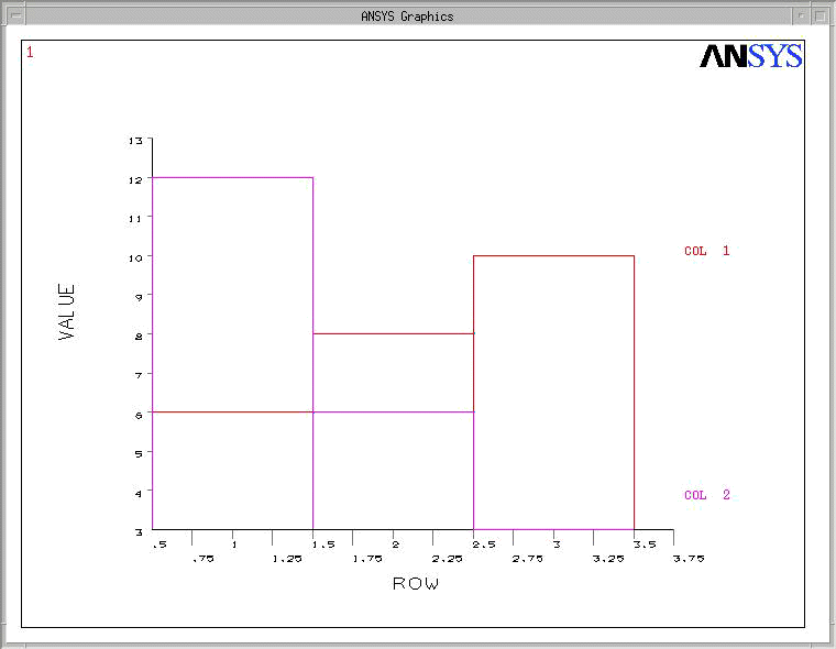
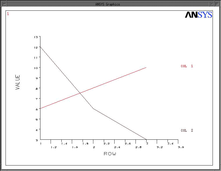
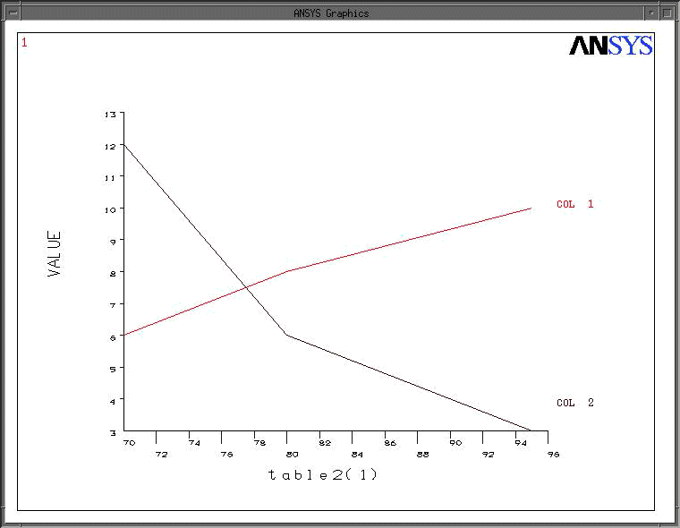
The following demonstrates some of the capabilities of the *VPLOT command. For this example, two TABLE arrays (TABLEVAL and TABLE) and one numeric array have been dimensioned and filled with the following values:
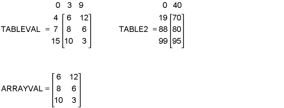
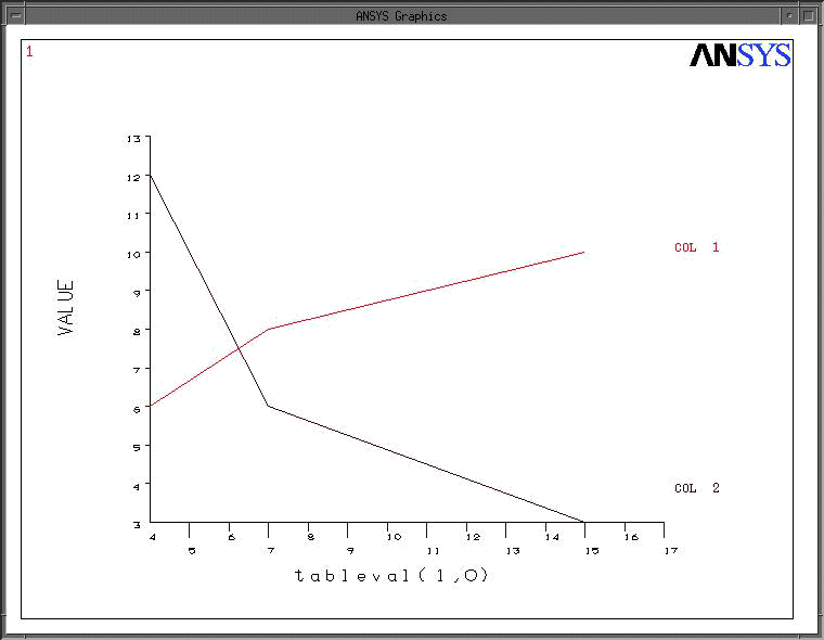
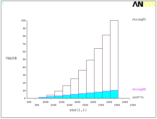
The following are example *VPLOT commands and their resulting plots. Note that since ARRAY data is unordered it is plotted as a histogram; TABLE data is ordered and is therefore plotted as a curve.
When you use *VPLOT to create your curves, default labels are assigned. Normally, the label for curve 1 is "COL 1", the label for curve 2 is "COL 2" and so on; the column number is the field containing the dependent variables for that particular curve. You can use the /GCOLUMN command to apply your own labels to the curves (any string of up to eight characters).
The example below uses the /GCOLUMN command at the beginning of the program input to apply the labels "string01" and "string02" to the array curve.
/gcol,1,string01
/gcol,2,string02

*dim,xxx,array,10
*dim,yyy,array,10,2

xxx( 1,1) =1e6
xxx( 2,1) = 1e6 + 1e5
xxx( 3,1) = 1e6 + 2e5
xxx( 4,1) = 1e6 + 3e5
xxx( 5,1) = 1e6 + 4e5
xxx( 6,1) = 1e6 + 5e5
xxx( 7,1) = 1e6 + 6e5
xxx( 8,1) = 1e6 + 7e5
xxx( 9,1) = 1e6 + 8e5
xxx(10,1) = 1e6 + 9e5

yyy( 1,1) = 1
yyy( 2,1) = 4
yyy( 3,1) = 9
yyy( 4,1) = 16
yyy( 5,1) = 25
yyy( 6,1) = 36
yyy( 7,1) = 49
yyy( 8,1) = 64
yyy( 9,1) = 81
yyy(10,1) = 100

yyy( 1,2) = 1
yyy( 2,2) = 2
yyy( 3,2) = 3
yyy( 4,2) = 4
yyy( 5,2) = 5
yyy( 6,2) = 6
yyy( 7,2) = 7
yyy( 8,2) = 8
yyy( 9,2) = 9
yyy(10,2) = 10

*vplo,xxx(1,1), yyy(1,1) ,2
The labels can be returned to the default value (COL 1 and COL 2) by issuing the /GCOLUMN command with no string specified.
/gcol,1
/gcol,2


