


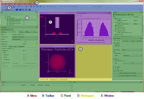
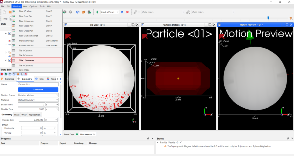
Ansys Rocky software is a powerful program with a flexible, hierarchical interface. One main screen gives you access to the most frequently used functions and features, and provides you with various views of the simulation.
Additional panels allow you to access properties and settings to fine-tune your simulation and view statistics based upon the results.
What would you like to learn about?
See Also:
Use this section to explore the five major parts of the Rocky user interface, and learn when and why you might access them.
What would you like to do?
Learn more About the Menu
Learn more About the Toolbar
Learn more About Panels
Learn more About Workspaces
See Also:
The menu is always located at the very top of the Rocky main screen and is one of the few UI elements in Rocky that is static in its location. From the Rocky menu, you can do all of the following tasks:
From the File menu:
Begin a new simulation project (see also Begin a New Simulation Project).
Open an existing simulation project (see also Open an Existing Simulation Project).
Save a new simulation project (see also Save a New Simulation Project).
Archive a simulation project (see also Archive a Simulation Project).
Restore an archived project (see also Restore an Archived Simulation Project).
Export or import project context (see also Reuse 3D View Window, Workspace, and User Process Setups in Other Projects).
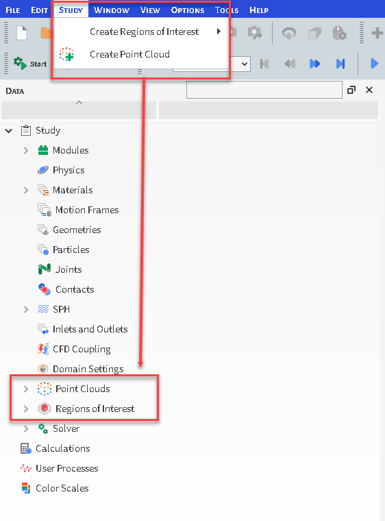
From the Study menu:
Create Regions of Interest.
Create Point Cloud.
From the Edit menu:
Undo or Redo actions made in Rocky (see also About the Undo/Redo History Panel).
Copy an Image or Data Set to the clipboard (see also Copy an Image or Data Set to the Clipboard).
From the Window menu, you can create, organize (see also Edit or Remove a Workspace), and save an image of (see also Save an Image of the 3D View, Plot, or Histogram) various Rocky windows, including:
3D View windows (see also Create and Modify a 3D View).
Plot and Histogram windows (see also Graphing (Plot or Histogram) a Data Set Within Rocky).
Motion Preview windows (see also Preview a Motion in 3D).
Particles Details windows (see also Preview a Particle Shape in 3D).
From the View menu:
Show/hide various Rocky panels (see also About Panels).
Revert to the default Rocky user interface layout by clicking Reset layout.
Change the background color of the Rocky interface by selecting a Theme. In this version, there are two options:
Dark Theme,(default) which has a mostly black background with light-colored text.
Light Theme, which has a mostly white background with dark-colored text.
From the Options menu:
Set global preferences for using Rocky (see also About Setting Global Preferences).
Set the units used in Rocky (see also About Setting Your Unit System).
Install coupling components required for use with Ansys Fluent (see also Install Ansys Coupling Components).
From the Tools menu, you can show/hide all of the following panels:
The PrePost Script panel (see also About Creating and Using PrePost Scripts).
The Python Shell panel (see also Customize and Extend Rocky with Python).
The Inspection panel (see also About the Cell Inspector).
The Animation panel (see also About Creating and Saving an Animation).
The Expressions/Variables panel (see also Defining Your Variables).
From the Help menu, you can do all of the following:
Access your Rocky License status and info by clicking License Info.
Review details about this Rocky release by clicking About. (See also About This Version of Rocky.)
Access the User Manual (this document), DEM Technical Manual, and other resources by pointing to Manuals and then selecting which option you want. (See also Getting Help and Support.)
Access the Tutorials, Community forum and other features by pointing to Customer Portal and then selecting which item you want.
Review the technical library, the latest Rocky applications and other resources by pointing to Website and then clicking the option you want to access.
Learn about the key improvements made for this release of Rocky by clicking What's New.
Review what changed in this release of Rocky by clicking Release Notes.
Access the default Workspace that displays when you first open Rocky by clicking Start Page.
See Also:
The toolbar is, by default, located at the top of the Rocky main screen just below the menu. There are several individual toolbar components that can make up the main Rocky toolbar, including the following:
Camera visualization toolbar (see also About Using the Camera Visualization Toolbar)
Coloring service toolbar (see also About Using the Coloring Service Toolbar to Change a 3D View)
Custom Presets toolbar (see also About the Custom Presets Toolbar)
File toolbar
Time toolbar (see also About the Time Toolbar)
Undo Redo toolbar
These individual toolbar components can be moved or made to float independent of the screen by clicking a toolbar handle and then dragging it and dropping it with the mouse. You can also show/hide individual toolbars by right clicking a toolbar and selecting or clearing the options at the very bottom of the contextual menu.
See Also:
Below the toolbar and surrounding the Workspace are various floating panels that enable you to set parameters and choose options for your simulation and its resulting data. The primary panels for configuring your simulation are the Data and Data Editors panels that appear (by default) to the left of the Workspace; the primary panels for post-processing are the Windows and Windows Editors panels that appear (by default) to the right of the Workspace. Also showing (by default) to the right of the Workspace, you can display various tools panels such as Animations or PrePost Script. You can choose to show/hide multiple panels through both the View and Tools menus located at the top of the screen.
All panels in Rocky can be resized, moved, nested with other panels, and undocked to float independent of the Rocky main screen. Specifically:
To resize a panel, hover your mouse over a panel boundary until the resize icon appears. Then, click and drag the boundary to the desired width or height.
To move a panel to another docked location, click the panel title and drag to the desired area outside of the Workspace. While still dragging the panel, a preview of new docked locations will be displayed with a blue background. To select a new docked location, release the mouse over the preview of the location you want.
To make a nested panel, click the panel title and then drag it directly over another panel until the lower panel is blue, and then release the mouse. The second panel will appear as a tab at the bottom of the first panel. Select the tab you want to toggle between panels.
To make a docked panel float, click the panel title, drag it towards the center of the screen then release the mouse. Alternatively, you can also click the icon to the left of the panel's close button to make any docked panel float.
Show/hide multiple panels by right clicking a panel's title bar and selecting or clearing the options at the top and middle of the contextual menu.
What would you like to do?
Learn more About the Data Panel
Learn more About the Data Editors Panel
Learn more About the Windows Panel
Learn more About the Window Editors Panel
Learn more About the Undo/Redo History Panel
Learn more About the Log Panel
Learn more About the Simulation Log Panel
Learn more About the Cache Panel
Learn more About the Debug Info Panel
Learn more About the Progress Panel
Learn more About the Status Panel
Learn more About the PrePost Script Panel
Learn more About the Inspector Panel
Learn more About the Animations Panel
Learn more About the Python Shell Panel
Learn more About the Expressions/Variables Panel
See Also:
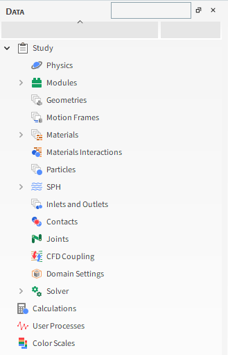
The Data panel is the area you use to select the entity with which you want to interact. The tree-like structure is hierarchical and is roughly organized by the steps required to setup, process, and analyze your project. (See Figure 1.)
By clicking Study on the menu, more parameters can be added to the Data Panel, as shown in the image below:
The top-level items in the Data panel include the following entities:
Study, which organizes all the various set-up and processing categories. (See also Set Simulation Parameters and Processing a Simulation.)
Calculations, which lists any Particles or SPH elements Properties you have applied to User Processes for which you want to retain calculations after the particle/SPH element leaves the defined area. (See also About Particles Calculations.)
User Processes, which lists the shapes, planes, and settings you have divided or filtered your simulation area into for more focused analysis. (See also Filter Views and Data with User Processes.)
Color Scales, which lists all the Properties you have shown in a 3D View for the purpose of changing the coloration of the legends. (See also Create and Modify a 3D View.)
Once selected in the Data panel, options for the item are generally shown in the Data Editors panel (see also About the Data Editors Panel), or through the item's right-click menu. Note: With the exception of the Study item, which has its own settings, top-level Data panel items are for categorization only and do not have settings associated with them. Only the sub-items listed beneath these categories will have settings upon which you can take action.
The Data panel also includes a search box to help you find items in the panel quickly. (See also Use the Data Panel Search Bar to Quickly Find Components.) You may also duplicate many of the items in the Data panel to save time on setup. (See also Duplicate a Data Panel Item.)
See Also:
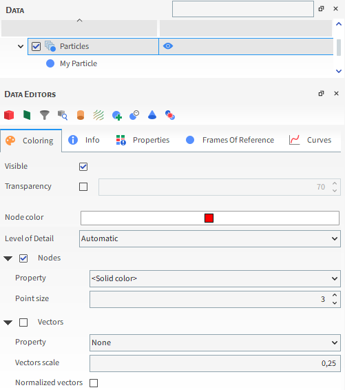
The Data Editors panel shows the settings and parameters available for the item selected in the Data panel (see also About the Data Panel). Figure 1 shows the Data Editors panel view when Particles is chosen in the Data panel.
What is shown for an entity on the Data Editors panel can include action buttons, like those provided at the top of Figure 1, and settings and information organized into various tabs, such as the following:
Coloring tab (see also About the Coloring Tab)
Info tab (see also About the Info Tab)
Properties tab (see also About Properties)
Curves tab (see also About Curves)
Some entities in the Data panel, such as Particles Calculations and Color Scales, are categories only and will have no information displayed in the Data Editors panel. However, sub-items within these categories will have information upon which you can take action.
See Also:
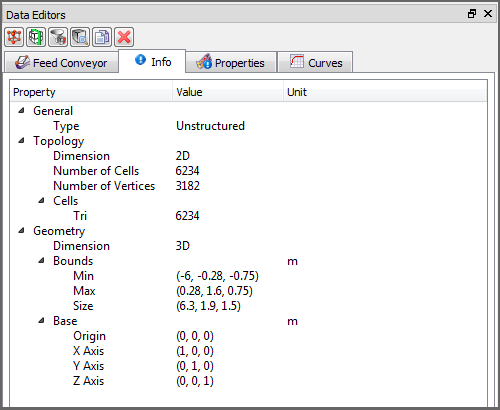
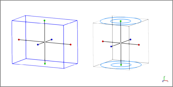
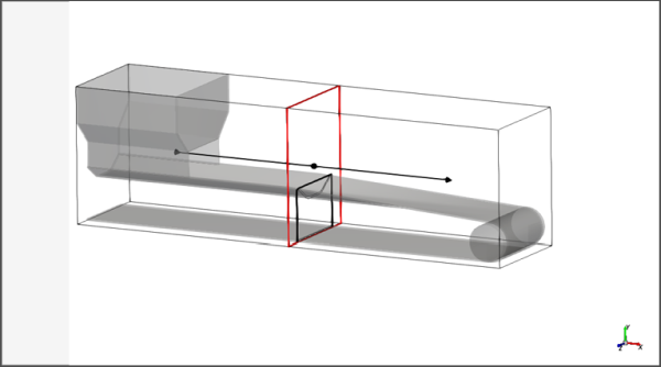
The Info tab is one of several tabs that appear on the Data Editors panel when a simulation entity is selected in the Data panel. Though purely informational, the Info tab does show some data about the selected entity that could be useful when setting up or analyzing your simulation.
For example, the Info tab can display domain properties, such as the topology and geometry coordinate limits, that provide context as to how the Property simulation data was recorded. These properties are displayed on the Info tab for simulation entities including conveyors (Figure 1) and imported geometries, the main Particles entity, 1-Way LBM, 1-Way Fluent, and individual User Processes.
ABOUT THE INFO TAB FOR MODULES
The Info tab on individual Modules (see also About Modules Parameters) describes the Author and Version details for the Module, and lists what other entities in the Rocky UI are affected by enabling that particular Module. For example, the Info tab for the Liquid Bridge Model Module (Figure 2) describes three places in the Rocky UI affected by that module.
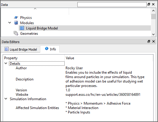
Note: In this version of Rocky, the Liquid Bridge Model Module is provided as an external module. Refer to the Install an External Module topic for details.
This information can help you verify that the parameters in those locations are set correctly for the feature enabled by the module.
ABOUT THE INFO TAB FOR INDIVIDUAL PARTICLE SETS
When an individual Particle set is selected under the main Particles entity, the Info tab shows useful information about the largest particle in the selected particle set, but also contains additional functionality unique to that tab (Figure 3).
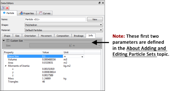
For example, you can change the units by clicking a unit and selecting a new type from the list that appears. You can also use the Custom Size (Custom Diameter or Custom Scale Factor) checkbox to experiment with different particle sizes and how they affect the properties displayed on the Info tab without having to switch back to the Size tab. Note: This functionality is explained in more detail in the About Adding and Editing Particle Sets topic.
ABOUT THE MAX ADMISSIBLE OVERLAP VALUE(for Custom Concave Particles)
The Max Admissible Overlap value is provided only for custom (imported) concave particles. Its purpose is to display the maximum percentage of concave overlap that will be allowed during the simulation.
As a comparison, for a sphere and a boundary collision, the maximum overlap allowed is 50%— above that the sphere center would be on the other side of the boundary and the particle would cross it. For concave particles, the maximum admissible overlap depends on the shape. Ideally, the maximum admissible overlap should not be too low, or you will have to compensate for that by using a larger Young's modulus for stability.
Tip: If you have imported a concave particle with values too small for the maximum overlap allowed, consider modifying the STL shape to result in higher values. This might help you avoid numerical issues.
Use the following information to help you better understand this value and how best to use it:
What is this value used for? It is a reference that can help you prevent excessive overlaps that can cause numerical instabilities for the concave particle shape used in the simulation. The smaller the maximum admissible overlap, the smaller are the overlap values that are tolerated during the simulation.
How is this value calculated? It is computed based upon the minimum distance from the particle's triangle centers to other triangles of the particle in the direction perpendicular to the triangle's plane. So the max admissible overlap is a function of the particle shape. Sharp edges will result in lower maximum admissible overlaps to guarantee the solver's stability.
How does this value relate to the STL file I imported? This is not a quality criteria for the STL file itself; rather, it is related to the particle shape. If the shape has more rounded or sharp edges, it will be reflected on the max admissible overlap value. So more (or fewer) overlaps will be admitted to ensure the stability of the simulations.
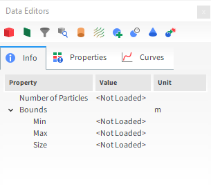
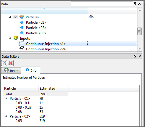
ABOUT THE INFO TAB FOR INPUT ENTITIES
For Inputs (Figure 4), the Info tab displays the simulation particle count in different ways depending upon the particle size distribution that was specified:
For Particle sets made up of only one size (no size distribution), the Info tab shows the exact number of particles that will be released into the simulation.
For Particle sets with a size distribution, the Info tab provides an estimate of the number of particles that could be released into the simulation.
Note: For Volume Fill specifically, the estimate assumes there are no boundary limits to consider, and assumes a Gap Scale Factor equal to 1. This means that if you have set your particle Mass higher than the box and gap you define can contain, the particle estimate on the Info tab will show a higher number than what will actually be injected.
For Particle sets with size ranges specified, viewing the Simulation Summary after processing has begun is still the only place to get an exact particle count; however, if a particle count estimate is sufficient, the particle count on the Input entity's Info tab can be viewed at any time during project setup. (See also About the Simulation Summary.)
See tables below to help you understand more about the Info tab.
Table 1: Info tab definitions for individual Geometry components, Inlets, the main Particles entity, 1-Way LBM, 1-Way Fluent, and individual User Processes (Figure 1 above)
Property | Description | Values Displayed |
|---|---|---|
General | ||
Type | Indicates the type of grid the domain property is based upon. Specifically:
| Unstructured; Structured |
Topology | ||
Dimension | Indicates whether the domain property has no dimension; or is one dimensional (node), two dimensional (triangle), or three dimensional (block or cell). | 0D; 1D; 2D; 3D |
Number of Cells | Lists the number of cell within the simulation bounds. | Positive whole numbers |
Number of Vertices | The number of cell intersections within the simulation bounds. For geometries, this is the points between triangle. For Eulerian Statistics, this is the corner points making up each block And so on. | Positive whole numbers |
Cells Point | For Particles, lists the number of points within the simulation bounds. | Positive whole numbers |
Cells Tri | For Geometry components, lists the number of triangles within the simulation bounds. | Positive whole numbers |
Cells Bar | For Particle Trajectory calculations, lists the total number of trajectory bars that were calculated. | Positive whole numbers |
Shape | For Eulerian Statistics, indicates the number of divisions that were defined in the X, Y, and Z directions respectively. | Whole values greater than or equal to 1 |
Geometry | ||
Dimension | Indicates whether the geometry components within the simulation have no dimension; or are one dimensional (node), two dimensional (triangle), or three dimensional (block or cell). | 0D; 1D; 2D; 3D |
Bounds Min | The minimum coordinates of the simulation data. | X, Y, Z |
Bounds Max | The maximum coordinates of the simulation data. | X, Y, Z |
Bounds Size | The size dimensions of the current simulation bounds. | X, Y, Z |
Length | For Particle Trajectory calculations, provides the total length of the trajectory lines added together. | Positive values |
Volume | For Eulerian Statistics, provides the total volume of all the Eulerian blocks added together. | Positive values |
Table 2: Info tab definitions for individual Modules (Figure 2 above) (See also About Modules Parameters.)
Property | Description | Values Displayed |
|---|---|---|
Details | ||
Author | If provided, lists the name of the developer or company that designed and built the Module. | Text |
Description | If provided, displays a short description of what the Module does. | Text |
Version | If provided, displays the Module version. For Modules created by Ansys, this will be equal to the version of Rocky for which the Module was designed. | Text |
Website | If provided, displays the URL of the website associated with the Author of the Module. | Text |
Simulation Information | ||
Affected Simulation Entities | Describes whether or not enabling the Module caused changes or additional settings to be made in other areas of the Rocky UI. Specifically:
| Text |
Table 3: Info tab definitions for individual Particle sets (Figure 3 above) (See also About Adding and Editing Particle Sets.)
Property | Description | Values Displayed |
|---|---|---|
Scale Factor | By default, when the Custom Scale Factor checkbox is cleared, this displays the size of the largest particle in the Particle set using the Original Size Scale method of measurement that was selected on the Size sub-tab. When the Custom Scale Factor checkbox is enabled, this displays the experimental size entered in the corresponding Scale Factor) box. (See also About Adding and Editing Particle Sets.) | Positive values |
Equivalent Diameter | By default, when the Custom Diameter checkbox is cleared, this displays the size of the largest particle in the Particle set using the Equivalent Sphere Diameter method of measurement that is selected on the Size sub-tab. When the Custom Diameter checkbox is enabled, this displays the experimental size entered in the corresponding Diameter box. (See also About Adding and Editing Particle Sets.) | Positive values |
Sieve size | By default, when the Custom Size (Custom Diameter or Custom Scale Factor) checkbox is cleared, no matter what is selected for Size Type on the Size sub-tab, this converts the size of the largest particle to its Sieve Size value, which is based upon the dimensions of a square hole just big enough for the particle to pass through. When the Custom Size (Custom Diameter or Custom Scale Factor) checkbox is enabled, this displays the experimental size entered in the corresponding Size (Diameter or Scale Factor) box converted into its Sieve Size value. (See also About Adding and Editing Particle Sets.) | Positive values |
Volume | By default, when the Custom Size (Custom Diameter or Custom Scale Factor) checkbox is cleared, this displays the volume of the largest particle in the Particle set. When the Custom Size (Custom Diameter or Custom Scale Factor) checkbox is enabled, this displays the volume of the experimental particle defined in the corresponding Size (Diameter or Scale Factor) box. (See also About Adding and Editing Particle Sets.) | Positive values |
Area | By default, when the Custom Size (Custom Diameter or Custom Scale Factor) checkbox is cleared, this displays the surface area of the largest particle in the Particle set. When the Custom Size (Custom Diameter or Custom Scale Factor) checkbox is enabled, this displays the surface area of the experimental particle defined in the corresponding Size (Diameter or Scale Factor) box. (See also About Adding and Editing Particle Sets.) | Positive values |
Moments of Inertia x | By default, when the Custom Size (Custom Diameter or Custom Scale Factor) checkbox is cleared, this displays the moment of inertia in the X direction of the largest particle in the Particle set. When the Custom Size (Custom Diameter or Custom Scale Factor) checkbox is enabled, this displays the moment of inertia in the X direction for the experimental particle defined in the corresponding Size (Diameter or Scale Factor) box. (See also About Adding and Editing Particle Sets.) | Positive values |
Moments of Inertia y | By default, when the Custom Size (Custom Diameter or Custom Scale Factor) checkbox is cleared, this displays the moment of inertia in the Y direction of the largest particle in the Particle set. When the Custom Size (Custom Diameter or Custom Scale Factor) checkbox is enabled, this displays the moment of inertia in the Y direction for the experimental particle defined in the corresponding Size (Diameter or Scale Factor) box. (See also About Adding and Editing Particle Sets.) | Positive values |
Moments of Inertia z | By default, when the Custom Size (Custom Diameter or Custom Scale Factor) checkbox is cleared, this displays the moment of inertia in the Z direction of the largest particle in the Particle set. When the Custom Size (Custom Diameter or Custom Scale Factor) checkbox is enabled, this displays the moment of inertia in the Z direction for the experimental particle defined in the corresponding Size (Diameter or Scale Factor) box. (See also About Adding and Editing Particle Sets.) | Positive values |
Mass | By default, when the Custom Size (Custom Diameter or Custom Scale Factor) checkbox is cleared, this displays the mass of the largest particle in the Particle set. When the Custom Size (Custom Diameter or Custom Scale Factor) checkbox is enabled, this displays the mass of the experimental particle defined in the corresponding Size (Diameter or Scale Factor) box. (See also About Adding and Editing Particle Sets.) | Positive values |
Elements | For Particle sets with Multiple Elements selected on the Composition sub-tab, this displays the number of individual element that the particle shape will be divided into. Specifically:
(See also About Adding and Editing Particle Sets.) | Positive values |
Triangles | By default, when the Custom Size (Custom Diameter or Custom Scale Factor) checkbox is cleared, this displays the number of triangles that make up the largest particle in the Particle set. When the Custom Size (Custom Diameter or Custom Scale Factor) checkbox is enabled, this displays the number of triangles making up the experimental particle defined in the corresponding Size (Diameter or Scale Factor) box. (See also About Adding and Editing Particle Sets.) Note: The way in which particle shape triangles are counted in Rocky depend upon the particle shape and composition. Specifically:
| Positive values |
Vertices | For Particle sets made up of custom (imported) particle shapes, this displays the number of points between the triangle (for Custom Shells or Custom Polyhedrons) or between the segments (for Custom Fibers) that make up the particle shape. Specifically:
(See also About Adding and Editing Particle Sets.) Note: The way in which vertices are counted in Rocky depend upon the particle shape that was imported. Specifically:
| Positive whole numbers |
Max Admissible Overlap | For custom imported concave particles, displays the maximum percentage of concave overlap that will be allowed during the simulation. | 0-100 |
Custom Shape Type | For custom shapes that are imported into Rocky from an .stl file, this displays the category to which Rocky has assigned the shape. Rocky categorizes shapes based upon various attributes and also uses those categories to determine what kind calculations to perform during processing. Tip: For more information about how Rocky categorizes custom particle shapes, refer to the DEM Technical Manual. (From the Rocky Help menu, point to Manuals, and then click DEM Technical Manual.) | Concave; Convex; Fiber; Not Custom; Shell |
Table 4: Info tab definitions for individual Particle Inputs (Figure 4 above) (See also About Adding and Editing Particle Inputs.)
Property | Description | Values Displayed |
|---|---|---|
Total | For the main Inputs entity, this displays the total amount of particles that are estimated to be released into the simulation from all individual Particle Inputs. For individual Particle Inputs (Figure 3), this displays the total amount of particles that are estimated to be released into the simulation from only that input. Note: For Particle sets with only one size specified, the particle count is exact. For Particle sets with a size distribution, the particle count is an estimate only. | Positive whole numbers |
<Particle Input Name> (automatically provided) | For the main Inputs entity, this displays the total amount of particles that are estimated to be released into the simulation from only the selected input. Note: For Particle sets with only one size specified, the particle count is exact. For Particle sets with a size distribution, the particle count is an estimate only. | Positive whole numbers |
<Particle Name> (automatically provided) | For each individual Particle Input listed on either the main Inputs entity or on its own Info tab (Figure 3), this displays the amount of particles from only this Particle set that are estimated to be released into the simulation from the input to which it is assigned. When expanded, the top most total amount is further broken down by the particle size ranges specified for the Particle set. Note: For Particle sets with only one size specified, the particle count is exact. For Particle sets with a size distribution, the particle count is an estimate only. | Positive whole numbers |
Tip: If you see <Not Loaded> listed for items under the Value column, right-click the item and then click Load… to have Rocky calculate and display the values.
See Also:
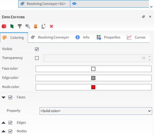
The Coloring tab, located on the Data Editors panel when a simulation entity is selected in the Data panel, helps you change the colors and data attributes of your selected entity.
The options displayed on the tab are dependent upon which type of window you select. If a 3D Plot window is selected, the Coloring tab shows options that enable you to change the appearance of the entity you have selected in the Data panel (Figure 1). Those changes will be visible in the 3D View.
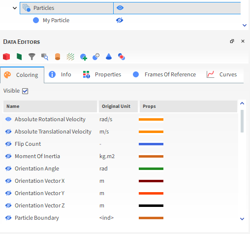
If a plot or histogram window is selected, the Coloring tab shows the data sets that are already calculated and ready to display in the window (Figure 2). The active data sets are indicated with an "open" eye icon. (See also Show/Hide Components by Using Eye Icons and Checkboxes.) Unlike when a 3D View window is selected, the data on the Coloring tab when a plot or histogram window is selected is not dependent upon what is selected in the Data panel.
If a Motion Preview window is selected, the Coloring tab shows options related to the axes of the Frame that is selected in the Data panel.
Figure 2.12: Coloring tab when a Motion Frame is selected in the Data panel AND a Motion Preview window is selected
If a Particles Details window is selected, the Coloring tab shows options that will enable you to change the appearance of the particle shape you have selected to display. You can also adjust the transparency settings, allowing you to finely tune the opacity of the particle and achive the desired level of transparency (Figure 4).

See Also:
The Windows panel enables you to easily view, create, or remove the various Rocky windows-including 3D View windows, Motion Preview windows, and plots and histogram windows-all in one place (Figure 1).
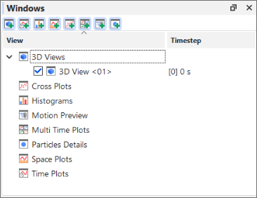
It is hidden by default when you first open Rocky, but can be shown by selecting Windows from the View menu.
On the Windows panel, existing windows are listed below their categories, and new windows can be created from the button bar at the top of the panel. And by using the checkboxes, windows can be shown or hidden from the workspace without actually removing them from the project. (See also Show/Hide Components by Using Eye icons and Checkboxes.)
Selecting a window from this panel will enable that window's editable properties in the Window Editors panel.
See Also:
The Window Editors panel (Figure 1) displays the editable settings and parameters for the Rocky window that is selected in the Windows panel (see also About the Windows Panel).
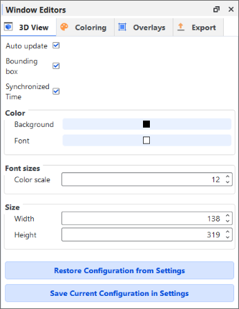
Depending upon the type of window that is selected, different options will be presented, such as the following:
Window-type-specific options, such as background color, and font sizes.
Coloring, which provides options for displaying the data (geometries, graph lines, etc.) shown in the selected window.
Overlays, which provides options for adding text or images to the 3D View window.
Export, which provides options for exporting and then viewing images or data from the window outside of Rocky.
See Also:
The Log panel is for more advanced users of Rocky. Its purpose is to display the actions you have taken in the program that Rocky records for bug reporting purposes (Figure 1). When an error is shown in the program, you are sometimes given the option of submitting a report with your feedback. That report would contain details regarding the actions displayed in this panel.
This kind of information can be useful when writing and testing scripts. (See also About Creating and Using PrePost Scripts.)
For example, the actions displayed on the Log panel can be referenced while playing a script (Figure 1), which can be useful for debugging purposes.
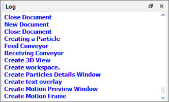 Figure 1: Log panel showing some actions that were recorded
In addition, if a print function is referenced when creating a script (Figure 2), it will appear in the Log panel when the script is played (Figure 3).
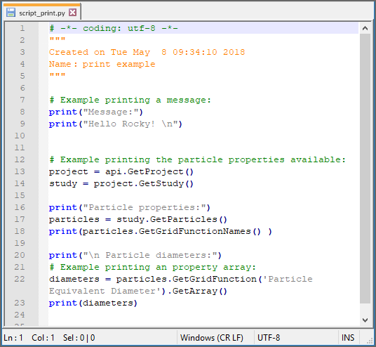 Figure 2: Example script making use of a print function
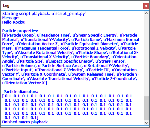 Figure 3: Log panel showing print function when example script is played
The Log is for display only and cannot be edited. Like the Undo/Redo history panel (see also About the Undo/Redo History Panel), the items displayed in this panel are cleared every time you close and open the project.
See Also:
The Simulation Log panel displays any solver-related warnings, errors, or other information that happen during processing (Figure 1), no matter whether you are running your simulations using CPU or GPU resources. This kind of information can be useful when troubleshooting issues that occur when you process your simulation project.
Figure 2.16: Simulation Log panel showing some warnings and information that was logged during processing
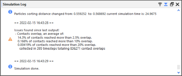
The Simulation Log is for display only and cannot be edited. But because it is possible to get many messages per simulation, you are able to filter the results and/or have Rocky automatically scroll to the bottom of the list by using the Filter and Auto Scroll buttons, respectively, at the top of the panel.
Unlike the other Log panels in Rocky, the items displayed in this panel are retained when the project is closed. This is to help you troubleshoot any issues with the Solver that might have caused Rocky to stop processing. It can also be useful in cases where you have used the Rocky Scheduler (see also About Processing Multiple Simulations In Succession) to process a project and want to review what errors or warnings were recorded by the solver during processing.
The Simulation Log is cleared whenever a new simulation or project is started.
Tip: For details about some of the more asked-about warnings and errors that can appear on your Simulation Log panel, see also I get warnings or errors on my Simulation Log Panel.
SIMULATION LOG PANEL FUNCTIONALITY
See the table below for information about the Simulation Log panel functionality.
Table 1: Simulation Log panel functionality
Button | Description | Range |
|---|---|---|
| Enables you to reduce the information shown to only messages of certain types. Messages are filtered by level of importance. Specifically:
Tip: To see all messages of any type, ensure that the Filter is set to Information. | Information; Warning; Error |
| Enables you to determine whether Rocky will automatically scroll the view area in the panel when new information is added, or will keep the view area stationary. Tip: To always see the latest messages without having to scroll down in the panel, ensure Auto Scroll is turned on. | Turns on or off |


See Also:
The Cache panel is for more advanced users of Rocky. It is designed to list the Rocky processes that take up memory (Figure 1), and also enables you to remove any unused processes that are no longer needed (Figure 2). This information can be used to optimize how Rocky uses the memory available.
Note: Memory allotment for Rocky is set from the Preferences dialog. (See also About Setting Global Preferences.)
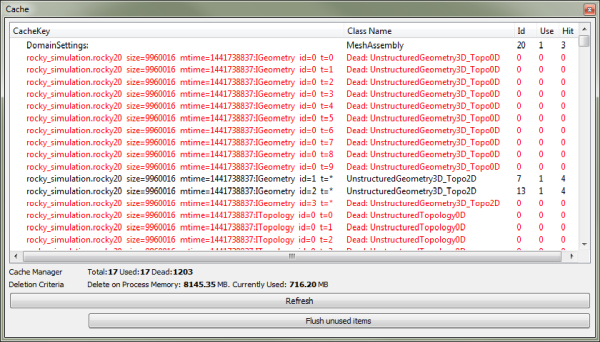
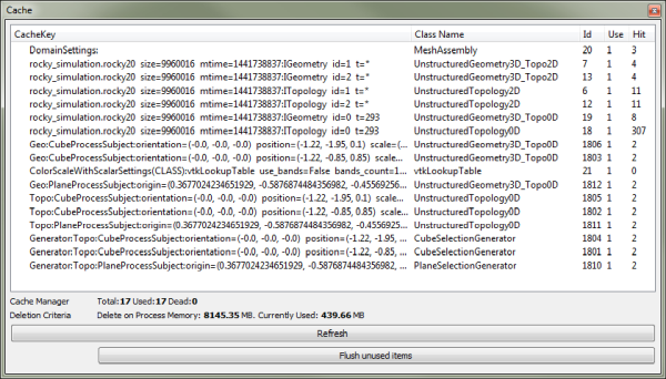
Use the table below and images above to help you understand more about the Cache panel.
Table 1: Cache panel settings
Setting | Description |
|---|---|
Cache list | Lists individual Rocky processes taking up memory. Tip: Click the Refresh button to view the current list. |
Cache Manager | Counts the processes in the Cache list and organizes them by the following criteria:
|
Deletion Criteria | Describes how processes will be deleted. Specifically:
|
See Also:
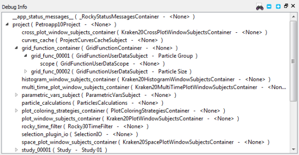
The Debug Info panel is for advanced users of Rocky. It is designed to list code-related items for the purpose of solving issues found within the program (Figure 1).
See Also:
The Undo/Redo history panel Figure 2.20: Undo/Redo history panel showing some example actions is one way you can review and undo the actions you took on your project. Each separate step you take or setting you change is chronologically listed in this panel. When you Undo or Redo an action- either by using the panel, the toolbar, or keyboard - the choices you make are reflected here. The last action applied to the project is marked with a blue arrow; active actions are listed in black; inactive (or "undone") actions are listed in gray Figure 2.21: Undo/Redo history panel showing some example actions that have been undone.
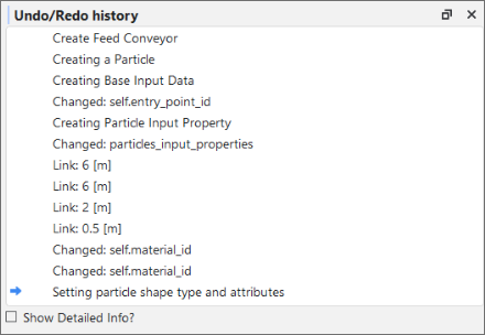

You can use the toolbar or keyboard to undo or redo one action at a time. You can use the panel to undo or redo every action up to the action you select. In this way, you can "undo" or "redo" as many actions as you like with only a double-click.
The actions listed in the panel are cleared every time you close and open the project.
What do you want to do?
UNDO OR REDO SEVERAL ACTIONS AT ONCE
Ensure the Undo/Redo history panel is open. (From the View menu, click Undo/Redo history.)
Do one of the following:
To undo several actions at once, find the blue arrow marking the current action, scroll up the list and then double-click the black-colored action to which you want to revert. The blue arrow now marks the action you selected and all later actions are colored gray to indicate that they are now inactive.
To redo several actions at once, find the blue arrow marking the current action, scroll down the list and then double-click the gray-colored action to which you want to redo. The blue arrow now marks the action you selected and all previous actions are colored black to indicate that they are now active.
See Also:
UNDO OR REDO A SINGLE ACTION AT ONCE
Do one of the following:
Click the Undo or Redo buttons on the toolbar.
Press Ctrl+Z or Ctrl+Y on your keyboard.
See Also:
A Workspace is a collection of Rocky windows. Located in the center of the Rocky screen, the windows that make up a Workspace are where you choose to view the physical components of your simulation setup (3D View windows), and interact with the graphical results of your simulation (plot and histogram windows).
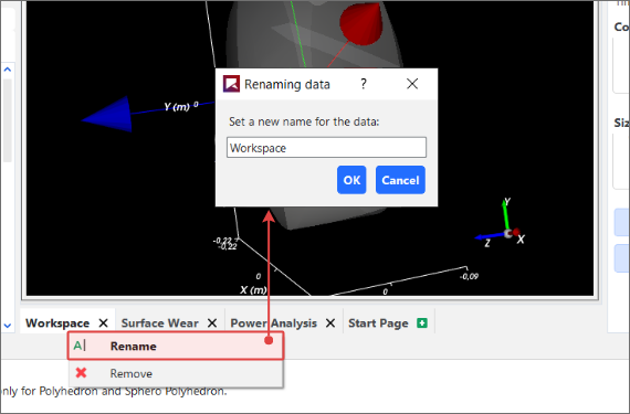
You can have multiple Workspaces for different purposes, such as by analysis type. These are designated by Workspace tabs along the bottom of the Workspace area Figure 2.22: Example tabs at the bottom of the Workspace area, which can also be renamed to help you better categorize your data Figure 2.23: Renaming a Workspace. You can also use the tiling options in the Windows menu to better organize your windows on the Workspace Figure 2.23: Renaming a Workspace.

What would you like to do?
See Also:
From the bottom of the center Workspace area, on the Start Page tab, click the green "+" icon. A new tab appears at the bottom of the Workspace.
Tips:
To change the name of the Workspace, right-click the Workspace tab and then in the Renaming data dialog, enter a new name and then click OK.
To add windows to the Workspace, see the following topics:
See Also:
Do one or more of the following:
To remove an existing Workspace, right-click tab for the Workspace you want to remove, and click the red "X" icon. Note: Removing the Workspace also removes any window(s) that you had placed on the Workspace. This can be reversed with the Undo function. (See also Undo or Redo a Single Action at Once.)
To add another Workspace, on the Start Page Workspace tab, click the green "+" icon.
To change the name of the Workspace, do the following:
Right-click the Workspace tab, and click Rename.
From the Renaming data dialog, enter a new name for the Workspace, and then click OK.
To arrange the windows orderly on a Workspace, from the Windows menu, select the Tile Columns option you want.
To add windows to the Workspace, see the following topics:
See Also:
This section covers the not-so-obvious but useful features scattered throughout the Rocky UI and how it might benefit you to use them.
What would you like to do?
See Input/Output Relationships in the Data Panel When Component Names are Bold
Determine the Frequency of Calculations by Pinning/Unpinning Items
Double-Click the Status Panel to Jump to the Appropriate UI Location
Refer to the Rocky Title Bar for Simulation Progress Details
Lock a Curve Selection to a Plot to Quickly Change the Data Shown
Double-Click a Plot Line, Bar, or Point to Change Its Appearance
See Also:
NAME COMPONENTS TO AFFECT SORT ORDER
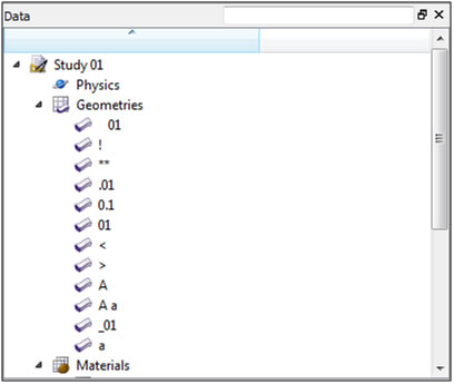
Sorting in Rocky follows the rules for Extended ASCII character codes (For a full list, see Appendix B: ASCII Printable Characters.) In general, Names beginning with spaces are sorted first, followed by most special characters, followed by numbers, followed by uppercase letters, and ending with lowercase letters.
For example, Rocky would sort the following 12 geometry components in the order shown in Figure 1.
See Also:
SHOW/HIDE COMPONENTS BY USING EYE INCONS AND CHECKBOXES
Rocky provides two complementary methods for determining whether a component or family of components will be shown or hidden in the Workspace: The eye icon (Figure 1), which affects the visibility of only that individual component, and the checkbox (Figure 2), which affects the visibility of all sub-components beneath the object.
![]() Figure 1 : Open and closed eye icons to the right of objects in the Data
panel
Figure 1 : Open and closed eye icons to the right of objects in the Data
panel
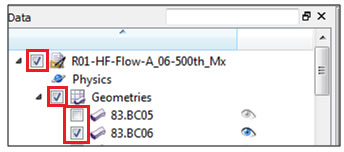 Figure 2 : Checkboxes to the left of objects in the Data panel
Eye Icon
An "open" eye icon (default setting) indicates that particular object is visible or shown in 3D View windows, plots, or histograms. A "closed" eye icon keeps that item in the simulation's calculations but makes the object appear invisible or hidden in the window. This is useful for seeing behind one object to another in an animation, for example, or for focusing on a particular curve in a plot.
Checkbox
In the Data panel, the checkbox has the same visibility affect as the eye icon but is hierarchical, meaning it affects all children components directly beneath that item in the Data panel. For example, clearing the checkbox to the left of Geometries hides all individual geometry components listed beneath it.
In the Windows panel, the checkbox acts like the eye icon does in the Data panel: it shows/hides the individual object—in this case, various windows in the Workspace. Unlike in the Data panel, checkboxes in the Windows panel are not hierarchical.
See Also:
SEE INPUT/OUTPUT RELATIONSHIPS IN THE DATA PANEL WHEN COMPONENT NAMES ARE BOLD
Linked objects refer to the ability of a geometry component, Particles, or 1-Way LBM to provide data to a particular User Process, thus establishing an input/output relationship between them. This linkage is illustrated in the Data panel by the name of the object providing the data (output) turning bold when the User Process that is accepting the data (input) is selected, as shown in Figure 1.
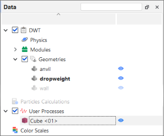 Figure 1 : Example of a geometry component shown in bold when the user
process linked to it is selected
Figure 1 : Example of a geometry component shown in bold when the user
process linked to it is selected
To create this kind of input/output relationship, the User Process must be created directly from the object providing the data. In the example above, the Cube <01> user process was created by selecting the dropweight geometry and then creating a Cube user process from either the Data Editor or right-click menu.
See Also:
DETERMINE THE FREQUENCY OF CALCULATIONS BY PINNING/UNPINNING ITEMS
After processing your simulation, you can view various types of data on the Properties and Curves tabs for your simulation settings like particles and geometry components. Each of the items listed on these tabs has a pin icon to the left of it, as illustrated in Figure 1.
![]() Figure 1 : Pin icons on the Properties tab of the Data Editors panel
Figure 1 : Pin icons on the Properties tab of the Data Editors panel
The color of these pin icons indicates how often Rocky calculates the particular item, as follows
A gray-colored pin (default) indicates that the item will not be calculated for any output time. Choosing to avoid calculating data that you don't need saves processing time and power during your simulation
A red-colored pin indicates that the item will be calculated for each output time included in the simulation. And if settings affecting those values change, Rocky will recalculate to keep all the values current. Important: Choosing to have Rocky calculate the item at each output time is likely to take up a significant amount of processing time and power. Only choose to pin items for which having all output time calculations be kept up-to-date and available are truly necessary for your analysis.
Tip: To pin or unpin an item, just left-click the pin icon.
Alternately, you can choose to have Rocky calculate any values you are interested in once, by right-clicking the item and choosing Compute Statistics. (See also About Viewing an Individual Statistic.)
See Also:
Rocky uses several different characters and strings as placeholders for calculations or explanations that would take up too much room in the UI. Here is a quick list of some placeholders you might run across and what they mean.
Note: These placeholders might appear on the Info, Properties, or Curves tabs (Data Editors panel).
Placeholder | Description |
|---|---|
? | Information isn't calculated yet. Same as "Not loaded." |
Not loaded | Information isn't calculated yet. Same as "?". |
- | Item contains no unit for the value displayed. Generally indicates a ratio, such as a percentage. |
Unable to calculate | Not enough information available at this particular output time in order to calculate the values. |
Unknown | Not enough information is known to calculate the value. |
<ind> | Item contains no units for the value displayed. Generally indicates a index, such as a count or a coordinate position. |
-1.#IND | Calculation is invalid. This can happen to Particle properties, for example, if there are no particles in the simulation at the time specified for the calculation. |
N/A | Value is Not Applicable (N/A) to the selected item. |
See Also:
DOUBLE-CLICK THE STATUS PANEL TO JUMP TO THE APPROPRIATE UI LOCATION
If you have errors listed in the Status panel (Figure 1), you can double-click those errors to be taken to the location in the Data panel where you would address them.
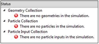
For example, if you double-click the "There are no geometries in the simulation" error, Rocky would enable the Geometries item in the Data panel.
See Also:
USE COLORED TEXT TO VALIDATE THE SYNTAX OF YOUR ENTRIES
Rocky provides instant feedback for entering functions and variables into a parameter text field by coloring the text as you type, as explained below:
Red text indicates that the syntax of the active entry is not yet valid. The syntax is based upon the rules of the Python programming language. It will tell you whether you have an open parenthesis that needs to be closed, for example.
Green text indicates that the syntax of the active entry is valid. Note: Green text does not indicate that the value, function, or variable of active entry has been formatted correctly or is itself a valid entry. Validation happens after either pressing Enter or clicking away from the text field.
Black text indicates a currently inactive entry.
See Also:
There are several tasks in Rocky that can be accomplished more easily by dragging items with your mouse and dropping them to another location, as described below:
Creating new views of Particles, individual geometry components, or Air Flow: From the Data panel, select the component(s) you want to view and then drag and drop them to a window of your choice (3D View, Histogram, or Time Plot). Only the component(s) you selected will be added.
Creating new views of data sets: From the Data Editors panel, on the Curve or Properties tab, select the data item(s) you want to show and then drag and drop them into the window type you want (3D View, plots or histograms).
Creating multiple Multi-Time plots in a single window: After adding your first data set, hold the Ctrl key while selecting your next data set and then drag and drop it into the gray area of an existing Multi-Time plot window. Another plot appears in the same window.
Tip: You can also multi-select items to drag and drop. (For example, show multiple geometry components at once in a 3D View.) Just hold the Ctrl or Shift key while left clicking your selections with the mouse, and then drag and drop as usual.
See Also:
ACCESS THE RIGHT-CLICK MENU FOR ADDITIONAL FEATURES
There are a few things in Rocky that can only be accomplished by right-clicking the item, as described below:
Adding/Importing geometry components: From the Data panel, right-click Geometries to access the menu that enables you to add or import new geometry components.
Computing statistics for only the current output time: From the Data Editors panel, on the Curves or Properties tab, right-click the data item you want to view values for and then click Compute Statistics from the right-click menu.
Showing only a few components in a new window: From the Data panel, select the item(s) you want displayed in a new window, right-click your selection, and then from the right-click menu, point to Show in New and then click the window type you want. Only the items you selected appear in the new window.
Import your own User Process shape for particle analysis: From the Data panel, right-click Particles, point to User Processes, and then click Polyhedron (Envelope). From the Select the STL file for the polyhedron dialog, navigate to the STL file you want, and then click Open. The polyhedron you chose appears under the User Processes list. Note: You can also create a custom-shaped User Process from any existing User Process that was originally created from a Particle set. (See also See Input/Output Relationships in the Data Panel When Component Names are Bold.) From the Data panel, under User Process, right-click a User Process that was created from a Particle set and then follow the instructions above.
See Also:
USE THE DATA PANEL SEARCH BAR TO QUICKLY FIND COMPONENTS
The search bar is located at the very top right of the Data panel, as shown in Figure 1.
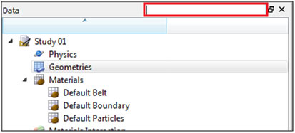 Figure 1 : Data panel search bar
When you start typing into it, Rocky immediately displays in the Data panel the entire hierarchy of the component(s) that best match what you typed. In a simulation setup with many different components, using the search bar can help you find what you need faster than scrolling.
Tips:
To search the names in order from left to right, enter the first few characters of the component you want to find. For example, to find all components that begin with "belt," type belt into the search box. You would find "belt 01" and "belt 02" but not "feeder belt" by using this method.
To search anywhere in the name, type an asterisk (*) followed by the characters anywhere within the name that you want to find. For example, to find all components containing "belt" anywhere in the name, type *belt into the search box. In this way, you would find the "feeder belt" component as well as "belt 01" and "belt 02."
See Also:
REFER TO THE ROCKY TITLE BAR FOR SIMULATION PROGRESS DETAILS
When you are actively processing a simulation (see also About Starting a Simulation), the Title bar for the Rocky program displays useful details about the simulation's progress. (Figure 1.)
 Figure 1 : Example of Title bar progress information shown while a
simulation is processing
Figure 1 : Example of Title bar progress information shown while a
simulation is processing
This progress information in the Title bar includes the following:
Output: The total number of output files that have been saved thus far. In the example in Figure 1, the total number of output files saved so far is 81.
Current progress: The particular second of the total Simulation Duration that Rocky is currently calculating. Note that Rocky calculates in finer detail than is typically determined by the Output Frequency in which it saves output files. In the example in Figure 1, although Rocky is currently calculating for second 4.050, because the simulation output frequency is set to 0.05 seconds, it won't actually save a 82nd output file representing 4.100 seconds until the current progress reaches that point.
Elapsed: Amount of real time since starting (or resuming) the simulation processing. In the example in Figure 1, 12 seconds have elapsed since the simulation was resumed.
ETA: Rocky's estimate of how much real time the simulation will take to complete. This is a rough approximation Rocky extrapolates based upon the amount of time the last several outputs took to calculate. In the example in Figure 1, Rocky estimates that it will take roughly 2 minutes and 49 seconds to complete. The ETA will get longer as more and more particles enter the simulation and it takes more time for Rocky to calculate each output. Should the simulation reach a point where more particles leave the simulation than enter it, the ETA will begin to get shorter. Once the simulation enters a steady state, this value will likely be a very good estimate of the remaining time.
See Also:
LOCK A CURVE SELECTION TO A PLOT TO QUICKLY CHANGE THE DATA SHOWN
If you want to see the same curve (for example, Particle Mass) in a plot (for example, Time Plot) across many similar Data panel elements (for example, several User Processes created from Particles), you can use the Replace Curves According to Data Tree Selection toggle button (Figure 1), which is available for any Time Plot, Multi Time Plot, or Cross Plot.
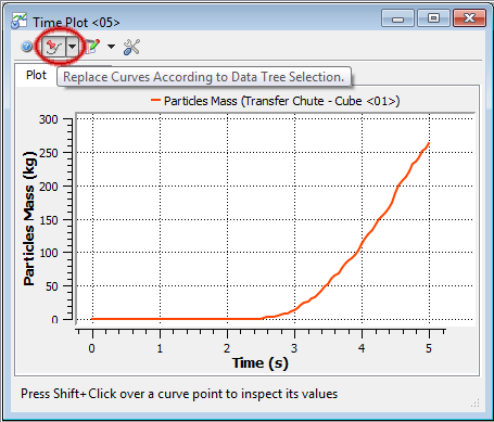
When you toggle (push in) this button on a plot you have created and then select another similar item on the Data panel, the curve you original selected stays the same but the data is replaced with the data corresponding to the item you just selected (Figure 2).
Figure 2.28: Original plot (top); second Data panel option selected with button toggled (middle); third Data panel option selected with button toggled (bottom)
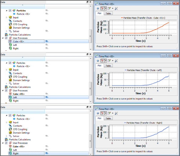
In this way, you can quickly compare the same curve across many similar Data panel items without having to create many separate plots. This button also works if you multi-select curves.
To turn off this feature, click the toggle button again to push it out.
See Also:
DOUBLE-CLICK A PLOT LINE, BAR, OR POINT TO CHANGE ITS APPEARANCE
Similar to the Edit Expression dialog that you get when you click the Edit Formula button on the Table tab of a Time Plot (see also About Time Plots), you can also change the Pen style, color, and width as well as the data point appearance by double-clicking the line, bar, or point in the plot or histogram. This will bring up the Edit Curves dialog (Figure 1) and from there, you can change the settings as you like.
Tip: You can also right-click the line, bar, or point and then from the menu, select the Edit option pertaining to the curve you want to change. This will bring up the same Edit Curves dialog you get when you double-left-click (Figure 1).
See the image, table, and procedure below for information about the Edit Curves dialog.
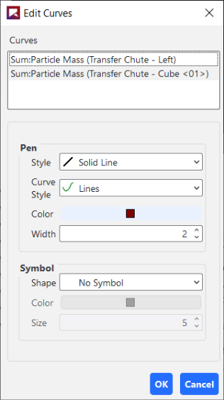
Table 1: Edit Curves dialog options
Setting | Description | Range |
|---|---|---|
Curves | Enables you to select which data set(s) you want to change. | Options limited by the plot or histogram selected |
Pen | ||
Style | For plots only (not histograms), this enables you to set what kind of line style you want represented for the selected data set. Tip: If you want the data set represented on the plot by symbols instead of lines, select No Line and then choose what you want under Symbol. | No Line; Solid Line; Dash Line; Dot Line; Dash Dot Line; Dash Dot Dot Line |
Curve Style | For plots only (not histograms), when you select a Style other than No Line, this enables you to set how the data set is represented in the plot. What you set here will be drawn in the Style indicated. | Lines; Sticks; Steps |
Color | For histograms, and also for plots with a Style other than No Line, this enables you to change the color of the bar or plot line for the selected data set. | Options limited by the Select Color dialog |
Width | For plots only (not histograms), when you select a Style other than No Line, this enables you to change the width of the plot line for the selected data set. | Whole numbers greater than or equal to one |
Symbol | ||
Shape | For plots only (not histograms), this enables you to add to the plot a symbol marking the curve's data point. For Time Plots and Multi Time Plots, a symbol will appear for each recorded output time. (For example, every 0.05s.) Tip: If you want the data set represented on the plot by lines instead of symbols, select No Symbol and then choose what you want under Pen. | Ellipse; Rectangle; Diamond; Triangle; Down Triangle; No Symbol |
Color | For plots only (not histograms), when you select a Shape other than No Symbol, this enables you to change the color of the symbol used to mark the data points of the curve. | Options limited by the Select Color dialog |
Size | For plots only (not histograms), when you select a Shape other than No Symbol, this enables you to change the size of the symbol used to mark the data points of the curve. | Whole, positive values |
TO CHANGE THE APPEARANCE OF A PLOT LINE, BAR, OR POINT:
Directly within the plot or histogram window, double-click the line, bar, or point that you want to change. The Edit Curves dialog appears.
From the Curves box, select the data set(s) you want to modify.
Under Pen and Symbol, select the options you want.
Click OK. The changes you made are reflected in the plot or histogram window.
See Also:
RECOGNIZE SHARED PARAMETERS WITH ASTERISKS (*)
Occasionally, Module parameters in Rocky will be shared by parameters of other Modules. This means that a value entered in one location in the Rocky UI will be automatically duplicated in the other location.
To help you understand when this is happening, Rocky will place an asterisk (*) after the parameter name that is being shared. If you then hover your mouse cursor over the field for that asterisked parameter (Figure 1), the tooltip that appears will tell you what other Modules are sharing that same parameter.
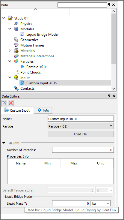
In the example shown in Figure 1, the asterisk following the name of the Liquid Mass* parameter indicates that there are one or more identical Liquid Mass parameter(s) being defined elsewhere in the Rocky UI. When you view the tooltip for this parameter's field, you learn that this parameter is shared by two separate Modules, this one included.
If you change the value for this shared parameter, it will automatically be updated in the other location(s).
Note: In this version of Rocky, the Liquid Bridge Model Module is provided as an external module. Refer to the Install an External Module topic for details.
See Also:
USE COLORED DIRECTIONAL HANDLES
When viewed in a 3D View window, you can change the shape and location of some User Process, Volume Fill, and Region of Interest shapes by using the colored directional handles, as shown in Figures 1 and 2 below.
For shapes like Cubes and Cylinders (Figure 1), the colors of the handles are defined in Table 1.
Table 1: Handle color definitions for shapes
Handle (Dot) Color | Corresponds To |
|---|---|
Red | The local X axis. |
Green | The local Y axis. |
Blue | The local Z axis. |
White | The center of the shape. Note: For Volume Fill shapes, the blue dot in the center is the Seed location but this can only be moved by defining the Seed Coordinates. (See also Create a New Volume Fill Input for Particles.) |
For planes (Figure 2), the directional handles are colored according to the Font Color specified for the 3D View (see also About Using the Window Editors panel to Change the Selected 3D View). The shapes of these colored handles are defined in Table 2.
Table 2: Handle shape definitions for planes
Handle Shape | Corresponds To |
|---|---|
Dot | The location of the plane's origin. |
Arrow | The direction of the plane's normal. |
Within the 3D View window, you can click and drag these handles to the new location you want.
Tip: To move the whole shape without deforming it, do one of the following:
Move only the center handle.
Hold either the Shift or Ctrl key while you click and drag any of the outer handles with your mouse.
Or, for more precise control, you can enter exact values in the Data Editors panel.
See Also:
KEYBOARD ACCESSIBILITY AND SHORTCUTS
While Rocky was not designed for full software accessibility, it does offer some limited features for keyboard control. For example:
TAB key: Press to move from option to option within a Rocky dialog or panel.
SPACEBAR: Press to select or clear a check box, or to select buttons in panels.
UP/DOWN ARROW keys: Press to select list items within a Rocky dialog, Panel, or menu.
LEFT/RIGHT ARROW keys: Press to view different menus or to move horizontally in Rocky dialogs.
ESC key: Press to close a dialog.
ENTER: Press to select a button within Rocky dialogs.
TO VIEW THE FULL KEYBOARD SHORTCUT LIST:
From the Options menu, click Preferences.
From the Preferences dialog, under Properties, click Shortcuts.
See Also:
FILE TYPES AND FOLDERS IN ROCKY FILE
There are several unique file types and folders used in Rocky, and several common ones. Use the tables below to identify when and why certain file types and/or folder locations are used.
Note: Only the simulation project file is saved to the directory location you choose. All other files created by Rocky (marked as "System" below) are saved to a project subfolder created automatically within the same directory as your project file. System files are critical for Rocky functioning and should not be edited, moved, or deleted.
Files you choose to export out of Rocky, including animation, image, and data files, are saved to the locations you specify. See the below tables for more detail.
Table 1: File Types Used in Rocky
Type | Description | Extension |
|---|---|---|
Rocky Simulation Files | ||
Simulation project file (Rocky v4 or later) | Contains all parameters set and analyses completed for a particular simulation created in Rocky 4 or later, and is linked to the simulation output files (.rhs, .rhc, and .rhm) that are created during processing.
| .rocky |
Simulation project file (Rocky v3 only) | Contains all parameters set and analyses completed for a particular simulation created in Rocky 3, and is linked to the simulation output files (.rhs) that are created during processing. Tip: Use the extension of the simulation project file to help you determine in which version of Rocky the project was created. Projects created in older versions of Rocky will have different features than those created in Rocky v4 or later versions. | .rocky30 |
(System) Simulation output file for particles and boundaries | The particle- and boundary-related results of the simulation that are created during processing. One output file is saved per simulation output frequency; many output files make up a whole simulation.
| .rhs |
(System) Simulation output file for contacts | The contact-related results of the simulation that are created during processing. This data is required to calculate particle and boundary movement and is by default saved for each output time to help make Resuming a Stopped Simulation faster. (See also Resume Processing a Stopped Simulation.) Tip: To reduce the size of your project files, clear the Collect Contacts Data ** checkbox. (From the **Data panel, click Contacts and then from the Data Editors ** select the **Contacts tab.) (See also About Contacts.) | .rhc |
(System) Simulation output file for motions | The motion-related results of the simulation that are created during processing. One output file is saved per simulation output frequency; many output files make up a whole simulation.
| .rhm |
(System) Solver file | Used for storing information related only to the setup and calculated results of the simulation. Does not include post-processing information, such as views, graphs, or animations. | .rocky20 |
(System) Solver output files | System files containing runtime simulation information meant to be processed by the application. (See also About the Simulation Log File.) | .rocky20.log .rocky20.out .rocky20.prg |
Rocky lock file | System file used to prevent another instance of the currently active project from being modified elsewhere. This file is created automatically by Rocky every time you open a project and remains on your system until you close the project, essentially locking the project file from being changed by anyone but you as long as you have the project open. This feature is especially useful in shared computing and server environments where multiple users may be contributing to the same Rocky projects but using different computing resources. It is for this reason that modifying, moving, or deleting the lock file is not recommended unless you are certain no other copies of the project are being worked on. (See also Rocky says my project file is "locked".) | .lock |
(System) Current output file | This is where Rocky saves the initial and final output time value, which is used to determine the current output time. | _H.txt |
Rocky script file | File used to contain script information, the latter of which includes recorded steps of a repeatable UI task. (See Creating and Using Your Scripts for more information.) | .py |
Rocky archive file | File used to contain all simulation project and supporting folders necessary for sharing the simulation project and results with others, such as Rocky support. (See also Archive a Simulation Project.) | .rocky_archive |
Rocky project context file | File used to contain the setup criteria for the 3D View windows, Workspaces, and User Processes used in the project. (See also Reuse 3D View Window, Workspace, and User Process Setups in Other Projects. | .rocky_template |
Files Exported Out of Rocky | ||
Simulation statistics file | File created by exporting curves from a plot or histogram, thereby enabling the data to be viewed and/or edited in an external spreadsheet program, such as Microsoft Excel. | .csv |
Animation file | File created by exporting an animation, thereby enabling the simulation to be viewed outside of Rocky. (See About Creating and Saving an Animation for more information.) | .avi |
Image files | Used for saving or exporting a snapshot of what is currently being displayed in a window on the Workspace, or for importing into Rocky as a logo to be shown in the 3D View. | .png .jpg .bmp .pnp |
Files Imported Into Rocky | ||
3D CAD model files | Used for importing geometries into Rocky.
Note: Unlike in previous versions, none of these file types retain the component colors assigned in the CAD model upon import into Rocky. | .xgl .stl .dxf .msh |
Fluent Case file | Used for importing geometries from an Ansys Fluent case file into Rocky. Geometry component names will be retained in this scenario. Also used to specify the Ansys Fluent simulation setup for 2-Way Fluent Coupling analyses. Contains the grid, boundary conditions, solution parameters and other data related to a fluid flow simulation problem. | .cas |
Fluent Case file (compressed) | Compressed version of a Fluent Case file (CAS). Used both for importing geometries from an Ansys Fluent case file into Rocky, and also to specify the Ansys Fluent simulation setup for 2-Way Fluent Coupling analyses. | .cas.gz |
Fluent Case file (HDF5) | Hierarchical Data Format (HDF) version of a Fluent Case file (CAS). In this version of Rocky, CAS.H5 files can be used both for importing geometries, and to specify the Ansys Fluent simulation setup for 2-Way Fluent Coupling analyses. | .cas.h5 |
Fluent Mesh file | Used for importing geometries from Ansys Fluent into Rocky. Geometry component names will not be retained when importing a MSH file into Rocky. | .msh |
Ansys Motion Functional Mock-Up Unit file | Bundled file containing all motion setup information required for a 2-Way Coupled simulation with Ansys Motion, including geometries. As such, can be used for geometry import into Rocky. Currently supports only rigid bodies (no flexible bodies) without beam elements. (For more information about beam elements, refer to your Ansys Motion documentation.) Geometry component names will be retained with this type of file import. Important: Only FMU files generated by Ansys Motion will support geometry import into Rocky. | .fmu |
Ansys Motion Geometry file | Used for importing geometries from an Ansys Motion file into Rocky. Currently supports only rigid bodies (no flexible bodies) without edge elements. Geometry component names will be retained with this type of file import. | .dfg |
Fluent to Rocky file | File generated by the Fluent plug-in installed by Rocky. Used for importing fluid flow data out of Ansys Fluent and into Rocky. Depending upon the export type chosen, produces either a static or transient fluid flow model within the simulation. (See About Using the 1-Way Fluent Method for more information.) | .f2r |
Fluent Data file | File containing Fluent initialization settings and the values of the specified flow field that can be used during a 1-Way Fluent or 2-Way Fluent coupling simulation. (See also About Using the 1-Way Fluent Method and About Using the 2-Way Fluent Method.) | .dat |
Fluent Mesh Data file | File containing CFD mesh location data that can be used in a 1-Way Fluent coupling simulation. (See also About Using the 2-Way Fluent Method.) | mesh.dat |
Fluent Data file (Compressed) | Compressed version of a Fluent Data file (DAT), which is an optional file containing Fluent initialization settings that are used during a 2-Way Fluent coupling simulation. (See also About Using the 2-Way Fluent Method.) | .dat.gz |
Fluent Data file (HDF5) | Hierarchical Data Format (HDF) version of a Fluent data file (DAT), which is an optional file containing Fluent initialization settings that are used during a 2-Way Fluent coupling simulation. (See also About Using the 2-Way Fluent Method.) | .dat.h5 |
Custom Fiber definition file | Text or spreadsheet file used to define the Segment details that make up a Custom Fiber shape. (See also About Defining and Importing Custom Particle Shapes.) | .txt .csv .xls .xlsx .xlsm .xlsb .odf |
Custom Input definition file | Spreadsheet file used to define the particle positioning details that make up a Custom Input. (See also About Adding and Editing Particle Inputs.) | .csv .xls .xlsx .xlsm .xlsb .odf |
Point Cloud definition file | Text file used to define the details that make up a Point Cloud. (See also About Point Clouds.) | .txt |
Table 2: Common Folder Locations Used in Rocky
Folder | Typical Windows Location | Typical Linux Location | Description |
|---|---|---|---|
Rocky Settings |
|
| Folder where Rocky stores settings that persist from project to project. These include license settings, a list a list of recently opened projects, and a separate "Settings" folder that contains your display and interaction preferences. (See below.) |
Rocky Preferences |
|
| Folder where Rocky saves user preferences for various display and interaction settings. These settings can be established by users in the Preferences dialog (see also About Setting Global Preferences), or in several other Rocky locations by clicking a Save Current Configuration in Settings button. Both the values displayed on the Preferences dialog and the ones displayed on the UI element after the Restore Configuration from Settings button is clicked reflects the values saved to this folder. |
User Manual Cache |
|
| Contains the cache for the user manual. |
Shared PrePost Scripts |
|
| Folder where Rocky saves scripts you recorded on the Scripts shared across projects tab of the PrePost Script panel. Also where you save PY script files that have been created outside of Rocky using the API:PrePost functionality. (See also Creating and Using Your Scripts.) |
Project-Only PrePost Scripts |
|
| Folder where Rocky saves scripts you recorded on the Project scripts tab of the PrePost Script panel. Also where you save PY script files that have been created outside of Rocky using the API:PrePost functionality. (See also Creating and Using Your Scripts.) |
External Modules |
|
| Folder where you save the compiled external Module that you either create yourself or download from the Customer Portal. |
Tip: Performing a clean install of Rocky may involve renaming and/or archiving these folders after uninstalling Rocky and prior to reinstalling it. (See also I reinstalled Rocky but I am still seeing errors.)
See Also:
The simulation log is one of the solver output files that Rocky provides while processing a project. (See also File Types and Folders in Rocky). It contains simple information, such as hardware details, to more complex data about the simulation, such as particles, triangles, and contacts information; memory consumption and free memory; and other solver process information.
To access the simulation log file for a specific project, follow the steps below:
Navigate to the folder containing the project for which you want to see simulation details.
Open the project_name.rocky.files folder.
Open the simulation folder.
The simulation log file is located inside the simulation folder and is named rocky_simulation.rocky20.log (as shown in Figure 1). It is a Text Document, so you can open it with any text editor.
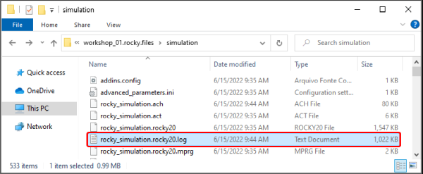
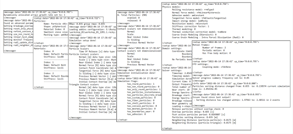
Inside the file, information is arranged similarly to the figures shown in this section. Some key areas are enumerated and explained below.
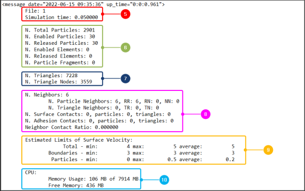
In Figure 2 (shown below), you can see the following:
Product release and version used to process the Rocky project. (See also About This Version of Rocky.)
License file information
Hardware details
Used licenses. (See also Verify Your Rocky License Status.)

Next, you will see everything that is related to the project setup including the physical models enabled, particle groups defined, materials, boundary limits, solver options, coupling mode, motion frames, and more (Figure 3).
After that, the file shows a structure (Figures 4 and 5) that repeats for each output time and contains the following details:
File number (that refers to the output time) and simulation time
Particle and fragment counts. (See also About Particle Breakage.)
Triangle counts
Contact counts and ratios. (See also About Contacts.)
Limits of surface velocity
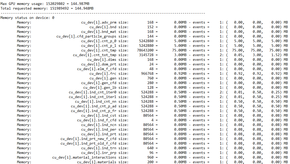
Memory (consumption and availability). (See also About the Cache Panel.)
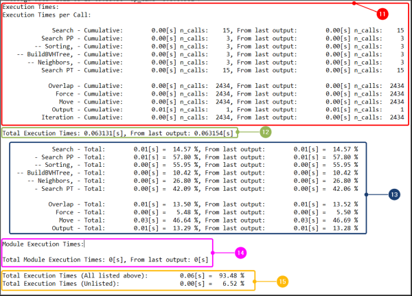
Average time per call and number of calls for each process. Note: Depending on the case, the processes will be different.
Execution times: both the total and since the last output
Total execution time, which is the average time per call multiplied by the number of calls
Execution times for the module: both the total and since the last output
Total execution times, which are the total measured and segregated times by the solver in the last output plus the fraction of time not measured by the solver
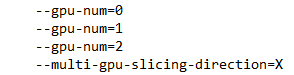
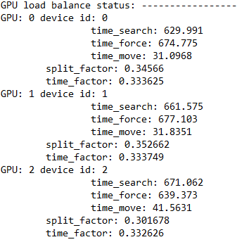
Finally, we have some additional information for simulations with GPU usage. Figures 6-8 show an example of a simulation log file for a project processed with 3 GPUs. The data shown includes the following:
GPUs IDs
GPU load balance with the time spent in each process and the split factor.
Tip: The slipt factor indicates the memory consumption of the GPU in relation to the total memory consumption (from all GPUs). In this example, as we have 3 GPUs, the ideal is to have a split factor close to 0.333.
Memory consumed in each device
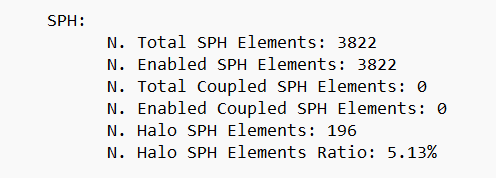
N. Halo SPH Elements/Halo Particles: In multi-GPU runs, halo particles/elements are those that are located in the overlapping devices domain regions and therefore are present simultaneously in two GPU devices. For the halo particles/elements, both devices compute the collision forces, but only one of the devices accumulates these data in order to perform velocity and displacement calculations.
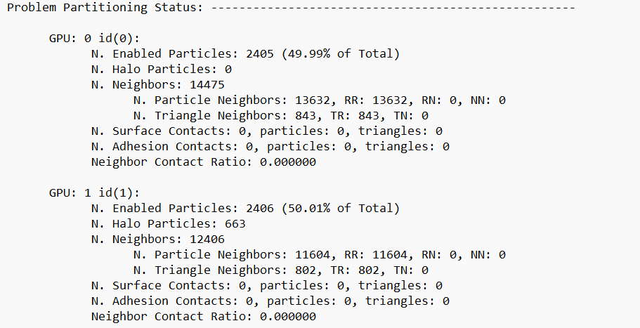
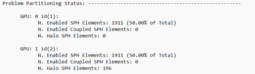
Problem Partitioning Status: This parameter represents the number of SPH Elements or particles coupled in the simulation.
N. Enabled Coupled SPH Elements: It is the number of SPH elements figured inside the particles for the purpose of interacting with external SPH elements in an SPH-DEM interaction simulation. This parameter will only be computed in simulations with SPH and DEM, otherwise it will appear as zero.
Note: If you processed your simulation without GPU usage, your simulation log file will not show this data. You can see how many GPUs were used by looking at the section marked "3" in Figure 1. (In that simulation example, "Use GPU: 0" means that the project was processed without GPU usage.)