


The properties presented on the Properties and Curves tabs represent the many different statistics that Rocky records at each timestep for each individual element in a structure (e.g., particle, air flow node, geometry triangle) as your simulation processes. The large amount of data that Rocky collects is then distilled into default properties that are accessible from either the Properties or Curves tab for the entity of interest.
Once a property is selected, you can quickly display individual statistics, visualize the data set in a 3D View, graph them in a plot or histogram, or export them in tabular format. You may also customize the default properties Rocky provides to create your own unique data sets, including limiting properties by a specific time range by using Time Statistics.
Note: The process for customizing default properties for Eulerian Statistics User Processes is slightly different from other entities. (See also About Customizing Eulerian Statistics Properties.)
If you need to distill a data set from a property into one final value, or analyze the components that make up your data set, you can do so from the Output tab of the Expressions/Variables panel (see also About Defining Output Variables).
To help you choose the correct property, Rocky separates them into the following two categories:
Properties contain data sets that include recorded values for each individual element in a structure at each individual timestep during the simulation. This has the potential of producing many unique values per timestep.
Curves contain data sets that apply to the entire entity as a whole, producing only one value for each property.
Note: For any particles that you have defined as Multiple Element (meshed), what you have set for Meshed Particles Upscaling affects whether and how some post-processing properties and curves are displayed (see also About Meshed Particles Upscaling).
What would you like to do?
Learn more About Properties
Learn more About Curves
Learn more About Customizing Properties or Curves
Learn more About Adding and Editing Time Statistics Properties
Learn more About Meshed Particles Upscaling
Change or Remove an Existing Custom Property on the Properties or Curves Tab
Add a Particle Property to a Eulerian Statistics User Process
See Also:
Properties are data sets that include recorded values for each individual element in a structure (e.g., particle, geometry triangle, or air flow node) at each individual output time during the simulation.
Because they have the potential to produce many unique values for each output time, Properties must first be limited by some factor (e.g., showing the data for only one output at a time, showing only the minimum or average value for all output times, and so on) before displaying it in the Rocky UI.
The ways in which you can limit and display your Properties are described in Table 1.
Table 1: Methods for Limiting What a Property will Display
Limit By | Method | See Also |
|---|---|---|
Operations | ||
By operations only | Create a Time Plot from the property and then choose to limit the values by one of the operations provided, which include Min, Max, Sum, Sum Squared, Average, Variance, and Std. Deviation. | |
By both output time and operations | From the property, choose to Compute Statistics for a single output time and then use the UI to display the individual values you want. The values you can display include the same operations used to limit a Time Plot (Min, Max, and so on) but also include Name, Unit, Type, and Location. | |
Output Time Only | ||
By creating a 3D View window | Create a 3D View from the function and then use the Time toolbar to walk through the data collected for each individual output time (see also About the Time Toolbar). | |
By creating a Particles Details window | For Intra-Particle Collision Statistics properties only (see also About Intra-Particle Collision Statistics), create a Particles Details window from the function and then use the Time toolbar to walk through the data collected for each individual output time (see also About the Time Toolbar). | |
By creating a Histogram | Create a Histogram from the property and then use the Time toolbar to walk through the data collected for each individual output time (see also About the Time Toolbar). |
Rocky calculates Properties for individual geometry components, including conveyors and imported geometries; Particles, Contacts, 1-Way LBM, 1-Way Fluent, 2-Way Fluent, Eulerian Statistics, various kinds of Collision Statistics, and individual User Processes based upon these entities.
Note: When displaying Properties for a User Process, the properties displayed will be those belonging to the linked entity upon which the User Process was based (see also See Input/Output Relationships in the Data Panel When Component Names are Bold).
If these default properties do not meet your needs, you may also create custom Properties (see also About Customizing Properties or Curves), including Time Statistics Properties, which limits properties by a time range (see also About Adding and Editing Time Statistics Properties).s
A list of available properties appears for each applicable component after processing via the component's Properties tab. Next to each property name row are various columns representing specific categories of operations and other data (Figure 5.1: Example Properties tab showing all available data columns).
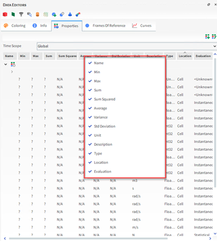
Besides separate columns for all standard operators—which include values for Min, Max, Sum, Sum Squared, Average, Variance, and Std. Deviation—you can also view the property's Units, Type, Location, and Evaluation.
By right-clicking a property row and then selecting Compute statistics, you can get values for that property at that particular output (see also About Viewing an Individual Statistic).
See the images and tables below to learn about the various Properties available by default in Rocky.
Table 2: Properties available by default for all entities
Property Name | Description |
|---|---|
Time Scope | Sets how the resulting statistics are displayed in the various factor columns. Specifically:
|
There are two kinds of Properties for individual Geometry components:
Standard properties, which are calculated by default for every conveyor or imported Geometry (Figure 5.3: Standard Properties options on the Data Editors panel for Geometry components - see also Add and Edit Geometry Components).
Collision statistics properties, which are collected only when the Boundary Collision Statistics collection feature is enabled (Figure 5.4: Collisions Statistics Properties on the Data Editors panel for Geometry components - see also About Collision Statistics for Boundaries).

Table 3: Properties available by default for Geometries (Feed Conveyors, Receiving Conveyors, and Imported) (see also I cannot find some Geometry Properties or Curves in this version of Rocky).
Property Name | Description |
|---|---|
Standard Properties | |
Area : Cell | The surface area of each individual triangle that makes up the selected geometry. For chutes with wear modification parameters, this is useful for estimating how much surface area might be worn away due particle impact (see Enable and View Surface Wear Modification on an Imported Geometry). |
Area : Nodal | The area of a region around each individual geometry node. This area is equal to the sum of one third of the area of all triangles that share a given node. This is useful for analyzing the amount of wear on a surface due to shear work. |
Coordinate : Nodal : X | The coordinate location along the X axis for each individual geometry node. This is useful for analyzing the amount of shear wear in the X direction. |
Coordinate : Nodal : Y | The coordinate location along the Y axis for each individual geometry node. This is useful for analyzing the amount of shear wear in the Y direction. |
Coordinate : Nodal : Z | The coordinate location along the Z axis for each individual geometry node. This is useful for analyzing the amount of shear wear in the Z direction. |
Displacement : X | For imported geometries with surface wear modification enabled (see also Enable and View Surface Wear Modification on an Imported Geometry), this is the distance that each triangle's vertex was displaced by wear in the X direction. |
Displacement : Y | For imported geometries with surface wear modification enabled (see also Enable and View Surface Wear Modification on an Imported Geometry), this is the distance that each triangle's vertex was displaced by wear in the Y direction. |
Displacement : Z | For imported geometries with surface wear modification enabled (see also Enable and View Surface Wear Modification on an Imported Geometry), this is the distance that each triangle's vertex was displaced by wear in the Z direction. |
Temperature | When Thermal Model is enabled (see also Enable Thermal Modeling Calculations), this is the thermodynamic temperature of each individual triangle that makes up the selected geometry. |
Boundary Collision Statistics Properties | |
Duration : Kurtosis | When the Duration option is enabled on the Boundary Collision Statistics module (see also About Collision Statistics for Boundaries), this provides the Kurtosis value of the duration of the collisions recorded in different regions of the geometry during an interval between two consecutive output time. The kurtosis is a measure of how tall and sharp the central peak of a statistical distribution is. See also the "Collision statistics" section of the DEM Technical Manual (from the Rocky Help menu, point to Manuals, and then click DEM Technical Manual). |
Duration : Mean | When the Duration option is enabled on the Boundary Collision Statistics module (see also About Collision Statistics for Boundaries), this provides the mean value of the duration of the collisions recorded in different regions of the geometry, during an interval between two consecutive output times. See also the "Collision statistics" section of the DEM Technical Manual (from the Rocky Help menu, point to Manuals, and then click DEM Technical Manual). |
Duration : Skewness | When the Duration option is enabled on the Boundary Collision Statistics module (see also About Collision Statistics for Boundaries), this provides the skewness value of the duration of the collisions recorded in different regions of the geometry, during an interval between two consecutive output times. The skewness is a measure of the asymmetry of a statistical distribution about its mean. See also the "Collision statistics" section of the DEM Technical Manual (from the Rocky Help menu, point to Manuals, and then click DEM Technical Manual). |
Duration : Std. Dev. | When the Duration option is enabled on the Boundary Collision Statistics module (see also About Collision Statistics for Boundaries), this provides the standard deviation value of the duration of the collisions recorded in different regions of the geometry, during an interval between two consecutive output times. See also the "Collision statistics" section of the DEM Technical Manual (from the Rocky Help menu, point to Manuals, and then click DEM Technical Manual). |
Force : Nodal : X | When the Forces for FEM Analysis option is enabled on the Boundary Collision Statistics module (see also About Collision Statistics for Boundaries), this provides the average force in the X direction for each individual geometry node. See also the "Collision statistics" section of the DEM Technical Manual (from the Rocky Help menu, point to Manuals, and then click DEM Technical Manual). |
Force : Nodal : Y | When the Forces for FEM Analysis option is enabled on the Boundary Collision Statistics module (see also About Collision Statistics for Boundaries), this provides the average force in the Y direction for each individual geometry node. See also the "Collision statistics" section of the DEM Technical Manual (from the Rocky Help menu, point to Manuals, and then click DEM Technical Manual). |
Force : Nodal : Z | When the Forces for FEM Analysis option is enabled on the Boundary Collision Statistics module (see also About Collision Statistics for Boundaries), this provides the average force in the Z direction for each individual geometry node. See also the "Collision statistics" section of the DEM Technical Manual (from the Rocky Help menu, point to Manuals, and then click DEM Technical Manual). |
Frequency | When the Frequency option is enabled on the Boundary Collision Statistics module (see also About Collision Statistics for Boundaries), this provides the average collision frequency recorded in different regions of the geometry, during an interval between two consecutive output times. See also the "Collision statistics" section of the DEM Technical Manual (from the Rocky Help menu, point to Manuals, and then click DEM Technical Manual). |
Intensity | When the Intensities option is enabled on the Boundary Collision Statistics module (see also About Collision Statistics for Boundaries), this, for each triangle on a boundary, provides the average power needed to move it with the prescribed velocity, divided by the triangle's area. See also the "Collision statistics" section of the DEM Technical Manual (from the Rocky Help menu, point to Manuals, and then click DEM Technical Manual). |
Intensity : Dissipation | When the Intensities option is enabled on the Boundary Collision Statistics module (see also About Collision Statistics for Boundaries), this provides the average power dissipated by the contact forces, divided by the triangle's area, measured by each individual geometry triangle. See also the "Collision statistics" section of the DEM Technical Manual (from the Rocky Help menu, point to Manuals, and then click DEM Technical Manual). |
Intensity : Impact | When the Intensities option is enabled on the Boundary Collision Statistics module (see also About Collision Statistics for Boundaries), this provides the average impact power measured by each individual triangle and divided by the triangle's area. This is useful for determining impact wear on geometry surfaces. See also the "Collision statistics" section of the DEM Technical Manual (from the Rocky Help menu, point to Manuals, and then click DEM Technical Manual). |
Intensity : Shear | When the Intensities option is enabled on the Boundary Collision Statistics module (see also About Collision Statistics for Boundaries), this provides the average shear power measured by each individual triangle. This is useful for determining shear wear on geometry surfaces. See also the "Collision statistics" section of the DEM Technical Manual (from the Rocky Help menu, point to Manuals, and then click DEM Technical Manual) |
Sliding Distance : Kurtosis | When the Sliding Distance option is enabled on the Boundary Collision Statistics module (see also About Collision Statistics for Boundaries), this provides the Kurtosis value of the sliding distance, which is the distance that a particle moves during a collision, parallel to the boundary triangle plane where the collision occurs. This is useful for determining boundary wear caused by shear. See also the "Collision statistics" section of the DEM Technical Manual (from the Rocky Help menu, point to Manuals, and then click DEM Technical Manual). |
Sliding Distance : Mean | When the Sliding Distance option is enabled on the Boundary Collision Statistics module (see also About Collision Statistics for Boundaries), this provides the mean value of the sliding distance, which is the distance that a particle moves during a collision, parallel to the boundary triangle plane where the collision occurs. This is useful for determining boundary wear caused by shear. See also the "Collision statistics" section of the DEM Technical Manual (from the Rocky Help menu, point to Manuals, and then click DEM Technical Manual). |
Sliding Distance : Skewness | When the Sliding Distance option is enabled on the Boundary Collision Statistics module (see also About Collision Statistics for Boundaries), this provides the Skewness value of the sliding distance, which is the distance that a particle moves during a collision, parallel to the boundary triangle plane where the collision occurs. This is useful for determining boundary wear caused by shear. See also the "Collision statistics" section of the DEM Technical Manual (from the Rocky Help menu, point to Manuals, and then click DEM Technical Manual). |
Sliding Distance : Std. Dev. | When the Sliding Distance option is enabled on the Boundary Collision Statistics module (see also About Collision Statistics for Boundaries), this provides the standard deviation value of the sliding distance, which is the distance that a particle moves during a collision, parallel to the boundary triangle plane where the collision occurs. This is useful for determining boundary wear caused by shear. See also the "Collision statistics" section of the DEM Technical Manual (from the Rocky Help menu, point to Manuals, and then click DEM Technical Manual). |
Stress : Adhesive | When the Stresses option is enabled on the Boundary Collision Statistics module (see also About Collision Statistics for Boundaries), an Adhesive Force model (other than None) is enabled (see also About Physics Parameters), and an Adhesive Force Fraction for a boundary-boundary and/or boundary-particle Materials Interaction pair has a value set higher than zero (see also About Modifying Materials Interactions and Adhesion Values), this provides the average adhesive stress in the normal direction, as measured by each individual geometry triangle. See also the "Collision statistics" section of the DEM Technical Manual (from the Rocky Help menu, point to Manuals, and then click DEM Technical Manual). |
Stress : Normal | When the Stresses option is enabled on the Boundary Collision Statistics module (see also About Collision Statistics for Boundaries), this provides the average normal stress measured by each individual geometry triangle. See also the "Collision statistics" section of the DEM Technical Manual (from the Rocky Help menu, point to Manuals, and then click DEM Technical Manual). |
Stress : Tangential | When the Stresses option is enabled on the Boundary Collision Statistics module (see also About Collision Statistics for Boundaries), this provides the average tangential stress measured by each individual geometry triangle. See also the "Collision statistics" section of the DEM Technical Manual (from the Rocky Help menu, point to Manuals, and then click DEM Technical Manual). |
Velocity : Impact : Normal : Kurtosis | When the Normal Impact Velocity option is enabled on the Boundary Collision Statistics module (see also About Collision Statistics for Boundaries), this provides the kurtosis value of the impact relative velocity in the normal direction resulting from the collisions recorded in different regions of the geometry, during an interval between two consecutive output times. The kurtosis is a measure of how tall and sharp the central peak of a statistical distribution is. See also the "Collision statistics" section of the DEM Technical Manual (from the Rocky Help menu, point to Manuals, and then click DEM Technical Manual). |
Velocity : Impact : Normal : Mean | When the Normal Impact Velocity option is enabled on the Boundary Collision Statistics module (see also About Collision Statistics for Boundaries), this provides the mean value of the impact relative velocity in the normal direction resulting from the collisions recorded in different regions of the geometry, during an interval between two consecutive output times. See also the "Collision statistics" section of the DEM Technical Manual (from the Rocky Help menu, point to Manuals, and then click DEM Technical Manual). |
Velocity : Impact : Normal : Skewness | When the Normal Impact Velocity option is enabled on the Boundary Collision Statistics module (see also About Collision Statistics for Boundaries), this provides the skewness value of the impact relative velocity in the normal direction resulting from the collisions recorded in different regions of the geometry, during an interval between two consecutive output times. The skewness is a measure of the asymmetry of a statistical distribution about its mean. See also the "Collision statistics" section of the DEM Technical Manual (from the Rocky Help menu, point to Manuals, and then click DEM Technical Manual). |
Velocity : Impact : Normal : Std. Dev. | When the Normal Impact Velocity option is enabled on the Boundary Collision Statistics module (see also About Collision Statistics for Boundaries), this provides the standard deviation value of the impact relative velocity in the normal direction resulting from the collisions recorded in different regions of the geometry, during an interval between two consecutive output times. See also the "Collision statistics" section of the DEM Technical Manual (from the Rocky Help menu, point to Manuals, and then click DEM Technical Manual). |
Velocity : Impact : Tangential : Kurtosis | When the Tangential Impact Velocity option is enabled on the Boundary Collision Statistics module (see also About Collision Statistics for Boundaries), this provides the Kurtosis value of the impact relative velocity in the tangential direction resulting from the collisions recorded in different regions of the geometry, during an interval between two consecutive output times. The kurtosis is a measure of how tall and sharp the central peak of a statistical distribution is. See also the "Collision statistics" section of the DEM Technical Manual (from the Rocky Help menu, point to Manuals, and then click DEM Technical Manual). |
Velocity : Impact : Tangential : Mean | When the Tangential Impact Velocity option is enabled on the Boundary Collision Statistics module (see also About Collision Statistics for Boundaries), this provides the mean value of the impact relative velocity in the tangential direction resulting from the collisions recorded in different regions of the geometry, during an interval between two consecutive output times. See also the "Collision statistics" section of the DEM Technical Manual (from the Rocky Help menu, point to Manuals, and then click DEM Technical Manual). |
Velocity : Impact : Tangential : Skewness | When the Tangential Impact Velocity option is enabled on the Boundary Collision Statistics module (see also About Collision Statistics for Boundaries), this provides the skewness value of the impact relative velocity in the tangential direction resulting from the collisions recorded in different regions of the geometry, during an interval between two consecutive output times. The skewness is a measure of the asymmetry of a statistical distribution about its mean. See also the "Collision statistics" section of the DEM Technical Manual (from the Rocky Help menu, point to Manuals, and then click DEM Technical Manual). |
Velocity : Impact : Tangential : Std. Dev. | When the Tangential Impact Velocity option is enabled on the Boundary Collision Statistics module (see also About Collision Statistics for Boundaries), this provides the standard deviation value of the impact relative velocity in the tangential direction resulting from the collisions recorded in different regions of the geometry, during an interval between two consecutive output times. See also the "Collision statistics" section of the DEM Technical Manual (from the Rocky Help menu, point to Manuals, and then click DEM Technical Manual). |
There are several kinds of Properties that can affect all Particles in the simulation. These include:
Standard properties, which are calculated by default and are applicable to all particle sets in the simulation (Figure 5.5: Particles, Standard Property options in the Data Editors panel. See also About Adding and Editing Particle Sets).
Inter-particle Collision statistics properties, which are collected for all Particles only when the Inter-particle Collision Statistics collection feature is enabled (Figure 5.6: Particles, Property options in the Data Editors panel when Inter-particle Collision Statistics are collected. See also About Inter-particle Collision Statistics). Note: Some Inter-particle Collision Statistics properties will not be provided for meshed particles with Meshed Particles Upscaling enabled (see also About Meshed Particles Upscaling).
Particle Instantaneous Energies properties, which are collected for all Particles only when the Particle Instantaneous Energies collection feature is enabled (Figure 5.7: Particles, Property options in the Data Editors panel when Particle Instantaneous Energies are collected. See also About Particle Instantaneous Energies).
Coarse Grain Modeling (CGM) properties, which appear for all Particles only when the CGM model is enabled (see also About Physics Parameters).
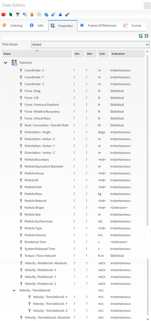
CFD Coupling Particle Statistics properties, which are collected for all Particles only when the CFD Coupling Particle Statistics collection feature is enabled (Figure 5.8: Particles, Property options in the Data Editors panel when CFD Coupling Particle Statistics are collected. See also About Fluid-Related Statistics for Particles).
Figure 5.6: Particles, Property options in the Data Editors panel when Inter-particle Collision Statistics are collected
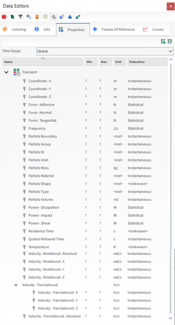
Figure 5.7: Particles, Property options in the Data Editors panel when Particle Instantaneous Energies are collected
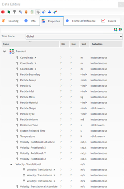
Figure 5.8: Particles, Property options in the Data Editors panel when CFD Coupling Particle Statistics are collected
Note: Due to the different ways that Rocky calculates individual particles—for example, based upon whether the particle is whole or broken into fragment (see also Enable Particle Breakage Calculations), remains single or has been meshed into multiple element (see also About Adding and Editing Particle Sets), has particle upscaling effects enabled or disabled (see also About Meshed Particles Upscaling), and so on—some Properties will not be available for particles that are meshed, or for particles that are calculated with the Meshed Particles Upscaling checkbox enabled.
Table 4: Properties available for the main Particles entity
Property Name | Description |
|---|---|
Standard Properties | |
Velocity : Rotational : Absolute |
The magnitude of the rotational velocity of each individual whole particle or fragment. This is useful for determining the angular momentum of particles, which affects particle rolling. It is defined as the norm of the particle's absolute rotational velocity vector. |
Velocity : Translational : Absolute | The magnitude of the translational velocity of each individual whole particle or fragment. This is useful for locating stalled particles in chutes, for example. It can be defined as the norm of the particle's absolute translational velocity vector. |
Flip Count | For non-flexible, shaped particle only, this is the number of times a whole particle makes a complete, 360 degree turn inside a region. It is useful for measuring coating efficiency for pills and snack foods (see also About Particles Calculations). Note: This Property is not compatible with Breakage calculations (see also Enable Particle Breakage Calculations) nor with particles composed of multiple element (flexible). |
Laguerre-Voronoi Size | When Instantaneous Breakage parameters are enabled (see also Enable Particle Breakage Calculations), this is the diameter of a sphere used to generate the fragment using the Laguerre-Voronoi tessellation. It can be defined as twice the minimum distance between the particle's center of mass and the particle's sides:
where:
Note: This property is not defined for fragments that result from Discrete Breakage events. |
Moment of Inertia | The moment of inertia of each individual whole particle or fragment. Notes:
|
Orientation : Angle | This angle together with the Orientation Vector defines the instantaneous orientation of each individual whole particle or fragment. See also the "Particle orientation" section of the DEM Technical Manual (from the Rocky Help menu, point to Manuals, and then click DEM Technical Manual). These properties illustrate how much each particle has rotated and can be useful in pharmaceutical applications where the efficiency of coating is affected by the pill's orientation in relation to the equipment. Note: Does not apply to meshed particles with particles upscaling enabled. (See also About Meshed Particles Upscaling.) |
Orientation : Vector : X | The x-axis component of a unit vector that defines the axis of rotation, which, together with the Orientation Angle, specifies the instantaneous orientation of each individual whole particle or fragment. See also the "Particle orientation" section of the DEM Technical Manual (from the Rocky Help menu, point to Manuals, and then click DEM Technical Manual). Note: Does not apply to meshed particles with particles upscaling enabled (see also About Meshed Particles Upscaling). |
Orientation : Vector : Y | The y-axis component of a unit vector that defines the axis of rotation, which, together with the Orientation Angle, specifies the instantaneous orientation of each individual whole particle or fragment. See also the "Particle orientation" section of the DEM Technical Manual (from the Rocky Help menu, point to Manuals, and then click DEM Technical Manual). Note: Does not apply to meshed particles with particles upscaling enabled (see also About Meshed Particles Upscaling). |
Orientation : Vector : Z | The z-axis component of a unit vector that defines the axis of rotation, which, together with the Orientation Angle, specifies the instantaneous orientation of each individual whole particle or fragment. See also the "Particle orientation" section of the DEM Technical Manual (from the Rocky Help menu, point to Manuals, and then click DEM Technical Manual). Note: Does not apply to meshed particles with particles upscaling enabled (see also About Meshed Particles Upscaling). |
Parent ID | For simulations with Instantaneous Breakage parameters enabled (see also Enable Particle Breakage Calculations), this index is used to identify the original whole particle or fragment from which the broken fragments were generated. Specifically:
Tip: To identify all the particle fragments that were generated within a simulation, use the Property User Process to select Parent IDs with values equal to and greater than zero (see also About the Property User Process). |
Particle Boundary | The name of the geometry source (i.e., feed conveyor or inlet) through which each individual whole particle originally entered the simulation, and which is then inherited by any fragments that are generated. Particle Boundaries are numbered from zero in (roughly) the order in which they were added. |
Particle Equivalent Diameter | The diameter of a sphere with the same volume of the whole particle or fragment.
Note: Does not apply to meshed particles with particles upscaling enabled (see also About Meshed Particles Upscaling). |
Particle Group | The name of the Particle set to which each individual whole particle originally belonged, and which is also inherited by any fragment that are generated. Particle Groups are numbered from zero in (roughly) the order in which they were added. Tip: The numbers are needed, in part, when creating a Property User Process (see also About the Property User Process). Use the Color scale to map the numbers to the Particle Group name (see also About Color Scales). |
Particle ID | The numeric identifier unique to each individual whole particle or fragment. |
|
Particle Inlet |
The name of the inlet through which each individual whole particle originally entered the simulation. |
|
Particle Mass |
The mass of each individual whole particle or fragment. |
Particle Material | The material assigned to each individual whole particle, which is then inherited by any fragments that are generated. By default, this is "Default Particles" (see also About Modifying Material Compositions). Particle Materials are numbered from zero in (roughly) the order in which they were created. |
Particle Shape | The Shape name category to which each individual whole particle in each Particle set was originally assigned, including its fragment, which inherit this value. Particle Shapes are numbered from zero in (roughly) the following order:
Note: This property replaces the now legacy Particle Type property. Tip: The numbers are needed, in part, when creating a Property User Process (see also About the Property User Process). Use the Color scale to map the numbers to the Particle Shape type (see also About Color Scales). |
Particle Size | The sieve size of each individual whole particle or fragment, which is based upon the dimensions of a square hole just big enough for the particle to pass through. This use of virtual "mesh" determines the size of the particles no matter what shape they are. Note: Does not apply to meshed particles with particles upscaling enabled (see also About Meshed Particles Upscaling). |
Particle Surface Area | The surface area of each individual whole particle or fragment. Note: Applies only to non-meshed particles (see also About Adding and Editing Particle Sets). |
Particle Type (Legacy Use Only) | Important: This property does not reflect newer particle types and is retained only for compatibility purposes. For new projects, use the Particle Shape Property instead. For projects created prior to Rocky v4.1, this is the shape type assigned to each individual whole particle, which is then inherited by any fragment that are created (see also About Adding and Editing Particle Sets). The particle type number maps to the particle shapes as follows:
|
Particle Volume | The volume of each individual whole particle or fragment. |
Coordinate : X | The coordinate location along the X-axis for each individual whole particle or fragment. |
Coordinate : Y | The coordinate location along the Y-axis for each individual whole particle or fragment. |
Coordinate : Z | The coordinate location along the Z-axis for each individual whole particle or fragment. |
Residence Time | The amount of time each individual whole particle or fragment has been within the specified
region boundaries (see also About
Particles Calculations). It can be defined as the difference between
the current time,
Particle fragments initially inherit this value from their parent upon breaking, but are then calculated separately. For example, if a fragment tumbles out of the selection and then re-enters it later, its Residence Time will increase. Note: This Property is not compatible with projects processed with earlier versions of Rocky (prior to Rocky v4) that also had breakage modeling enabled (see also Enable Particle Breakage Calculations). |
| Velocity : Rotational : X | The x-component of the rotational velocity vector of each individual whole particle or fragment. |
Velocity : Rotational : Y | The y-component of the rotational velocity vector of each individual whole particle or fragment. |
Velocity : Rotational : Z | The z-component of the rotational velocity vector of each individual whole particle or fragment. |
Stress Tensor | When the Collect Contacts Data checkbox is enabled (see also
About Contacts), this provides the
stress tensor of a particle
where:
Notes:
|
System Released Time | The instance in simulation time when each individual whole particle or fragment originally entered the simulation boundaries. |
Temperature | When Thermal Model is enabled (see also Enable Thermal Modeling), this is the thermodynamic temperature of each individual whole particle and fragment. |
Velocity : Translational : Absolute | The translational velocity vector of each individual whole particle or fragment, the magnitude of which is made up of the x, y, and z components respectively. Note: Because this is a vector, display is limited to the 3D View only. When shown in a 3D view, the particles will be colored by the magnitude of the velocity vector. |
Velocity : Translational : X | The x-component of the current translational velocity vector of each individual whole particle or fragment. |
Velocity : Translational : Y | The y-component of the current translational velocity vector of each individual whole particle or fragment. |
Velocity : Translational : Z | The z-component of the current translational velocity vector of each individual whole particle or fragment. |
Inter-Particle Collision Statistics Properties | |
Duration : Kurtosis | When the Duration option is enabled on the Inter-particle Collision Statistics module (see also About Inter-particle Collision Statistics), this provides the kurtosis value of the duration of the collisions recorded by each individual whole particle or fragment during an interval between two consecutive output time. The kurtosis is a measure of how tall and sharp the central peak of a statistical distribution is. Note: Does not apply to meshed particles with particles upscaling enabled (see also About Meshed Particles Upscaling). See also the "Collision statistics" section of the DEM Technical Manual (from the Rocky Help menu, point to Manuals, and then click DEM Technical Manual). |
Duration : Mean | When the Duration option is enabled on the Inter-particle Collision Statistics module (see also About Inter-particle Collision Statistics), this provides the mean value of the duration of the collisions recorded by each individual whole particle or fragment, during an interval between two consecutive output times. Note: Does not apply to meshed particles with particles upscaling enabled (see also About Meshed Particles Upscaling). See also the "Collision statistics" section of the DEM Technical Manual (from the Rocky Help menu, point to Manuals, and then click DEM Technical Manual). |
Duration : Skewness | When the Duration option is enabled on the Inter-particle Collision Statistics module (see also About Inter-particle Collision Statistics), this provides the skewness value of the duration of the collisions recorded by each individual whole particle or fragment, during an interval between two consecutive output times. The skewness is a measure of the asymmetry of a statistical distribution about its mean. Note: Does not apply to meshed particles with particles upscaling enabled (see also About Meshed Particles Upscaling). See also the "Collision statistics" section of the DEM Technical Manual (from the Rocky Help menu, point to Manuals, and then click DEM Technical Manual). |
Duration : Std. Dev. | When the Duration option is enabled on the Inter-particle Collision Statistics module (see also About Inter-particle Collision Statistics), this provides the standard deviation value of the duration of the collisions recorded by each individual whole particle or fragment, during an interval between two consecutive output times. Note: Does not apply to meshed particles with particles upscaling enabled (see also About Meshed Particles Upscaling). See also the "Collision statistics" section of the DEM Technical Manual (from the Rocky Help menu, point to Manuals, and then click DEM Technical Manual). |
Force : Adhesive | When the Force option is enabled on the Inter-particle Collision Statistics module (see also About Inter-particle Collision Statistics), an Adhesive Force model (other than None) is enabled (see also About Physics Parameters), and an Adhesive Force Fraction for a particle-boundary and/or particle-particle Materials Interaction pair has a value set higher than zero (see also About Modifying Materials Interactions and Adhesion Values), this this provides the sum of the adhesive forces in the normal direction as recorded by each individual whole particle or fragment. |
Force : Normal | When the Force option is enabled on the Inter-particle Collision Statistics module (see also About Inter-particle Collision Statistics), this provides the sum of the normal forces recorded by each individual whole particle or fragment. |
Force : Tangential | When the Force option is enabled on the Inter-particle Collision Statistics module (see also About Inter-particle Collision Statistics), this provides the sum of the tangential forces recorded by each individual whole particle or fragment. |
Frequency | When the Frequency option is enabled on the Inter-particle Collision Statistics module (see also About Inter-particle Collision Statistics), this provides the average collision frequency recorded by each individual whole particle or fragment, during an interval between two consecutive output times. See also the "Collision statistics" section of the DEM Technical Manual (from the Rocky Help menu, point to Manuals, and then click DEM Technical Manual). |
Power : Dissipation | When the Power option is enabled on the Inter-particle Collision Statistics module (see also About Inter-particle Collision Statistics), this provides the power dissipated in the collisions of the contact forces recorded by each individual whole particle or fragment. |
Power : Impact | When the Power option is enabled on the Inter-particle Collision Statistics module (see also About Inter-particle Collision Statistics), this provides the power transferred during the loading phase of all collisions recorded by each individual whole particle or fragment. |
Power : Shear | When the Power option is enabled on the Inter-particle Collision Statistics module (see also About Inter-particle Collision Statistics), this provides the shear power of all collisions recorded by each individual whole particle or fragment. |
Velocity : Impact : Normal : Kurtosis | When the Normal Impact Velocity option is enabled on the Inter-particle Collision Statistics module (see also About Inter-particle Collision Statistics), this provides the kurtosis value of the impact relative velocity in the normal direction resulting from the collisions recorded by each individual whole particle or fragment, during an interval between two consecutive output times. The kurtosis is a measure of how tall and sharp the central peak of a statistical distribution is. Note: Does not apply to meshed particles with particles upscaling enabled (see also About Meshed Particles Upscaling). See also the "Collision statistics" section of the DEM Technical Manual (from the Rocky Help menu, point to Manuals, and then click DEM Technical Manual). |
Velocity : Impact : Normal : Mean | When the Normal Impact Velocity option is enabled on the Inter-particle Collision Statistics module (see also About Inter-particle Collision Statistics), this provides the mean value of the impact relative velocity in the normal direction resulting from the collisions recorded by each individual whole particle or fragment, during an interval between two consecutive output times. Note: Does not apply to meshed particles with particles upscaling enabled (see also About Meshed Particles Upscaling). See also the "Collision statistics" section of the DEM Technical Manual (from the Rocky Help menu, point to Manuals, and then click DEM Technical Manual). |
Velocity : Impact : Normal : Skewness | When the Normal Impact Velocity option is enabled on the Inter-particle Collision Statistics module (see also About Inter-particle Collision Statistics), this provides the skewness value of the impact relative velocity in the normal direction resulting from the collisions recorded by each individual whole particle or fragment, during an interval between two consecutive output times. The skewness is a measure of the asymmetry of a statistical distribution about its mean. Note: Does not apply to meshed particles with particles upscaling enabled (see also About Meshed Particles Upscaling). See also the "Collision statistics" section of the DEM Technical Manual (from the Rocky Help menu, point to Manuals, and then click DEM Technical Manual). |
Velocity : Impact : Normal : Std. Dev. | When the Normal Impact Velocity option is enabled on the Inter-particle Collision Statistics module (see also About Inter-particle Collision Statistics), this provides the standard deviation value of the impact relative velocity in the normal direction resulting from the collisions recorded by each individual whole particle or fragment, during an interval between two consecutive output times. Note: Does not apply to meshed particles with particles upscaling enabled (see also About Meshed Particles Upscaling). See also the "Collision statistics" section of the DEM Technical Manual (from the Rocky Help menu, point to Manuals, and then click DEM Technical Manual). |
Velocity : Impact : Tangential : Kurtosis | When the Tangential Impact Velocity option is enabled on the Inter-particle Collision Statistics module (see also About Inter-particle Collision Statistics), this provides the kurtosis value of the impact relative velocity in the tangential direction resulting from the collisions recorded by each individual whole particle or fragment, during an interval between two consecutive output times. The kurtosis is a measure of how tall and sharp the central peak of a statistical distribution is. Note: Does not apply to meshed particles with particles upscaling enabled (see also About Meshed Particles Upscaling). See also the "Collision statistics" section of the DEM Technical Manual (from the Rocky Help menu, point to Manuals, and then click DEM Technical Manual). |
Velocity : Impact : Tangential : Mean | When the Tangential Impact Velocity option is enabled on the Inter-particle Collision Statistics module (see also About Inter-particle Collision Statistics), this provides the mean value of the impact relative velocity in the tangential direction resulting from the collisions recorded by each individual whole particle or fragment, in between two output times. Note: Does not apply to meshed particles with particles upscaling enabled (see also About Meshed Particles Upscaling). See also the "Collision statistics" section of the DEM Technical Manual (from the Rocky Help menu, point to Manuals, and then click DEM Technical Manual). |
Velocity : Impact : Tangential : Skewness | When the Tangential Impact Velocity option is enabled on the Inter-particle Collision Statistics module (see also About Inter-particle Collision Statistics), this provides the skewness value of the impact relative velocity in the tangential direction resulting from the collisions recorded by each individual whole particle or fragment, during an interval between two consecutive output times. The skewness is a measure of the asymmetry of a statistical distribution about its mean. Note: Does not apply to meshed particles with particles upscaling enabled (see also About Meshed Particles Upscaling). See also the "Collision statistics" section of the DEM Technical Manual (from the Rocky Help menu, point to Manuals, and then click DEM Technical Manual). |
Velocity : Impact : Tangential : Std. Dev. | When the Tangential Impact Velocity option is enabled on the Inter-particle Collision Statistics module (see also About Inter-particle Collision Statistics), this provides the standard deviation value of the impact relative velocity in the tangential direction resulting from the collisions recorded by each individual whole particle or fragment, during an interval between two consecutive output times. Note: Does not apply to meshed particles with particles upscaling enabled (see also About Meshed Particles Upscaling). See also the "Collision statistics" section of the DEM Technical Manual (from the Rocky Help menu, point to Manuals, and then click DEM Technical Manual). |
Particle Instantaneous Energies Properties | |
Energy : Kinetic : Rotational | When the Particle Instantaneous Energies module is enabled (see also About Particle Instantaneous Energies), this is the amount of rotational kinetic energy measured for each individual whole particle or fragment. Rotational kinetic energy is the energy due to the rotation of a particle around an
axis through its center of mass. It is given by: |
Energy : Kinetic : Translational | When the Particle Instantaneous Energies module is enabled (see also About Particle Instantaneous Energies), this is the amount of translational kinetic energy measured for each individual whole particle or fragment. Translational kinetic energy is the energy related to the rectilinear motion of a
particle. It is given by: |
Energy : Potential | When the Particle Instantaneous Energies module is enabled (see also About Particle Instantaneous Energies), this is the amount of potential energy measured for each individual whole particle or fragment. Potential energy is the energy of a particle due to its position relative to the
Earth's gravitational field. In Rocky it is calculated as: |
Coarse Grain Modeling Properties | |
Particle CGM Scale Factor | When Coarse Grain Modeling is enabled (see also About Physics Parameters), this is the CGM Scale Factor that was applied to the particle Size (Diameter or Scale Factor) (see also About Adding and Editing Particle Sets) and which determined the final simulated size of the particle and how many smaller particles' behavior it represents. |
CFD Coupling Particle Statistics Properties | |
Heat : Convective : Transfer Rate | When the Convective Heat Transfer Rate option is enabled on the CFD Coupling Particle Statistics module (see also About Fluid-Related Statistics for Particles), this provides the average convective heat transfer rate exchanged between a particle and the surrounding fluids as recorded by each individual whole particle or fragment, during an interval between two consecutive output time. Note: Data is provided only when the Thermal Model is enabled and a Convective Heat Transfer Law has been defined for the fluid-particle interactions. |
| Force : Drag | When the Drag Force option is enabled on the CFD Coupling Particle Statistics module (see also About Fluid-Related Statistics for Particles), this provides the average drag force induced by the fluid flow as recorded by each individual whole particle or fragment, during an interval between two consecutive output times. |
| Torque : Flow-Induced | When the Flow-Induced Torque option is enabled on the CFD Coupling Particle Statistics module (see also About Fluid-Related Statistics for Particles), this provides the average torque induced by the fluid flow as recorded by each individual whole particle or fragment, during an interval between two consecutive output times. Note: Data is collected only when a Torque Law has been defined for the fluid-particle interactions. |
| Force : Lift | When the Lift Force option is enabled on the CFD Coupling Particle Statistics module (see also About Fluid-Related Statistics for Particles), this provides the average lift force induced by the fluid flow as recorded by each individual whole particle or fragment, during an interval between two consecutive output times. Note: Data is collected only when a Lift Law has been defined for the fluid-particle interactions. |
Force : Pressure Gradient | When the Pressure Gradient Force option is enabled on the CFD Coupling Particle Statistics module (see also About Fluid-Related Statistics for Particles), this provides the average pressure gradient force induced by the fluid flow as recorded by each individual whole particle or fragment, during an interval between two consecutive output times. |
| Force : Virtual Mass | When the Virtual Mass Force option is enabled on the CFD Coupling Particle Statistics module (see also About Fluid-Related Statistics for Particles), this provides the average virtual mass force induced by the fluid flow as recorded by each individual whole particle or fragment, during an interval between two consecutive output times. Note: Data is collected only when a Virtual Mass Law has been defined for the fluid-particle interactions. |


These properties are available from an individual Particle set, but are collected and available only when the Intra-particle Collision Statistics feature is enabled and the particle set is a type that supports the collection of that data (see also About Intra-Particle Collision Statistics).
Note: For all Intra-particle Collisions Statistics properties, the effects of upscaling will be ignored for any meshed particles with Meshed Particles Upscaling enabled (see also About Meshed Particles Upscaling).
Figure 5.9: Supported Particle set, Properties options on the Data Editors panel when Intra-particle Collision Statistics are collected
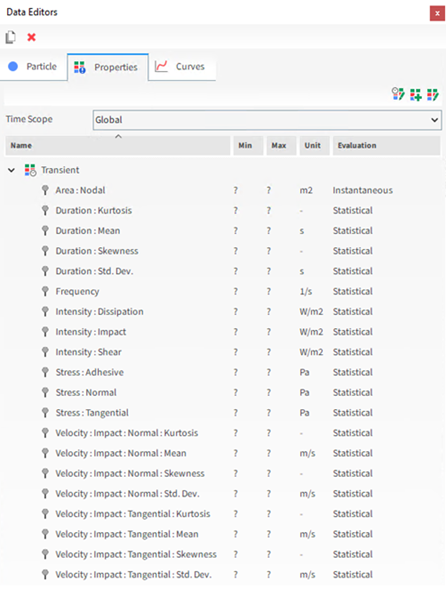
Table 5: Properties available for an individual Particle set that supports the collection of Intra-particle Collision Statistics
Property Name | Description |
|---|---|
Area : Nodal | When the Intra-particle Collisions Statistic module is enabled (see also About Intra-Particle Collision Statistics), this provides the surface area making up the different regions of influence surrounding the vertices of the representative particle of the selected particle set. This is useful for defining custom properties, such as frequency / area, intensity area, and so on. See also the "Collision statistics" section of the DEM Technical Manual (from the Rocky Help menu, point to Manuals, and then click DEM Technical Manual). |
Duration : Kurtosis | When the Duration option is enabled on the Intra-particle Collision Statistics module (see also About Intra-Particle Collision Statistics), this provides the kurtosis value of the duration of the collisions recorded in different regions of the representative particle of the selected particle set, during an interval between two consecutive output time. The kurtosis is a measure of how tall and sharp the central peak of a statistical distribution is. See also the "Collision statistics" section of the DEM Technical Manual (from the Rocky Help menu, point to Manuals, and then click DEM Technical Manual). |
Duration : Mean | When the Duration option is enabled on the Intra-particle Collision Statistics module (see also About Intra-Particle Collision Statistics), this provides the mean value of the duration of the collisions recorded in different regions of the representative particle of the selected particle set, during an interval between two consecutive output times. See also the "Collision statistics" section of the DEM Technical Manual (from the Rocky Help menu, point to Manuals, and then click DEM Technical Manual). |
Duration : Skewness | When the Duration option is enabled on the Intra-particle Collision Statistics module (see also About Intra-Particle Collision Statistics), this provides the skewness value of the duration of the collisions recorded in different regions of the representative particle of the selected particle set, during an interval between two consecutive output times. The skewness is a measure of the asymmetry of a statistical distribution about its mean. See also the "Collision statistics" section of the DEM Technical Manual (from the Rocky Help menu, point to Manuals, and then click DEM Technical Manual). |
Duration : Std. Dev. | When the Duration option is enabled on the Intra-particle Collision Statistics module (see also About Intra-Particle Collision Statistics), this provides the standard deviation value of the duration of the collisions recorded in different regions of the representative particle of the selected particle set, during an interval between two consecutive output times. See also the "Collision statistics" section of the DEM Technical Manual (from the Rocky Help menu, point to Manuals, and then click DEM Technical Manual). |
Frequency | When the Frequency option is enabled on the Intra-particle Collision Statistics module (see also About Intra-Particle Collision Statistics), this provides the average collision frequency per particle recorded in different regions of the representative particle of the selected particle set, during an interval between two consecutive output times. See also the "Collision statistics" section of the DEM Technical Manual (from the Rocky Help menu, point to Manuals, and then click DEM Technical Manual). |
Intensity : Dissipation | When the Intensities option is enabled on the Intra-particle Collision Statistics module (see also About Intra-Particle Collision Statistics), this provides the average power dissipated per unit area by the contact forces resulting from the collisions recorded in different regions of the representative particle of the selected particle set, during an interval between two consecutive output times. See also the "Collision statistics" section of the DEM Technical Manual (from the Rocky Help menu, point to Manuals, and then click DEM Technical Manual). |
Intensity : Impact | When the Intensities option is enabled on the Intra-particle Collision Statistics module (see also About Intra-Particle Collision Statistics), this provides the average impact power divided by the area made by the contact forces resulting from the collisions recorded in different regions of the representative particle of the selected particle set, during an interval between two consecutive output times. |
Intensity : Shear | When the Intensities option is enabled on the Intra-particle Collision Statistics module (see also About Intra-Particle Collision Statistics), this provides the average shear power made by the contact forces resulting from the collisions, the average shear power by area recorded in different regions of the representative particle of the selected particle set, during an interval between two consecutive output times. |
Stress : Adhesive | When the Stresses option is enabled on the Intra-particle Collision Statistics module (see also About Intra-Particle Collision Statistics), an Adhesive Force model (other than None) is enabled (see also About Physics Parameters), and an Adhesive Force Fraction for a particle-boundary and/or particle-particle Materials Interaction pair has a value set higher than zero (see also About Modifying Materials Interactions and Adhesion Values), this provides the average adhesive stress resulting from the collisions recorded in different regions of the representative particle of the selected particle set, during an interval between two consecutive output times. See also the "Collision statistics" section of the DEM Technical Manual (from the Rocky Help menu, point to Manuals, and then click DEM Technical Manual). |
Stress : Normal | When the Stresses option is enabled on the Intra-particle Collision Statistics module (see also About Intra-Particle Collision Statistics), this provides the average normal stress resulting from the collisions recorded in different regions of the representative particle of the selected particle set, during an interval between two consecutive output times. See also the "Collision statistics" section of the DEM Technical Manual (from the Rocky Help menu, point to Manuals, and then click DEM Technical Manual). |
Stress : Tangential | When the Stresses option is enabled on the Intra-particle Collision Statistics module (see also About Intra-Particle Collision Statistics), this provides the average tangential stress resulting from the collisions recorded in different regions of the representative particle of the selected particle set, during an interval between two consecutive output times. See also the "Collision statistics" section of the DEM Technical Manual (from the Rocky Help menu, point to Manuals, and then click DEM Technical Manual). |
Velocity : Impact : Normal : Kurtosis | When the Normal Impact Velocity option is enabled on the Intra-particle Collision Statistics module (see also About Intra-Particle Collision Statistics), this provides the kurtosis value of the impact relative velocity in the normal direction resulting from the collisions recorded in different regions of the representative particle of the selected particle set, during an interval between two consecutive output times. The kurtosis is a measure of how tall and sharp the central peak of a statistical distribution is. See also the "Collision statistics" section of the DEM Technical Manual (from the Rocky Help menu, point to Manuals, and then click DEM Technical Manual). |
Velocity : Impact : Normal : Mean | When the Normal Impact Velocity option is enabled on the Intra-particle Collision Statistics module (see also About Intra-Particle Collision Statistics), this provides the mean value of the impact relative velocity in the normal direction resulting from the collisions recorded in different regions of the representative particle of the selected particle set, during an interval between two consecutive output times. See also the "Collision statistics" section of the DEM Technical Manual (from the Rocky Help menu, point to Manuals, and then click DEM Technical Manual). |
Velocity : Impact : Normal : Skewness | When the Normal Impact Velocity option is enabled on the Intra-particle Collision Statistics module (see also About Intra-Particle Collision Statistics), this provides the skewness value of the impact relative velocity in the normal direction resulting from the collisions recorded in different regions of the representative particle of the selected particle set, during an interval between two consecutive output times. The skewness is a measure of the asymmetry of a statistical distribution about its mean. See also the "Collision statistics" section of the DEM Technical Manual (from the Rocky Help menu, point to Manuals, and then click DEM Technical Manual). |
Velocity : Impact : Normal : Std. Dev. | When the Normal Impact Velocity option is enabled on the Intra-particle Collision Statistics module (see also About Intra-Particle Collision Statistics), this provides the standard deviation value of the impact relative velocity in the normal direction resulting from the collisions recorded in different regions of the representative particle of the selected particle set, during an interval between two consecutive output times. See also the "Collision statistics" section of the DEM Technical Manual (from the Rocky Help menu, point to Manuals, and then click DEM Technical Manual). |
Velocity : Impact : Tangential : Kurtosis | When the Tangential Impact Velocity option is enabled on the Intra-particle Collision Statistics module (see also About Intra-Particle Collision Statistics), this provides the kurtosis value of the impact relative velocity in the tangential direction resulting from the collisions recorded in different regions of the representative particle of the selected particle set, during an interval between two consecutive output times. The kurtosis is a measure of how tall and sharp the central peak of a statistical distribution is. See also the "Collision statistics" section of the DEM Technical Manual (from the Rocky Help menu, point to Manuals, and then click DEM Technical Manual). |
Velocity : Impact : Tangential : Mean | When the Tangential Impact Velocity option is enabled on the Intra-particle Collision Statistics module (see also About Intra-Particle Collision Statistics), this provides the mean value of the impact relative velocity in the tangential direction resulting from the collisions recorded in different regions of the representative particle of the selected particle set, during an interval between two consecutive output times. See also the "Collision statistics" section of the DEM Technical Manual (from the Rocky Help menu, point to Manuals, and then click DEM Technical Manual). |
Velocity : Impact : Tangential : Skewness | When the Tangential Impact Velocity option is enabled on the Intra-particle Collision Statistics module (see also About Intra-Particle Collision Statistics), this provides the skewness value of the impact relative velocity in the tangential direction resulting from the collisions recorded in different regions of the representative particle of the selected particle set, during an interval between two consecutive output times. The skewness is a measure of the asymmetry of a statistical distribution about its mean. See also the "Collision statistics" section of the DEM Technical Manual (from the Rocky Help menu, point to Manuals, and then click DEM Technical Manual). |
Velocity : Impact : Tangential : Std. Dev. | When the Tangential Impact Velocity option is enabled on the Intra-particle Collision Statistics module (see also About Intra-Particle Collision Statistics), this provides the standard deviation value of the impact relative velocity in the tangential direction resulting from the collisions recorded in different regions of the representative particle of the selected particle set, during an interval between two consecutive output times. See also the "Collision statistics" section of the DEM Technical Manual (from the Rocky Help menu, point to Manuals, and then click DEM Technical Manual). |
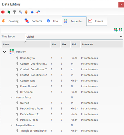
Table 6: Properties available by default when Contacts data is collected
Property Name | Description |
|---|---|
Absolute Normal Force | The current normal force magnitude of the contact. |
Boundary To | Identifies the parent entity of the object being contacted and for boundaries specifically, identifies the specific component. No matter whether they have sustained contacts or not, the list always includes all geometry components and inlets, numbered from 0 (zero) in (roughly) the order in which they were added. It also includes the main Particle category (representing all Particle Group), which will always be displayed as -1. Tip: The numbers are needed, in part, when creating a Property User Process (see also About the Property User Process). Use the Color scale to map the numbers to the object name (see also About Color Scales). |
Contact Type | The type of contact being made. Specifically:
|
Contact : Coordinate : X | The coordinate location of the contact along the X-axis. |
Contact : Coordinate : Y | The coordinate location of the contact along the Y-axis. |
Contact : Coordinate : Z | The coordinate location of the contact along the Z-axis. |
Initial Contact Overlap | The initial magnitude of the contact overlap between the contact pair (particle-particle or particle boundary). |
Is Frictional | Indicates whether the contact is frictional and adhesive, or only adhesive. Specifically:
|
Force : Normal : X | The current normal force of the contact in the X direction. |
|
Force : Normal : Y | The current normal force of the contact in the Y direction. |
|
Force : Normal : Z | The current normal force of the contact in the Z direction. |
Overlap | The current magnitude of the contact overlap between the contact pair (particle-particle or particle boundary). |
Particle Group From | Displays the name of the Particle Group doing the contacting. Note: In Rocky, the object doing the contact is always a particle. Even if a boundary in motion collides with a particle, Rocky still considers the particle as the originator of the contact. |
Particle Group To | Identifies the parent entity of the object being contacted and for Particles specifically, identifies the specific Particle Group being contacted. No matter whether they have sustained contacts or not, the list always includes all Particle sets, numbered from 0 (zero) in (roughly) the order in which they were added. It also includes the main Boundary category (representing all geometry components and inlets), which will always be displayed as -1. Tip: The numbers are needed, in part, when creating a Property User Process (see also About the Property User Process). Use the Color scale to map the numbers to the object name (see also About Color Scales). |
Particle ID From | Displays the unique identifier (particle ID) associated with the particle doing the contacting. Note: In Rocky, the object doing the contact is always a particle. Even if a boundary in motion collides with a particle, Rocky still considers the particle as the originator of the contact. |
|
Force : Tangential : X | The current tangential force of the contact in the X direction. |
Force : Tangential : Y | The current tangential force of the contact in the Y direction. |
Force : Tangential : Z | The current tangential force of the contact in the Z direction. |
Triangle or Particle ID To | Displays the unique identifier (ID) associated with the cell being contacted. Specifically:
|
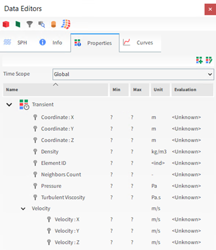
Table 7: Properties available when running a SPH simulation
Property Name | Description |
|---|---|
|
Coordinate : X |
The Coordinate component in the X direction for each SPH element. |
|
Coordinate : Y |
The Coordinate component in the Y direction for each SPH element. |
|
Coordinate : Z |
The Coordinate component in the Z direction for each SPH element. |
|
Density |
The density of each SPH element |
|
Element ID |
The numeric identifier unique to each individual whole SPH element. |
|
Neighbors Count |
Count of neighbors SPH elements. |
Pressure | The pressure that each SPH element is subjected to. |
|
Temperature |
Temperature of SPH elements. |
Turbulent Viscosity (only available if a turbulence model is enabled) | The turbulent viscosity associated to each SPH element |
Velocity : X | The velocity vector component in the X direction for each SPH element. |
Velocity : Y | The velocity vector component in the Y direction for each SPH element. |
Velocity : Z | The velocity vector component in the Z direction for each SPH element. |
(See also About Contacts).
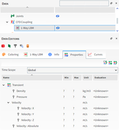
Table 8: Properties available by default for 1-Way LBM (CFD Coupling)
Property Name | Description |
|---|---|
Density | The density the fluid. |
Pressure | The pressure at each individual fluid node. |
Velocity | The velocity vector of each individual fluid node, the magnitude of which is made up of the x, y, and z components respectively. Note: Because this is a vector, display is limited to the 3D View only. |
Velocity : X | The x-component of the fluid velocity in global coordinates. |
Velocity : Y | The y-component of the fluid velocity in global coordinates. |
Velocity : Z | The z-component of the fluid velocity in global coordinates. |
|
Velocity : Absolute |
The absolute velocity of each individual fluid node. |
(See also About Using the 1-Way LBM Method.)
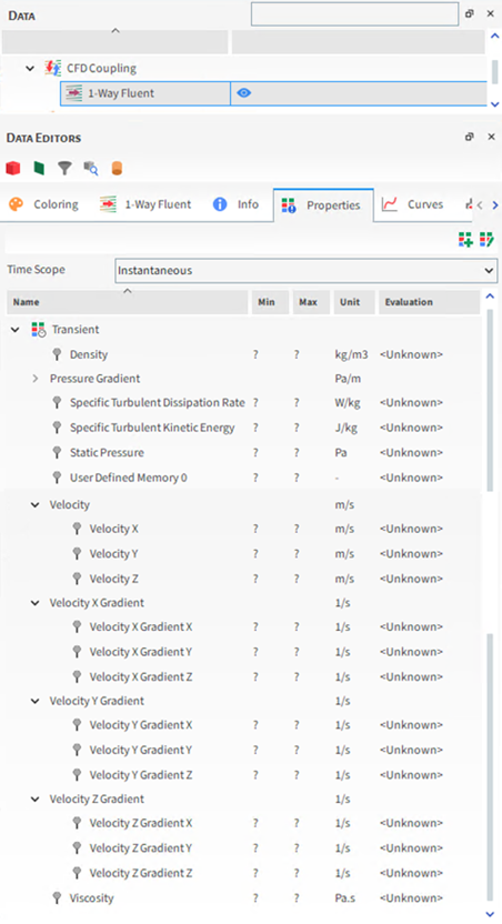
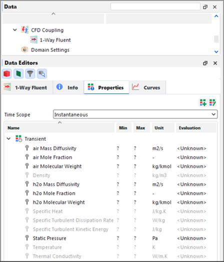
Table 9: Properties available by default for 1-Way Fluent (CFD Coupling)
Property Name | Description |
|---|---|
Density | The density of the fluid. For multiphase flows, the mixture density is reported. |
Pressure | The static pressure of the fluid. |
Pressure Gradient | The pressure gradient of the fluid, the magnitude of which is made up of the x, y, and z components respectively. |
Pressure Gradient X | The pressure gradient of the fluid in the X direction. |
Pressure Gradient Y | The pressure gradient of the fluid in the Y direction. |
Pressure Gradient Z | The pressure gradient of the fluid in the Z direction. |
Specific Turbulent Dissipation Rate | When the .f2r file has a turbulent model that uses turbulence dissipation rate as one of its quantities, this is the specific turbulent dissipation rate of the fluid. |
Specific Turbulent Kinetic Energy | When the .f2r file has a turbulent model that uses turbulence kinetic energy as one of its quantities, this is the specific turbulent kinetic energy of the fluid. |
Specific Heat | When Thermal Model is enabled (see also Enable Thermal Modeling) and the Fluent case has a thermal solution, this is the specific heat of the fluid. For multiphase flows, the specific heat of the mixture is reported. |
Temperature | When Thermal Model is enabled (see also Enable Thermal Modeling) and the Fluent case has a thermal solution, this is the thermodynamic temperature of the fluid. |
Thermal Conductivity | When Thermal Model is enabled (see also Enable Thermal Modeling) and the Fluent case has a thermal solution, this is the thermal conductivity of the fluid. For multiphase flows, the thermal conductivity of the mixture is reported. |
Velocity | The velocity vector of the fluid, the magnitude of which is made up of the x, y, and z components respectively. Note: Because this is a vector, display is limited to the 3D View only. |
Velocity X | The velocity of the fluid along the X-axis. |
Velocity Y | The velocity of the fluid along the Y-axis. |
Velocity Z | The velocity of the fluid along the Z-axis. |
Velocity X Gradient | The gradient of the velocity of the fluid along the X-axis. |
Velocity X Gradient X | The gradient of the X Velocity in the X direction. |
Velocity X Gradient Y | The gradient of the X Velocity in the Y direction. |
Velocity X Gradient Z | The gradient of the X Velocity in the Z direction. |
Velocity Y Gradient | The gradient of the velocity of the fluid along the Y-axis. |
Velocity Y Gradient X | The gradient of the Y Velocity in the X direction. |
Velocity Y Gradient Y | The gradient of the Y Velocity in the Y direction. |
Velocity Y Gradient Z | The gradient of the Y Velocity in the Z direction. |
Velocity Z Gradient | The gradient of the velocity of the fluid along the Z-axis. |
Velocity Z Gradient X | The gradient of the Z Velocity in the X direction. |
Velocity Z Gradient Y | The gradient of the Z Velocity in the Y direction. |
Velocity Z Gradient Z | The gradient of the Z Velocity in the Z direction. |
Viscosity | The viscosity of the fluid. For multiphase flows, the viscosity of the mixture is reported. |
(See also About Using the 1-Way Fluent Method).
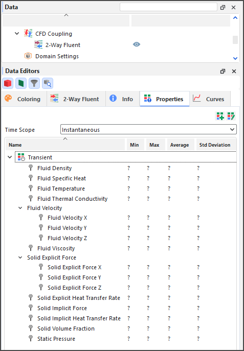
Table 10: Properties available by default for 2-Way Fluent
Property Name | Description |
|---|---|
Fluid Density | The density of the fluid. For multiphase flows, the density o the mixture is reported. |
Fluid Specific Heat | When Thermal Model is enabled (see also Enable Thermal Modeling) and the Fluent case has a thermal solution, this is the specific heat of the fluid. For multiphase flows, the specific heat of the mixture is reported. |
Fluid Temperature | When Thermal Model is enabled (see also Enable Thermal Modeling) and the Fluent case has a thermal solution, this is the thermodynamic temperature of the fluid. |
Fluid Thermal Conductivity | When Thermal Model is enabled (see also Enable Thermal Modeling) and the Fluent case has a thermal solution, this is the thermal conductivity of the fluid. For multiphase flows, the thermal conductivity of the mixture is reported. |
Fluid Turbulent Dissipation Rate | When the Fluent case has a turbulent model that uses turbulence dissipation as one of its quantities, this is the turbulent dissipation rate of the fluid. |
Fluid Turbulent Kinetic Energy | When the Fluent case has a turbulent model that uses turbulence kinetic energy as one of its quantities, this is the turbulent kinetic energy of the fluid. |
Fluid Velocity | The velocity vector of the fluid, the magnitude of which is made up of the x, y, and z components respectively. Note: Because this is a vector, display is limited to the 3D View only. |
Fluid Velocity X | The velocity of the fluid in the x direction. |
Fluid Velocity Y | The velocity of the fluid in the y direction. |
Fluid Velocity Z | The velocity of the fluid in the z direction. |
Fluid Viscosity | The viscosity of the fluid. For multiphase flows, the viscosity of the mixture is reported. |
Solid Explicit Force | The explicit portion of the total momentum contribution from particle-fluid interaction forces, which is in turn given by:
where:
Notes:
|
Solid Explicit Force X | The explicit momentum source added to the fluid momentum equation in the x direction. |
Solid Explicit Force Y | The explicit momentum source added to the fluid momentum equation in the y direction. |
Solid Explicit Force Z | The explicit momentum source added to the fluid momentum equation in the z direction. |
Solid Explicit Heat Transfer Rate | When Thermal Model is enabled (see also Enable Thermal Modeling) and the Fluent case has a thermal solution, this is the explicit heat transfer rate source contribution of the particles into the fluid, where the total heat source is given by:
where:
|
Solid Implicit Force | The implicit portion of the total momentum contribution from particle-fluid interaction forces, which is in turn given by:
where:
See also I cannot find the directional properties for Solid Implicit Force. |
Solid Implicit Heat Transfer Rate | When Thermal Model is enabled (see also Enable Thermal Modeling) and the Fluent case has a thermal solution, this is the implicit heat transfer rate source contribution of the particles into the fluid, where the total heat source is given by:
where:
|
Solid Volume Fraction | The ratio between the summation of the particle volumes within a CFD cell and the volume of the cell. |
Static Pressure | The static pressure of the fluid. |


(See also About Using the 2-Way Fluent Method).
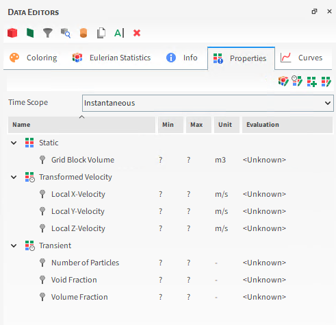
Table 11: Properties available by default for Eulerian Statistics
Property Name | Description |
|---|---|
Grid Block Volume | The total volume of each individual block the Cube or Cylinder User Process is divided into (see also About Eulerian Statistics). |
Stress Component <Various> |
Important: To obtain this property, you must first have enabled the Collect Contacts Data checkbox on the Contacts entity prior to processing your simulation (see also About Contacts). The stress tensor for each Eulerian bin is computed as described in the Stress Tensor definition (below). Each one of the six independent components represents the average stress tensor resulting from particles' contact with other particles or boundaries. As this is a second order symmetric tensor, three of these values represent normal stresses and three represent shear stresses. Stress components are given in a coordinate system based upon the User Process shape from which the Eulerian Statistics User Process is created. Specifically:
For both Cubes and Cylinders, this follows the conventional index notation
(as shown below), whereby stress components have two different subscript
indices that vary among X, Y, and Z for Cubes, and R,
A stress component is positive if it acts in the positive direction of the
coordinate axes, and if the plane where it acts has an outward normal vector
pointing in the positive coordinate direction. This gives the nine components,
but since the stress matrix is symmetric, i.e. As an example, in the case of an Eulerian Statistics User Process being applied to a Cube User Process, the stress component YZ indicates the stress on the face whose normal is in the Y direction and acting in the Z direction. |
Transformed Velocity | The transformed velocity of each Eulerian bin is computed as:
where:
|
Local X-Velocity | For Cube User Processes, this is the bin velocity in the local X direction (red directional handle) relative to the Cube, computed based upon the Transformed Velocity description (above). |
Local Y-Velocity | For Cube User Processes, this is the bin velocity in the local Y direction (green directional handle) relative to the Cube, computed based upon the Transformed Velocity description (above). |
Local Z-Velocity | For Cube User Processes, this is the bin velocity in the local Z direction (blue directional handle) relative to the Cube, computed based upon the Transformed Velocity description (above). |
Local R-Velocity | For Cylinder User Processes, this is the particle speed in the radial direction relative to the Cylinder, computed based upon the Transformed Velocity description (above). |
Local T-Velocity | For Cylinder User Processes, this is the particle speed in the tangential direction relative to the Cylinder, computed based upon the Transformed Velocity description (above). |
Local Z-Velocity | For Cylinder User Processes, this is the particle speed in the axial direction relative to the Cylinder, computed based upon the Transformed Velocity description (above). |
First Stress Invariant | Important: To obtain this property, you must first have enabled the Collect Contacts Data checkbox on the Contacts entity prior to processing your simulation (see also About Contacts). Also known as "trace," this is the is the sum of the diagonal stress components, as given by the following equation:
|
Number of Particles | The amount of particles in each individual block the Cube or Cylinder User Process is divided into (see also About Eulerian Statistics). |
Second Stress Invariant | Important: To obtain this property, you must first have enabled the Collect Contacts Data checkbox on the Contacts entity prior to processing your simulation (see also About Contacts). The sum of the principal minors as given by the following equation:
|
Stress Tensor | Important: To obtain this property, you must first have enabled the Collect Contacts Data checkbox on the Contacts entity prior to processing your simulation (see also About Contacts). The average stress tensor for the bin is computed as:
where:
|
Third Stress Invariant | Important: To obtain this property, you must first have enabled the Collect Contacts Data checkbox on the Contacts entity prior to processing your simulation (see also About Contacts). The determinant of the stress tensor, as given by the following equation:
|
Transformed Stress Tensor | Important: To obtain this property, you must first have enabled the Collect Contacts Data checkbox on the Contacts entity prior to processing your simulation (see also About Contacts). The stress tensor using the local coordinates of the Cylinder or Cube User Process upon which the Eulerian Statistics User Process was created. |
Void Fraction | Also known as porosity, this is the ratio between the volume of the block not occupied by particles divided by the volume of the block itself, according to the following equation:
where:
Tip: Void Fraction = 1 - Volume Fraction |
Volume Fraction | The ratio between the total particle volume inside the block divided by the volume of the block itself, according to the following equation:
where:
Volume Fraction represents the volume of the block occupied by particles. Since it takes into account the sum of the volume of all particles that have nodes located inside the corresponding block, it can return values above 1 in cases where the ratio between the particle size and the block volume is small. Tip: Void Fraction = 1 - Volume Fraction |


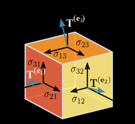


What would you like to do?
See Also:
Unlike Properties, which record many individual values for each output time, the Curves tab displays only the entity properties that produce a single value. This means that a Property becomes a Curve after its data set is reduced to a single value; for example, by choosing to sum all the values or average them out.
Curves are calculated using Global coordinates and are collected for geometry components, including conveyors and imported geometries, as well as for Particles, the Solver, and individual Motion Frames. And as with Properties, individual User Processes linked to any entities with Curve properties will also display the same properties on their own Curves tabs.
Unlike Properties, you cannot display Curves in a 3D View or a Histogram due to the one-dimensional aspect of the data that is recorded. The ways in which you can display Curves in the Rocky UI are described in the table below.
Table 1: Methods for Displaying Curves data
Display Options | Method | See Also |
|---|---|---|
Through the Curves tab | From the property, choose to Compute Statistics and then use the UI to display the individual values you want. | |
In a Time Plot | Create a Time Plot from the property. |
In Rocky, both imported Geometries and Motion Frames have Curves properties available, both of which provide translational and angular velocities in different directions. At first glance, it might appear that the velocity values for an imported geometry might be equal to those of the Motion Frame assigned to it, but this is not always the case, as described below and illustrated in Figure 5.18: Diagram showing how Motion Frames assigned to a rectangular boundary affect the resulting velocity Curves for the boundary
In cases where the Motion Frame assigned to the geometry has only translation motions, the boundary velocities will be equal to that of the Motion Frame.
In cases where the Motion Frame assigned to the geometry has only rotation motions, the boundary will have the same angular velocity as the Motion Frame plus a separate translational velocity as given by the angular velocity of the frame and the distance between the boundary and the frame (see Figure 1).
In cases where the Motion Frame assigned to the geometry has both translation and rotation motions, the boundary will have the same angular velocity and a combination of the frame's translational velocity and the additional translational velocity applied due to the frame's rotation and the distance between the boundary and the frame.
Figure 5.18: Diagram showing how Motion Frames assigned to a rectangular boundary affect the resulting velocity Curves for the boundary
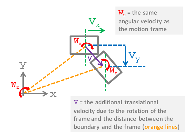
(See also About Creating and Applying Motion Frames and I cannot find some Properties or Curves in this version of Rocky).
See the images and tables below to learn about the various Curves available in Rocky.
(See also About Collision Statistics for Boundaries)
Figure 5.19: Geometry (Feed; Receiving; Imported) Curves options on the Data Editors panel when Boundary Collision Statistics are collected
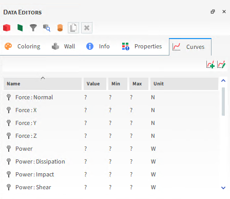
Figure 5.20: Imported Geometry, Curves options on the Data Editors panel when Motion Frames are assigned
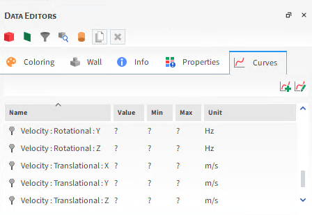
(See also About Creating and Applying Motion Frames and I cannot find some Properties or Curves in this version of Rocky.)
Table 2: Curves options for Geometries (Feed Conveyors, Receiving Conveyors, and Imported)
Function | Description |
|---|---|
All Geometries When Boundary Collision Statistics are collected Tip: See also About Collision Statistics for Boundaries. | |
Force : Normal | When the Stresses option is enabled on the Boundary Collision Statistics module (see also About Collision Statistics for Boundaries), this provides the sum of the normal forces acting on all the triangles that make up a geometry surface. This is useful for measuring the degree of upwards belt misalignment. |
Force : X | When the Forces for FEM Analysis option is enabled on the Boundary Collision Statistics module (see also About Collision Statistics for Boundaries), this provides the force applied to the geometry along the X axis. This is useful for measuring the degree of belt misalignment in the X direction. |
Force : Y | When the Forces for FEM Analysis option is enabled on the Boundary Collision Statistics module (see also About Collision Statistics for Boundaries), this provides the force applied to the geometry along the Y axis. This is useful for measuring the degree of belt misalignment in the Y direction. |
Force : Z | When the Forces for FEM Analysis option is enabled on the Boundary Collision Statistics module (see also About Collision Statistics for Boundaries), this provides the force applied to the geometry along the Z axis. This is useful for measuring the degree of belt misalignment in the Z direction. |
Power | When the Intensities option is enabled on the Boundary Collision Statistics module (see also About Collision Statistics for Boundaries), this provides the power required to move the geometry at the specified speed given the particle load applied to the surface. This is useful for determining the power applied by the geometry. |
Power : Dissipation | When the Intensities option is enabled on the Boundary Collision Statistics module (see also About Collision Statistics for Boundaries), this provides the power dissipated in the collisions against a geometry surface by the contact forces. This is useful for determining the amount of mechanical energy that is transformed irreversibly into other forms of energy during a collision. |
Power : Impact | When the Intensities option is enabled on the Boundary Collision Statistics module (see also About Collision Statistics for Boundaries), this provides the power transferred during the loading phase of all collisions against the geometry surface. It is related to the normal component of the contact force, and it is useful for determining how particle impact affects the surface |
Power : Shear | When the Intensities option is enabled on the Boundary Collision Statistics module (see also About Collision Statistics for Boundaries), this provides the power transferred during the unloading phase of all collisions against the geometry surface. This is useful for predicting the abrasive wear of surface boundaries. |
Imported Geometries Only When Motion Frames are assigned Tip:See additional information in the About Curves for Imported Geometries and Motion Frames section above | |
Velocity : Rotational : X | When the geometry has a Motion Frame assigned to it (see also About Creating and Applying Motion Frames to Custom Geometries), this is the rotational (angular) velocity of the assigned Motion Frame as defined in the X direction. |
Velocity : Rotational : Y | When the geometry has a Motion Frame assigned to it (see also About Creating and Applying Motion Frames to Custom Geometries), this is the rotational (angular) velocity of the assigned Motion Frame as defined in the Y direction. |
Velocity : Rotational : Z | When the geometry has a Motion Frame assigned to it (see also About Creating and Applying Motion Frames to Custom Geometries), this is the rotational (angular) velocity of the assigned Motion Frame as defined in the Z direction. |
Velocity : Translational : X | When the geometry has a Motion Frame assigned to it (see also About Creating and Applying Motion Frames to Custom Geometries), this is the translational velocity of the assigned Motion Frame as defined in the X direction. |
Velocity : Translational : Y | When the geometry has a Motion Frame assigned to it (see also About Creating and Applying Motion Frames to Custom Geometries), this is the translational velocity of the assigned Motion Frame as defined in the Y direction. |
Velocity : Translational : Z | When the geometry has a Motion Frame assigned to it (see also About Creating and Applying Motion Frames to Custom Geometries), this is the translational velocity of the assigned Motion Frame as defined in the Z direction. |
Notes:
Curves related to particle breakage are applicable only for simulations with Instantaneous Breakage.
For most Curves, a point in an output time represents what happened in the interval between that output time and the previous one.
(See also About Adding and Editing Particle Sets.)
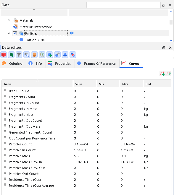
Table 3: Standard Curves options for Particles
Function | Description |
|---|---|
Breaks Count | When Instantaneous Breakage parameters are set, this provides the total number of individual whole particles and fragments that broke during an interval between two consecutive output times. |
Fragments Count | When Instantaneous Breakage parameters are set, this provides the total number of fragments that are currently in the selection. |
Fragments In Count | When Instantaneous Breakage parameters are set, this provides the total number of particle fragments that entered the selection during an interval between two consecutive output times. |
Fragments In Mass | When Instantaneous Breakage parameters are set, this provides the total mass of particle fragments that have entered the selection during an interval between two consecutive output times. |
Fragments Mass | When Instantaneous Breakage parameters are set, this provides the total mass of the particle fragments that are currently within the selection. |
Fragments Out Count | When Instantaneous Breakage parameters are set, this provides the total number of particle fragments that have exited the selection during an interval between two consecutive output times. |
Fragments Out Mass | When Instantaneous Breakage parameters are set, this provides the total mass of particle fragments that have exited the selection during an interval between two consecutive output times. |
Generated Fragments Count | When Instantaneous Breakage parameters are set, this provides the total number of new particle fragments that were generated inside the selection during an interval between two consecutive output times. |
Out Count per Residence Time | For each point in the curve, the vertical coordinate indicates the total number of whole particles and fragments inside the selection that have spent the time represented by the horizontal coordinate. |
Particles Count | The total number of whole particles and particle fragments that are currently in the selection. |
Particles In Count | The total number of whole particles and particle fragments that have entered the selection during an interval between two consecutive output times. |
Particles Mass Flow In | The mass flow of particles and fragments entering the selection in a given simulation output. |
Particles Mass | The total mass of whole particles and fragments that are currently in the selection. |
Particles Out Count | The total number of whole particles and fragments that have exited the selection during an interval between two consecutive output times. |
Particles Mass Flow Out | The mass flow of particles and fragments exiting the selection in a given simulation output. |
Residence Time (Out) | For any whole particles or fragments that have exited the selection during an interval between two consecutive output times, this is the average amount of time that they were inside the selection boundaries before exiting. |
Residence Time (Out) Average | For all whole particles and fragments that have exited the selection prior to the last fully calculated output time, this is the average (but cumulative) amount of time that they were inside the simulation boundaries before exiting. |
(See also About Inter-group Collision Statistics.)
Figure 5.22: Particles, Curves options on the Data Editors panel when Inter-group Collision Statistics is enabled
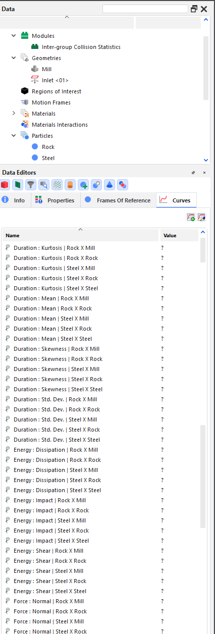
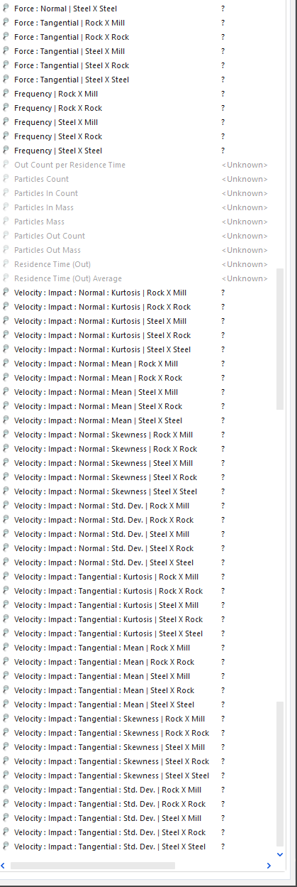
Note: For all Inter-group Collisions Statistics curves, the effects of upscaling will be ignored for any meshed particles with Meshed Particles Upscaling enabled. (See also About Meshed Particles Upscaling).
Table 4: Additional Curves options for Particles when Inter-group Collision Statistics is enabled
Function | Description |
|---|---|
Duration : Kurtosis | When the Duration option is enabled on the Inter-group Collision Statistics module (see also About Inter-group Collision Statistics), this provides the kurtosis value of the duration of all collisions recorded for the indicated pair (particle-particle or particle-geometry) that occurred during an interval between two consecutive output time. The kurtosis is a measure of how tall and sharp the central peak of a statistical distribution is. See also the "Collision statistics" section of the DEM Technical Manual (from the Rocky Help menu, point to Manuals, and then click DEM Technical Manual). |
Duration : Mean | When the Duration option is enabled on the Inter-group Collision Statistics module (see also About Inter-group Collision Statistics), this provides the mean value of the duration of all collisions recorded for the indicated pair (particle-particle or particle-geometry) that occurred during an interval between two consecutive output times. See also the "Collision statistics" section of the DEM Technical Manual (from the Rocky Help menu, point to Manuals, and then click DEM Technical Manual). |
Duration : Skewness | When the Duration option is enabled on the Inter-group Collision Statistics module (see also About Inter-group Collision Statistics), this provides the skewness value of the duration of all collisions recorded for the indicated pair (particle-particle or particle-geometry) that occurred during an interval between two consecutive output times. The skewness is a measure of the asymmetry of a statistical distribution about its mean. See also the "Collision statistics" section of the DEM Technical Manual (from the Rocky Help menu, point to Manuals, and then click DEM Technical Manual). |
Duration : Std. Dev. | When the Duration option is enabled on the Inter-group Collision Statistics module (see also About Inter-group Collision Statistics), this provides the standard deviation value of the duration of all collisions recorded for the indicated pair (particle-particle or particle-geometry) that occurred during an interval between two consecutive output times. See also the "Collision statistics" section of the DEM Technical Manual (from the Rocky Help menu, point to Manuals, and then click DEM Technical Manual). |
Energy : Dissipation | When the Energy Dissipation option is enabled on the Inter-group Collision Statistics module (see also About Inter-group Collision Statistics), this provides the total energy dissipated for all collisions recorded for the indicated pair (particle-particle or particle-geometry) that occurred during an interval between two consecutive output times. See also the "Collision statistics" section of the DEM Technical Manual (from the Rocky Help menu, point to Manuals, and then click DEM Technical Manual). |
Energy : Impact | When the Impact Energy option is enabled on the Inter-group Collision Statistics module (see also About Inter-group Collision Statistics), this provides the total impact energy for all collisions recorded for the indicated pair (particle-particle or particle-geometry) that occurred during an interval between two consecutive output times. See also the "Collision statistics" section of the DEM Technical Manual (from the Rocky Help menu, point to Manuals, and then click DEM Technical Manual). |
Energy : Shear | When the Shear Energy option is enabled on the Inter-group Collision Statistics module (see also About Inter-group Collision Statistics), this provides the total shear energy for all collisions recorded for the indicated pair (particle-particle or particle-geometry) that occurred during an interval between two consecutive output times. See also the "Collision statistics" section of the DEM Technical Manual (from the Rocky Help menu, point to Manuals, and then click DEM Technical Manual). |
Force : Normal | When the Forces option is enabled on the Inter-group Collision Statistics module (see also About Inter-group Collision Statistics), this provides the total force in the normal direction for all collisions recorded for the indicated pair (particle-particle or particle-geometry) that occurred during an interval between two consecutive output times. See also the "Collision statistics" section of the DEM Technical Manual (from the Rocky Help menu, point to Manuals, and then click DEM Technical Manual). |
Force : Tangential | When the Forces option is enabled on the Inter-group Collision Statistics module (see also About Inter-group Collision Statistics), this provides the total force in the tangential direction for all collisions recorded for the indicated pair (particle-particle or particle-geometry) that occurred during an interval between two consecutive output times. See also the "Collision statistics" section of the DEM Technical Manual (from the Rocky Help menu, point to Manuals, and then click DEM Technical Manual). |
Frequency | When the Frequency option is enabled on the Inter-group Collision Statistics module (see also About Inter-group Collision Statistics), this provides the total collision frequency for all collisions recorded for the indicated pair (particle-particle or particle-geometry) that occurred during an interval between two consecutive output times. See also the "Collision statistics" section of the DEM Technical Manual (from the Rocky Help menu, point to Manuals, and then click DEM Technical Manual). |
Velocity : Impact : Normal : Kurtosis | When the Normal Impact Velocity option is enabled on the Inter-group Collision Statistics module (see also About Inter-group Collision Statistics), this provides the kurtosis value of the impact relative velocity in normal direction for all collisions recorded for the indicated pair (particle-particle or particle-geometry) that occurred during an interval between two consecutive output times. The kurtosis is a measure of how tall and sharp the central peak of a statistical distribution is. See also the "Collision statistics" section of the DEM Technical Manual (from the Rocky Help menu, point to Manuals, and then click DEM Technical Manual). |
Velocity : Impact : Normal : Mean | When the Normal Impact Velocity option is enabled on the Inter-group Collision Statistics module (see also About Inter-group Collision Statistics), this provides the mean value of the impact relative velocity in normal direction for all collisions recorded for the indicated pair (particle-particle or particle-geometry) that occurred during an interval between two consecutive output times. See also the "Collision statistics" section of the DEM Technical Manual (from the Rocky Help menu, point to Manuals, and then click DEM Technical Manual). |
Velocity : Impact : Normal : Skewness | When the Normal Impact Velocity option is enabled on the Inter-group Collision Statistics module (see also About Inter-group Collision Statistics), this provides the skewness value of the impact relative velocity in normal direction for all collisions recorded for the indicated pair (particle-particle or particle-geometry) that occurred during an interval between two consecutive output times. The skewness is a measure of the asymmetry of a statistical distribution about its mean. See also the "Collision statistics" section of the DEM Technical Manual (from the Rocky Help menu, point to Manuals, and then click DEM Technical Manual). |
Velocity : Impact : Normal : Std. Dev. | When the Normal Impact Velocity option is enabled on the Inter-group Collision Statistics module (see also About Inter-group Collision Statistics), this provides the standard deviation value of the impact relative velocity in normal direction for all collisions recorded for the indicated pair (particle-particle or particle-geometry) that occurred during an interval between two consecutive output times. See also the "Collision statistics" section of the DEM Technical Manual (from the Rocky Help menu, point to Manuals, and then click DEM Technical Manual). |
Velocity : Impact : Tangential : Kurtosis | When the Tangential Impact Velocity option is enabled on the Inter-group Collision Statistics module (see also About Inter-group Collision Statistics), this provides the kurtosis value of the impact relative velocity in tangential direction for all collisions recorded for the indicated pair (particle-particle or particle-geometry) that occurred during an interval between two consecutive output times. The kurtosis is a measure of how tall and sharp the central peak of a statistical distribution is. See also the "Collision statistics" section of the DEM Technical Manual (from the Rocky Help menu, point to Manuals, and then click DEM Technical Manual). |
Velocity : Impact : Tangential : Mean | When the Tangential Impact Velocity option is enabled on the Inter-group Collision Statistics module (see also About Inter-group Collision Statistics), this provides the mean value of the impact relative velocity in tangential direction for all collisions recorded for the indicated pair (particle-particle or particle-geometry) that occurred during an interval between two consecutive output times. See also the "Collision statistics" section of the DEM Technical Manual (from the Rocky Help menu, point to Manuals, and then click DEM Technical Manual). |
Velocity : Impact : Tangential : Skewness | When the Tangential Impact Velocity option is enabled on the Inter-group Collision Statistics module (see also About Inter-group Collision Statistics), this provides the skewness value of the impact relative velocity in tangential direction for all collisions recorded for the indicated pair (particle-particle or particle-geometry) that occurred during an interval between two consecutive output times. The skewness is a measure of the asymmetry of a statistical distribution about its mean. See also the "Collision statistics" section of the DEM Technical Manual (from the Rocky Help menu, point to Manuals, and then click DEM Technical Manual). |
Velocity : Impact : Tangential : Std. Dev. | When the Tangential Impact Velocity option is enabled on the Inter-group Collision Statistics module (see also About Inter-group Collision Statistics), this provides the standard deviation value of the impact relative velocity in tangential direction for all collisions recorded for the indicated pair (particle-particle or particle-geometry) that occurred during an interval between two consecutive output times. See also the "Collision statistics" section of the DEM Technical Manual (from the Rocky Help menu, point to Manuals, and then click DEM Technical Manual). |
(See also About Particle Instantaneous Energies.)
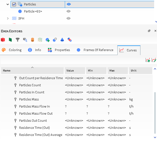
Table 5: Particle Curves options for Particle Instantaneous Energies
Function | Description |
|---|---|
Energy Delta | When the Particle Instantaneous Energies Module is enabled (see also About Particle Instantaneous Energies), this provides a variation (delta) in total energy of the particles recorded during an interval between two consecutive output time. Notes:
Tip: This Curve can be especially useful when computed in User Processes created on the Particles as it will represent the energy delta in only that subset of particles. |
(See also About Particles Energy Spectra and About Contacts Energy Spectra)
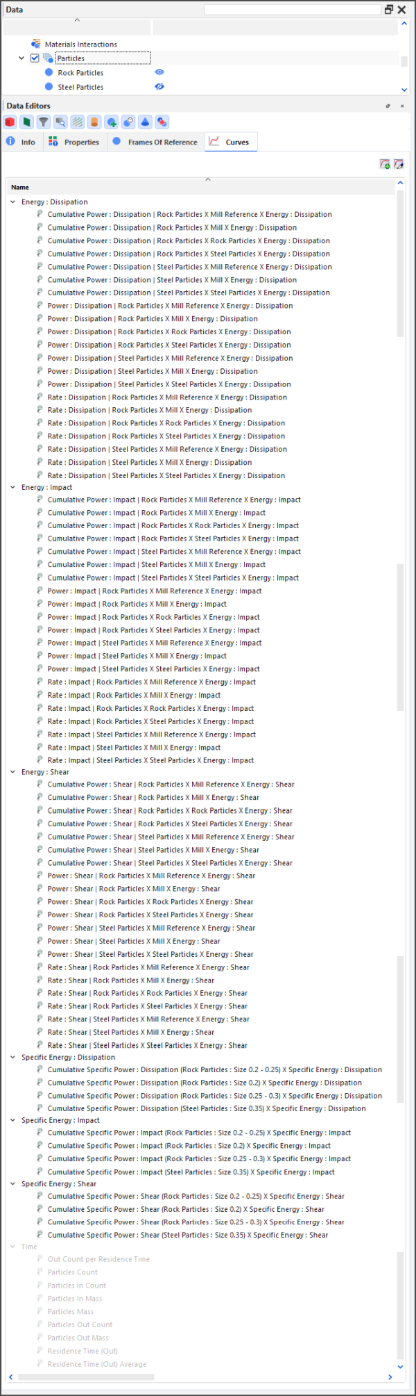
Table 6: Particle Curves options for Energy Spectra
Function | Description |
|---|---|
Energy Types | |
Energy : Dissipation (Specific Energy : Dissipation) | When the Particles Energy Spectra module and/or the Contacts Energy Spectra module is enabled (see also About Particles Energy Spectra and About Contacts Energy Spectra), and the Dissipation Energy checkbox on that module is enabled, this provides the dissipated energy component of the specified curve. |
Energy : Impact (Specific Energy : Impact) | When the Particles Energy Spectra module and/or the Contacts Energy Spectra module is enabled (see also About Particles Energy Spectra and About Contacts Energy Spectra), and the Impact Energy checkbox on that module is enabled, this provides the impact energy component of the specified curve. |
Energy : Shear (Specific Energy : Shear) | When the Particles Energy Spectra module and/or the Contacts Energy Spectra module is enabled (see also About Particles Energy Spectra and About Contacts Energy Spectra), and the Shear Energy checkbox on that module is enabled, this provides the shear energy component of the specified curve. |
Energy Curves | |
Cumulative Power | When the Contacts Energy Spectra module is enabled (see also About Contacts Energy Spectra), this provides for each energy type collected (Dissipation, Impact, and/or Shear) and contact pair (Particle-Particle or Particle-Geometry) indicated, the sum of all energy coming from a collision with energy greater than a specified energy level divided by the amount of time existing between the module's Start Time and the current output time. |
Power | When the Contacts Energy Spectra module is enabled (see also About Contacts Energy Spectra), this provides for each energy type collected (Dissipation, Impact, and/or Shear) and contact pair (Particle-Particle or Particle-Geometry) indicated, the time average of energy resulting from all collisions that occur between the module's Start Time and the current output time. |
Rate | When the Contacts Energy Spectra module is enabled (see also About Contacts Energy Spectra), this provides for each energy type collected (Dissipation, Impact, and/or Shear) and contact pair (Particle-Particle or Particle-Geometry) indicated, the mean frequency of collision throughout the module's Start Time and the current output time. |
Cumulative Specific Power | When the Particles Energy Spectra module is enabled (see also About Particles Energy Spectra), this provides for each Specific Energy type collected (Dissipation, Impact, and/or Shear) and Particle set - Particle Size group indicated, the sum of all specific energy coming from a collision with energy greater than a specified energy level divided by the amount of time existing between the module's Start Time and the current output time. |
(See also About Solver Parameters.)
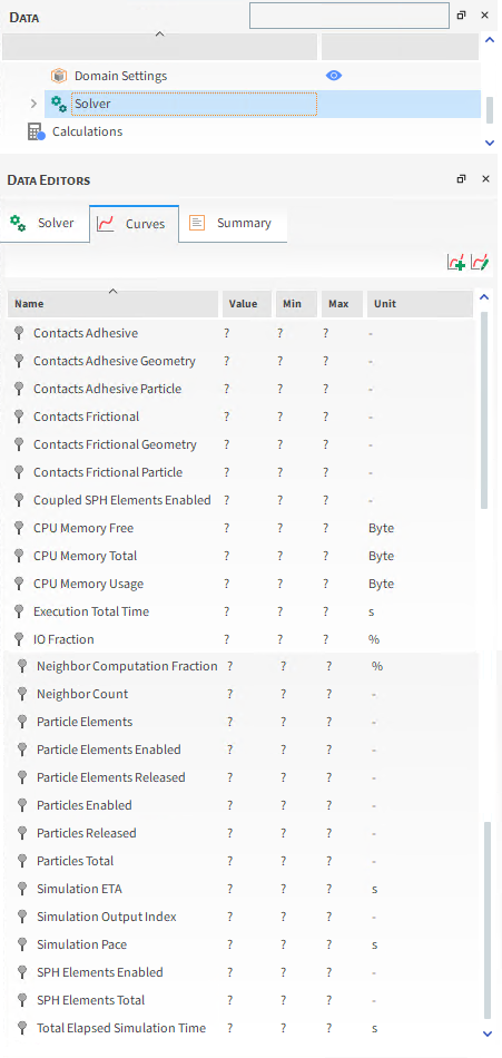
Table 7: Curves options for the Solver entity
Function | Description |
|---|---|
Contacts Adhesive | The total number of particle-to-particle and particle-to-boundary contacts resulting from adhesion that have been made. (For more information about Adhesive Forces, see About Physics Parameters). |
Contacts Adhesive Geometry | The total number of particle-to-boundary contacts resulting from adhesion that have been made. (For more information about Adhesive Forces, see About Physics Parameters). |
Contacts Adhesive Particle | The total number of particle-to-particle contacts resulting from adhesion that have been made. (For more information about Adhesive Forces, see About Physics Parameters). |
Contacts Frictional | The total number of particle-to-particle and particle-to-boundary contacts in which the entities are physically touching each other. |
Contacts Frictional Geometry | The total number of particle-to-boundary contacts in which the entities are physically touching each other. |
Contacts Frictional Particle | The total number of particle-to-particle contacts in which the entities are physically touching each other. |
CPU Memory Free | The amount of memory available on the CPU. |
CPU Memory Total | The total amount of memory—both used and unused—the CPU has. |
CPU Memory Usage | The amount of memory that is being used on the CPU. |
Enabled Coupled SPH Elements | The total amount of SPH elements figured inside the particles for the purpose of interacting with external SPH elements in an SPH-DEM interaction simulation. |
Enabled SPH Elements | The total number of SPH Elements that are currently located within the simulation boundaries. |
Execution Total Time | The amount of time (duration) that has passed since the simulation started processing again from a stopped state. |
GPU Count | The total number of GPU cards that are processing the simulation. |
GPU Memory Free | The amount of memory available on the GPU(s) that is processing the simulation. |
GPU Memory Total | The total amount of memory—both used and unused—that the GPU(s) processing the simulation has. |
GPU Memory Usage | The amount of memory being used on the GPU(s) processing the simulation. |
Halo Particles: Ratio | The ratio between the number of halo particles and the total number of particles in the domain. |
Halo SPH Elements | In multi-GPU runs, Halo SPH Elements are those that are located in the overlapping devices domain regions and therefore are present simultaneously in two GPU devices. For the Halo SPH Elements, both devices compute the collision forces but only one of the devices accumulates these data in order to perform velocity and displacement calculations. |
IO Fraction | The fraction of each unit of simulation time allotted to I/O (input/output), which involves writing to and reading from the simulation information on disk. This fraction is a value between 0.0 and 1.0: when closer to 0.0, less wall clock time was spent on I/O. |
Neighbor Computation Fraction | The fraction of each unit of simulation time allotted to the counting of neighbor particles, which in turn help identify possible collisions. This is a value between 0.0 and 1.0: when closer to 0.0, less wall clock time was spent searching for neighboring particles. |
Neighbor Count | The total amount of neighboring particles detected. This value indicates the number of possible collision events. |
Particles Elements | For particles composed of multiple elements (also known as meshed), this is the total number of individual elements that will be injected into the simulation during the entire Simulation Duration. |
Particle Elements Enabled | For particles composed of multiple elements (also known as meshed), this is the total number of individual elements that are currently located within the simulation boundaries. |
Particle Elements Released | For particles composed of multiple elements (also known as meshed), this is the total number of individual elements that have appeared in the simulation thus far. |
Particles Enabled | The total number of whole particles that are currently located within the simulation boundaries. This is useful for determining breakage efficiency. Note: Once a whole particle is broken into fragments, it is no longer counted towards this value. |
Particle Fragments | When Instantaneous Breakage parameters are set, this provides the total number of individual fragments the whole particles have been broken into. This is useful for determining breakage efficiency. |
Particles Released | The total amount of all whole particles that have appeared in the simulation. |
Particles Total | The total number of whole particles that will be injected into the simulation during the entire Simulation Duration. (See also About Solver Parameters). This includes particles that have yet to be released but does not include fragments resulting from Instantaneous Breakage. |
Simulation ETA | The estimated amount of time (duration) required to finish processing the simulation. This value considers the current simulation configuration. |
Simulation Output Index | The output file saved for the output time (See also Refer to the Rocky Title Bar for Simulation Progress Details). This is useful for determining at what point during the simulation an event of interest occurred. |
Simulation Pace | The estimated amount of time (duration) required to advance the simulation one second. This value considers the current simulation configuration. |
Halo SPH Elements Ratio | The ratio between the number of halo elements and the total number of SPH Elements in the domain. |
Total Elapsed Simulation Time | The total amount of time (duration) that the simulation has been processing since it was originally started. This is calculated by adding up the various Execution Total Times from multiple, separate executions (stops and resumes) of the simulation. |
(See also About Creating and Applying Motion Frames and I cannot find some Properties or Curves in this version of Rocky). Tip:See additional information in the About Curves for Imported Geometries and Motion Frames section above.
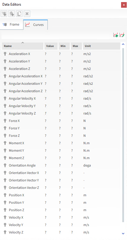
Table 8: Curves options for Motion Frames
Function | Description |
|---|---|
Acceleration X | The motion frame's acceleration along the X axis. |
Acceleration Y | The motion frame's acceleration along the Y axis. |
Acceleration Z | The motion frame's acceleration along the Z axis. |
Angular Acceleration X | The X-component of the motion frame's angular acceleration vector. |
Angular Acceleration Y | The Y-component of the motion frame's angular acceleration vector. |
Angular Acceleration Z | The Z-component of the motion frame's angular acceleration vector. |
Angular Velocity X | The X-component of the motion frame's angular velocity vector. |
Angular Velocity Y | The Y-component of the motion frame's angular velocity vector. |
Angular Velocity Z | The Z-component of the motion frame's angular velocity vector. |
Force X | The force applied to the motion frame along the X axis. |
Force Y | The force applied to the motion frame along the Y axis. |
Force Z | The force applied to the motion frame along the Z axis. |
Moment X | The moment (torque) applied to the motion frame along the X axis. |
Moment Y | The moment (torque) applied to the motion frame along the Y axis. |
Moment Z | The moment (torque) applied to the motion frame along the Z axis. |
Orientation Angle | For the set of axes that represents the Motion Frame's orientation, this is the rotation angle about the defined Relative Rotation Vector. See also About Creating and Applying Motion Frames to Custom Geometries. |
Orientation Vector X | The X-component defining the vector about which the motion frame axes is rotated. See also About Creating and Applying Motion Frames to Custom Geometries. |
Orientation Vector Y | The Y-component defining the vector about which the motion frame axes is rotated. See also About Creating and Applying Motion Frames to Custom Geometries. |
Orientation Vector Z | The Z-component defining the vector about which the motion frame axes is rotated. See also About Creating and Applying Motion Frames to Custom Geometries. |
Position X | The coordinate location of the motion frame axes' center point as specified in the X direction. |
Position Y | The coordinate location of the motion frame axes' center point as specified in the Y direction. |
Position Z | The coordinate location of the motion frame axes' center point as specified in the Z direction. |
Velocity X | The translational velocity of the motion frame as defined in the X direction. |
Velocity Y | The translational velocity of the motion frame as defined in the Y direction. |
Velocity Z | The translational velocity of the motion frame as defined in the Z direction. |
What would you like to do?
See Also:
There are many default properties provided on the Properties and Curves tabs for a simulation entity (Particles, 1-Way LBM, 1-Way Fluent, Solver, individual geometry components, individual Motion Frames, Eulerian Statistics, and any individual User Processes linked to these entities) but you can also create and edit custom properties to create your own unique data sets.
Note: Though customizing Properties also applies to Eulerian Statistics, because Eulerian Statistics is a unique User Process based only upon the Particles entity, you can also add new Particles Properties to a Eulerian Statistics User Process. See About Customizing Eulerian Statistics Properties for more information.
Customizing Properties is accomplished from the upper-right corner of the Properties tab. Customizing Curves is accomplished from the upper-right corner of the Curves tab.
Tip: To see walk-through examples of customizing a property or curve, refer to the following Tutorials:
See the images and tables below to help you understand how to add and edit your own unique properties or curves.
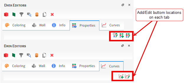
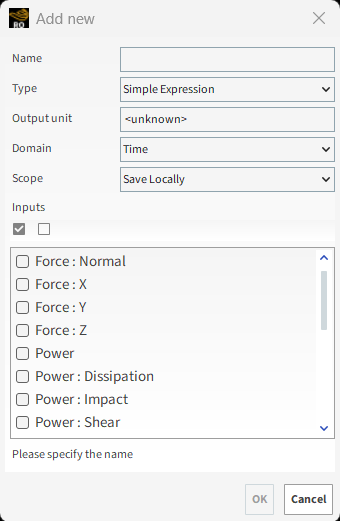
Table 1 : Add new dialog options (property or curve)
Setting | Description | Range |
|---|---|---|
Name | Enables you to specify a unique identifier for the property or curve. | 99 character limit |
Type | Specifies how the expression will be defined.
Note: The expression is entered on the Custom Property or Custom Curves dialog that appears after you click OK. (See below section.) | Simple Expression; Advanced Expression (script) |
Output unit | The units you want assigned to the property or curve. | <unknown> (see also Recognize Data Placeholders); any applicable unit defined in Rocky (see also About Setting Your Unit System). |
Inputs | Lists all existing properties or curves available for the entity, including any custom properties or curves you have defined. | Automatically provided. (See also Use Properties and Curves). |
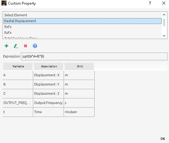
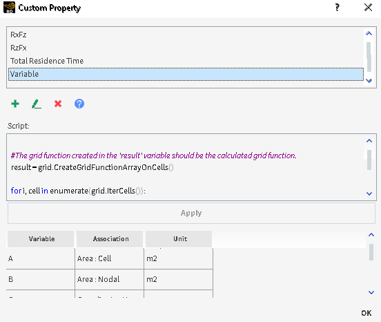
Table 2: Custom dialog options (properties and curves)
Setting | Description | Range |
|---|---|---|
Expression | When the Type of the custom property or curve is Simple Expression, this is where you define the mathematical expression for the property or curve. Note: The expression in Rocky follows the syntax of the Python NumPy library. | |
Script | When the Type of the custom property or curve is Advanced Expression (script), this is where you use Python code to define the details of the property or curve. Note: The code you enter here is not the same as a Rocky script which has a different structure and purpose. | |
Variable | Column that lists the variable names available for you to use within the expression or script. Specifically:
The following variables are also in the product but are not recommended for use at this time:
| Automatically provided |
Association | Column that maps the Variable name to its Rocky property. | Automatically provided |
Unit | Column that lists the unit used by the Variable. | Automatically provided |
What would you like to do?
See Also:
You can customize Eulerian Statistics Properties just like any other Property. (See also About Customizing Properties or Curves.) However, unlike other Properties, you may also add new Particles Properties to your default list of Eulerian Statistics Properties.
Eulerian Statistics is a unique User Process based only upon the Particles entity (see also About Eulerian Statistics). The primary purpose is to analyze specific locations in a simulation, and not necessarily the individual particles that are in them. For example, you might use Eulerian Statistics to analyze the average particle mass inside each individual block to see at a glance which region of your simulation has a higher density of particles. So while the analysis uses information about the particles, it is really the individual blocks and the simulation locations they represent that are the primary focus.
Thus, unlike other User Processes, which offer default Properties shared by the simulation entity upon which they were created, Eulerian Statistics has its own set of unique Properties. (See also About Properties.) To these default functions, you can add additional Properties from the Particle entity upon which the Eulerian Statistics User Process is based.
See the images and table below to understand how to add Particle Properties to your Eulerian Statistics User Process.
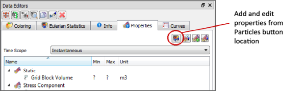
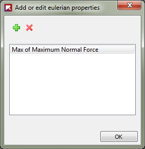
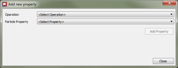
Table 1 : Add new property dialog options
Setting | Description | Range |
|---|---|---|
Operation | The operation that will be applied to the Particle Property(s) selected. Specifically:
| Average; Min; Max; Sum; Volume Fraction Average; Weighted Average; Standard Deviation |
Particle Property | Lists all existing properties available for the Particles entity, including any custom properties you have defined. | Automatically provided. (See also About Properties.) |
Weight Property | When Weighted Average is chosen from the Operation list, this lists all existing properties available for the Particles entity, including any custom properties you have defined. | Automatically provided. (See also About Properties.) |


What would you like to do?`
See Also:
You can customize the SPH Eulerian Solution Properties just like any other Property. (See also About Customizing Properties or Curves.)
Eulerian Solution allows you to analyze specific locations in a simulation where there are no SPH elements in a specific time step. For example, you might use Eulerian Solution to analyze the average density of each individual cell see at a glance which region of your simulation has a higher fluid density. So while the analysis uses information about the SPH elements, it is really the individual cells and the simulation locations they represent that are the primary focus.
The Eulerian Solution option has its own set of unique Properties. (See also About Properties.) To these default functions, you can add additional Custom Properties.
See the image and table below to understand what Properties are available when using the Eulerian Solution.
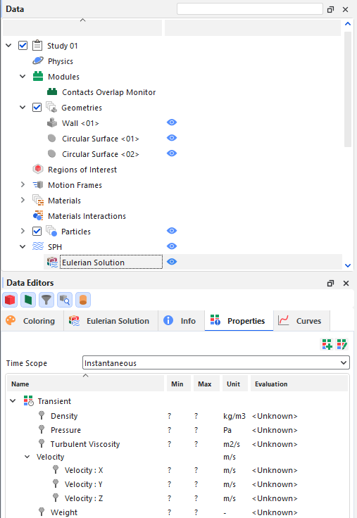
Table 1 : Properties available in the SPH Eulerian Solution
Property Name | Description |
|---|---|
Density | The average density of each Eulerian Solution cell |
Pressure | The average pressure of each Eulerian Solution cell |
Turbulent Viscosity (only available if a turbulence model is enabled) | The average turbulent viscosity of each Eulerian Solution cell |
Velocity: X | The average X direction velocity of each Eulerian Solution cell |
Velocity: Y | The average Y direction velocity of each Eulerian Solution cell |
Velocity: Z | The average Z direction velocity of each Eulerian Solution cell |
Weight | Property that indicates from 0 to 1 how much fluid is present in a cell (0 no fluid, 1 full of fluid) |
See Also:
A Time Statistics Property enables you to limit a Property by a particular time range and operation that you specify. That new property definition becomes its own unique Property, which you can then use just like any other Property for further analysis. This method is useful when you need to focus your analysis upon only the average (max, min, or sum) values for a Property calculated during a certain time period of your simulation—after steady state has been reached or once particles start leaving the simulation boundaries, for example.
Tip: To see a walk-through example of adding and using a Particle Time Statistics Property, review Tutorial - Tablet Coater in the Rocky Tutorial Guide.
Time statistics are available for all Properties (see also About Properties) except those accessible via the main Particles, the 1-Way Fluent CFD Coupling method, and Contacts entities. This includes support for all of the following entities:
Individual Particle set Properties. (See also About Intra-Particle Collision Statistics.)
Eulerian Statistics User Process Properties. (See also About Eulerian Statistics.)
Individual Geometry component Properties.
1-Way LBM Properties. (See also About Using the 1-Way LBM Method.)
Once you add a Time Statistics Property for one of the above supported entities, it will be available for all entities of the same type.
With regular Properties, the results by default only take into account data calculated for the current timestep (Figure 5.36: The same mill and timestep as above, but showing one Property (standard Property)). By using by Eulerian Statistics User Process, for example, and then customizing the Properties (see also About Customizing Eulerian Statistics Properties), you could also show an operation (average, for example) for that same Property within the individual Eulerian blocks, but still for only one timestep at a time (Figure 5.37: The same mill and timestep as Figure 2 but with Eulerian Statistics applied showing the average values of a Property within each Eulerian block (custom Property)). With Time Statistics Properties, you can now apply an operation over a specific time range (Figure 5.38: The same mill and Eulerian Statistics applied as above, but now those values are averaged over a set range of time (Time Statistics Property)).
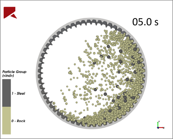
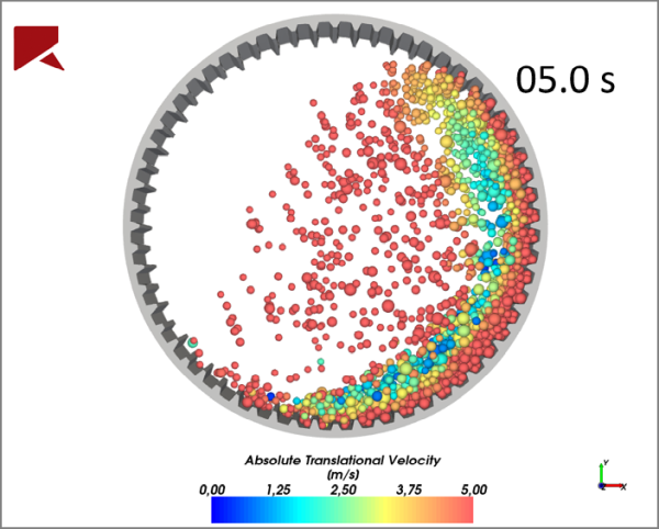
Figure 5.37: The same mill and timestep as Figure 2 but with Eulerian Statistics applied showing the average values of a Property within each Eulerian block (custom Property)
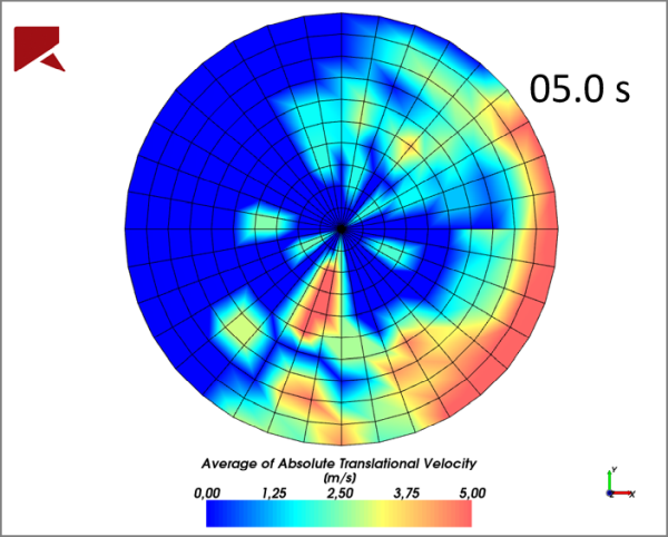
Figure 5.38: The same mill and Eulerian Statistics applied as above, but now those values are averaged over a set range of time (Time Statistics Property)
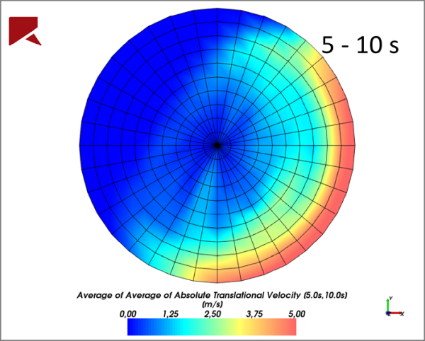
Tip: For more information about using Time Statistics for Eulerian Statistics, see the following article: Time Statistics For Eulerian Statistics And Smoothed Plots
Like Customizing a Property (see About Customizing Properties or Curves), adding and editing Time Statistics Properties is accomplished from the upper-right corner of the Properties tab. See the images and tables below to help you understand how to add and edit Time Statistics Properties.
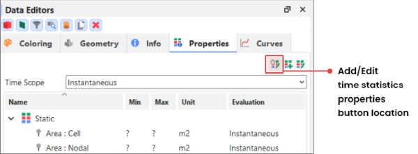

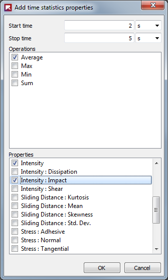
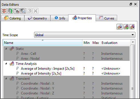
Table 1: Edit time statistics property dialog options
Setting | Description | Range |
|---|---|---|
Start Time | The amount of time into your simulation that you want calculations to start being included in the operation selected for the Time Statistics Property. Note: Neither Time values are editable until you add a Time Statistics Property. To accomplish this, click the Add button. (See also Add a Time Statistics Property.) | Positive values |
Stop Time | The amount of time into your simulation that you want calculations to stop being included in the operation selected for the Time Statistics Property. Tip: If you want your range to extend to the end of your simulation, enter a very large number, such as 1000. Note: Neither Time values are editable until you add a Time Statistics Property. To accomplish this, click the Add button. (See also Add a Time Statistics Property.) | Positive values |
Table 2: Add time statistics property dialog options
Setting | Description | Range |
|---|---|---|
Start Time | The amount of time into your simulation that you want calculations to start being included in the operation selected for the Time Statistics Property. Between this and the Stop Time value defines the time range for the new Time Statistics Property. | Positive values |
Stop Time | The amount of time into your simulation that you want calculations to stop being included in the operation selected for the Time Statistics Property. Between the Start Time and this value defines the time range for the new Time Statistics Property. Tip: If you want your range to extend to the end of your simulation, enter a very large number, such as 1000. | Positive values |
Operations | Enables you to choose one or more operations to apply to the Property data within the time range you selected. One unique Time Statistics Property will be created per Operation and Property selected. Specifically:
| Average; Min; Max; Sum |
Property | Enables you to choose one or more Properties to which you can apply the selected Operations over the time range you selected. One unique Time Statistics Property with the selected time range will be created per Property and Operation selected. | List provided automatically |


What would you like to do?`
See Also:
The concept of particle upscaling refers to the way Rocky treats post-processing data and statistics from individual elements of a Multiple Element (meshed) particle. While the Rocky solver always computes multi-element properties per individual element, upscaling determines whether or not the application extends those individual properties to the whole particle itself.
In general, if a meshed particle is upscaled, which is the default setting (as shown below on the left), post-processing results will be provided for the whole particle. If a meshed particle is not upscaled, meaning the setting was disabled (as shown below on theright) post-processing results will be provided for each individual Element making up the particle.
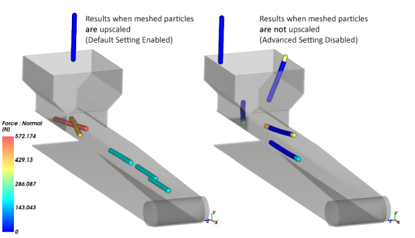
How this is applied in your simulation is determined by the Meshed Particles Upscaling checkbox in the Study parameter on the Data Editors (as shown below). (See also About Setting Global Preferences.)
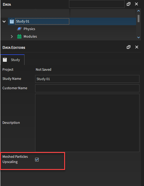
Note: As this setting applies only to post-processing analyses, you can adjust this parameter at any time during your simulation. However, you will need to close and reopen your Rocky project for you to see the change applied to your results.
By default, the Meshed Particles Upscaling checkbox is enabled. In these cases, any Multi-Element particle used in the simulation is an upscaled one and most post-processing properties and curves will be provided for the particle as a whole (Figure 5.43: Example results when meshed particle upscaling is enabled (left) and disabled (right), left).
There are some known exceptions to this rule, however. These include the Particles and Particle set properties and curves listed in the tables below. In these cases, even when the simulation has meshed particles set to be upscaled, the post-processing data might still be provided for the individual Elements (upscaling is ignored — Tables 1 and 2) or will not be provided at all (not listed in Properties tab — Table 3).
Table 1: Upscaling exceptions for Particle Set Properties (Per Set Only)
Effects of upscaling are ignored for this Property | How Collected | See Also |
|---|---|---|
(All Intra-particle properties) | Intra-particle Collision Statistics |
Table 2: Upscaling exceptions for Particle Curves (Simulation Wide)
Effects of upscaling are ignored for this Curve | How Collected | See Also |
|---|---|---|
(All Inter-group curves) | Inter-group Collision Statistics |
Table 3: Upscaling exceptions for Particles Properties (Simulation Wide)
Upscaling results in this Property not being listed on the Properties tab | How Collected | See Also |
|---|---|---|
Duration | Inter-particle Collision Statistics | |
Velocity : Impact | Inter-particle Collision Statistics | |
Moment of Inertia | Automatic | |
Orientation Angle | Automatic | |
Orientation Vector X | Automatic | |
Orientation Vector Y | Automatic | |
Orientation Vector Z | Automatic | |
Particle Equivalent Diameter | Automatic | |
Particle Size | Automatic |
If you decide to clear the Meshed Particles Upscaling checkbox (Figure 5.44: Meshed Particles Upscaling, Study parameter), any Multi-Element particle used in the simulation will have its properties or curves provided per individual Element (Figure 5.43: Example results when meshed particle upscaling is enabled (left) and disabled (right), right).
Notes:
Because the properties and curves listed above in Tables 1 and 2 are ignoring the effects of upscaling, disabling upscaling in these cases results in the same outcome as if it was enabled: for Multi-Element particles, the properties and curves are provided per individual Element only.
In this version of Rocky, disabling upscaling is the only way to obtain the properties shown above in Table 3.
See Also:
Note: This particular process does not apply to any Particles Properties added to a Eulerian Statistics User Process. See About Customizing Eulerian Statistics Properties for more information.
From the Data panel, select the entity containing the property you want to change or remove. This can include a conveyor or imported geometry component, Particles, 1-Way LBM, Solver, or individual Motion Frame.
From the Data Editors panel, select either the Properties or Curves tab containing the custom property you want to change or remove.
From the upper right corner of the tab, click the Edit custom… button.
From the Custom… dialog, select the name of the property you want under Select Element.
Do any or all of the following:
To change the Name, Output unit, or Inputs used by the property, click the Edit…. button.
To change the expression listed in either the Expression or Script boxes, make your changes directly within the dialog.
To remove the function, click the Remove custom… button.
Click OK.
See Also:
Note: This particular process does not apply to any Particles Properties added to a Eulerian Statistics User Process. See About Customizing Eulerian Statistics Properties for more information.
From the Data panel, select the entity to which you want to add a custom property. This can include a conveyor or imported geometry component, Particles, 1-Way LBM, 1-Way Fluent, Solver, individual Motion Frame, or any individual User Process linked to these entities.
From the Data Editors panel, select one of the following:
The Properties tab, to create a custom function applying to each individual element in a structure (e.g., particle, geometry triangle, or air flow node).
The Curves tab, to create a custom property applying to the entire entity as a whole.
From the upper right corner of the tab, click the Add new custom… button.
From the Add new dialog, enter the information you want, and then click OK. Tips: To select all inputs, click the Check All button. To clear all inputs, click the Uncheck All button.
From the Custom… dialog, define your expression in either the Expression or Script box shown using the variables provided in the dialog's table.
Click OK. The new custom property appears in the functions list sorted by Name. (See also Name Components to Affect Sort Order.)
See Also:
From the Data panel, under User Processes, select the Eulerian Statistics User Process you want. (See also Divide a Cube or Cylinder User Process into Many Analysis Blocks.)
From the Data Editors panel, select the Properties tab.
From the upper-right corner of the tab, click the Add and edit properties from particles button.
From the Add or edit eulerian properties dialog, click the Add button.
From the Add new property dialog, select the options you want, and then click Add Property. The new function appears on the Properties tab.
Repeat step 5 for each new function you want to add.
Click Close. The function(s) you added appear in the Add or edit eulerian properties dialog.
Click OK.
See Also:
Note: This procedure applies only to Particle Properties that you have added to a Eulerian Statistics User Process. (See also Add a Particle Property to a Eulerian Statistics User Process.) You may not remove the Particle Properties provided by default with Rocky.
From the Data panel, under User Processes, select the Eulerian Statistics User Process containing the Particle Property you want to remove.
From the Data Editors panel, select the Properties tab.
From the upper-right corner of the tab, click the Add and edit properties from particles button.
From the Add or edit eulerian properties dialog, select the Particles Property you want from the list, and then click the Remove button.
Click OK to close the dialog. Your changes are reflected in the Properties list for the Eulerian Statistic User Process.
See Also:
Note: This particular process does not apply to the main Particles or 1-Way Fluent entities, nor any User Process created from the Particles entity, with the exception of Eulerian Statistics. (See also About Eulerian Statistics.)
From the Data panel, select the entity to which you want to add a Time Statistics Property. This can include any individual geometry component, individual Particle set, 1-Way LBM, Eulerian Statistics User Process, or any other User Process created from a non-Particles entity.
From the Data Editors panel, select the Properties tab.
From the upper right corner of the tab, click the Add and edit time statistics properties button.
From the Edit time statistics properties dialog, click the Add button.
From the Add time statistics properties dialog, do all of the following:
Enter the time range you want to focus upon in the Start time and Stop time boxes.
From the Operations list, select one or more operations you want to apply to the selected Property across the time range selected.
From the Properties list, select one or more Properties.
Click OK. One unique Time Statistics Property per Property and Operations combination appears in the Edit time statistics properties dialog.
Click OK. For all entities of the same type you initially selected, the new Property(s) appear on the Properties tab of the Data Editors panel under Time Analysis.
See Also:
Note: This particular process does not apply to the main Particles, 1-Way Fluent, nor Contacts entities, nor any User Process created from the Particles entity, with the exception of Eulerian Statistics. (See also About Eulerian Statistics.)
From the Data panel, select the entity for which you want to edit a Time Statistics Property that you have already added. (See also Add a Time Statistics Property.) This can include any individual geometry component, individual Particle set, 1-Way LBM, Eulerian Statistics User Process, or any other User Process created from a non-Particles entity.
From the Data Editors panel, select the Properties tab.
From the upper right corner of the tab, click the Edit time statistics properties button.
From the Edit time statistics properties dialog, select the Time Statistics Property you want to edit or remove from the list, and then do one of the following:
To edit it, change the Start time or Stop time values.
To remove it, click the Remove button. Your changes are reflected in the dialog.
Click OK to close the dialog. Your changes are reflected in the Properties list under Time Analysis.
See Also: