


Rocky comes integrated with several Ansys products including Mechanical, Fluent, Motion, Minerva, and optiSLang.
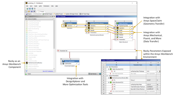
Rocky can also integrate with Ansys Workbench. Working through Workbench enables Rocky to couple its abilities with other Ansys products - including Mechanical, Fluent, DesignXplorer, and SpaceClaim - which enables you to define design points for parametric cases, and solve more kinds of solutions in more complex and innovative ways.
When a Rocky project is connected to Ansys Mechanical though Workbench, an External Coupling component becomes enabled in the Rocky Data panel. This component enables you to define the kind of data gets shared between the programs, such as the geometry loads.
This section covers the following topics:
Ansys Workbench is a product you can use to more easily connect, share, automate, and keep organized data across various programs. When used with Rocky, Workbench can help you accomplish many time-saving tasks like the ones described in the sections below.
Tip: To learn which versions of Ansys-including Workbench, SpaceClaim, Mechanical, Fluid, and other products-are compatible with this version of Rocky, refer to System Requirements.
This section covers the following topics:
ROCKY INTEGRATION IN WORKBENCH
WORKBENCH INTEGRATION IN ROCKY
MAXIMIZE THE DESIGN OF YOUR GEOMETRY COMPONENTS BY USING ANSYS SPACECLAIM
PARAMETERIZE SIMULATION AND SETUP COMPONENTS BY USING ANSYS DESIGNXPLORER
CONDUCT FEA ANALYSIS OF PARTICLE FORCES ACTING UPON GEOMETRY COMPONENTS BY USING ANSYS MECHANICAL
STUDY HOW CFD FLUID AND THERMAL PROPERTIES AFFECT PARTICLE FLOW BY USING ANSYS FLUENT
1-WAY AND 2-WAY COUPLING WITH FLUENT IN WORKBENCH
1-WAY ANSYS FLUENT COUPLING WITH WORKBENCH
UNRESOLVED 2-WAY ANSYS FLUENT COUPLING WITH WORKBENCH
SEMI-RESOLVED 2-WAY ANSYS FLUENT COUPLING WITH WORKBENCH
ROCKY INTEGRATION IN WORKBENCH
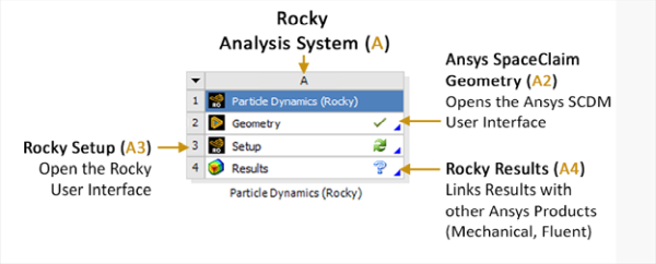
Once you open Workbench and create a new Project, you can from the Toolbox panel, expand the Analysis Systems item, and then drag and drop Particle Dynamics (Rocky) to the Project Schematic (Figure 8). Note: This item will be referred to as the "Rocky" block for simplicity.
This creates a link between your Workbench project and the Rocky program. From here, you can either start a new Rocky project from within Workbench (Edit), or import a Rocky project into Workbench that you have already set up (Import Setup).
The link between your Workbench project and your Rocky project means that data will be automatically transferred between the two programs. In addition, it exposes Rocky input and output parameters, so you can explore Workbench capabilities such as evaluating multiple design points, creating Rocky cases automatically, and then running them through the weekend. (See also About Defining and Using Input Variables and About Defining Output Variables.)
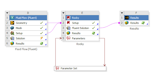
The new Rocky Analysis System block (A) is made up of the components described in Figure 9.
By interacting with the Rocky Analysis System block, and linking other items from the Workbench Analysis System-such as the Transient Structural block or the Static Structural block-to the Rocky items listed, you can have Workbench perform many different tasks in Rocky. This includes one-way coupled approaches with Ansys Mechanical, one-way coupled approaches with Ansys Fluent, standalone parametric studies, and more.
Note: In this version of Rocky, projects coupled with Ansys Workbench now use Ansys Discovery as default for Geometry imports and conversions. Therefore, if Ansys Discovery is not installed, you will get an error message when trying to convert geometries into .STL in Rocky-Workbench coupled projects.
WORKBENCH INTEGRATION IN ROCKY
If you have linked to Rocky from within Workbench, an External Coupling entry will appear in the Rocky Data panel (Figure 10).
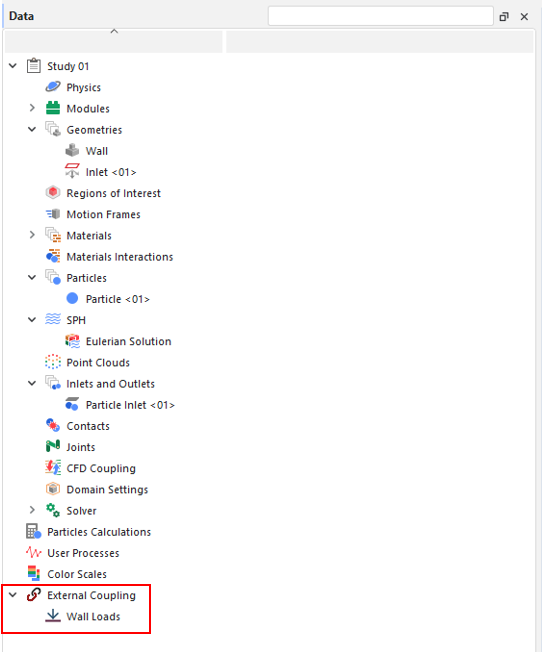
For Rocky projects opened through Workbench that are not coupled with Ansys Mechanical, this component will still appear in the Data panel but can be ignored.
WORKBENCH INTEGRATION RESOURCES
To learn more about Workbench integration with Rocky, and to see Workbench in action, refer to the following resources:
See Also:
MAXIMIZE THE DESIGN OF YOUR GEOMETRY COMPONENTS BY USING ANSYS SPACECLAIM
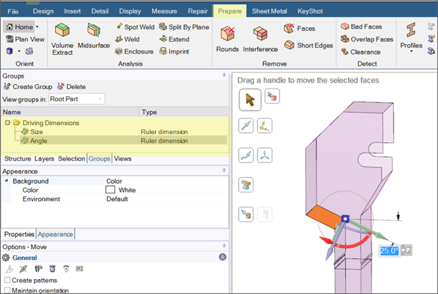
This is accomplished through Workbench by connecting your Rocky project with Ansys SpaceClaim 3D geometry files, thereby enabling you to change equipment components in SpaceClaim (Figure 1) and have those geometry changes be automatically updated in your Rocky project.
Note: In this version of Rocky, projects coupled with Ansys Workbench now use Ansys Discovery as default for Geometry imports and conversions. Therefore, if Ansys Discovery is not installed, you will get an error message when trying to convert geometries into .STL in Rocky-Workbench coupled projects.
Tip: To see walk-through examples of modifying your geometries in SpaceClaim for use in your Workbench-connected Rocky projects, refer to the following Tutorials:
PARAMETERIZE SIMULATION AND SETUP COMPONENTS BY USING ANSYS DESIGNXPLORER
This is accomplished through Workbench by connecting your Rocky project with Ansys DesignXplorer, which enables you to set design goals and get immediate feedback on proposed changes. DesignXplorer includes correlation, design of experiments, response surface creation and analysis, optimization and six sigma analysis. In addition, integration with other Ansys products like SpaceClaim ensures that any geometry changes made are automatically updated in your Rocky project.
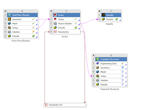
An example of such a project is shown in Figure 2 where varied geometrical inputs as well as Rocky inputs are used to evaluate the impact of those changes in Rocky output parameters. (See also About Defining and Using Input Variables and About Defining Output Variables.)
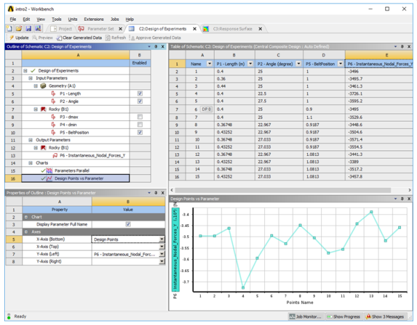
Using DesignXplorer through Workbench can be especially helpful when testing how small changes in geometry angles, sizes, or placements affects your material flow.
CONDUCT FEA ANALYSIS OF PARTICLE FORCES ACTING UPON GEOMETRY COMPONENTS BY USING ANSYS MECHANICAL
By using Workbench to connect your Rocky project with Ansys Mechanical, you can have Mechanical predict the stress and strain response of your geometry components when they are subjected to the granular loads that are calculated in Rocky.
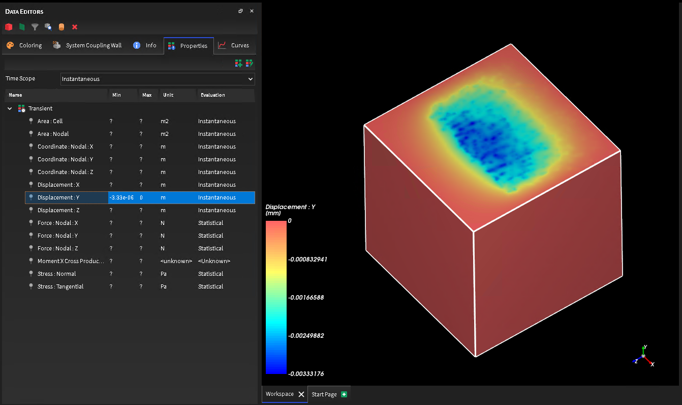
Workbench does this by first having Rocky calculate the particle forces and pressures on the geometry component. Next, it automatically exports that data from Rocky to Mechanical through Workbench, where Mechanical then uses those forces and pressures to perform static (at a single time - Figure 3) or transient (over a time range - Figure 4) structural analysis on the component.
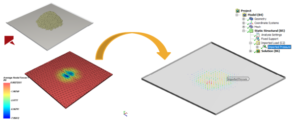
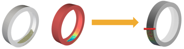
This approach is useful for analyzing the stress effects of particles upon a vibrating screen, for example, or for visualizing the mechanical deformation of a bucket excavator due to particle loads.
Tip: To learn more about using Mechanical to conduct Static and Transient FEA analyses in your Workbench-connected Rocky projects, refer to the following resources:
STUDY HOW CFD FLUID AND THERMAL PROPERTIES AFFECT PARTICLE FLOW BY USING ANSYS FLUENT
By using Workbench to couple your Rocky project 1-Way with Ansys Fluent, Rocky can calculate how the CFD fluid flow and heat transfer affects the DEM particle flow and related thermal properties (Figure 5).
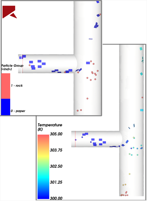
This approach is useful for studying how air flow affects various kinds of material flowing through a pipe, for example.
Tip: To see a walk-through example of a 1-Way coupled simulation with Ansys Fluent, refer to the following Tutorial: Tutorial 13 - DEM-CFD One Way Coupling With Ansys Fluent (Workbench).
1-WAY AND 2-WAY COUPLING WITH FLUENT IN WORKBENCH
From Rocky 23R1 it's possible to use both 1-way and 2-way CFD-DEM coupling analyses through Ansys Workbench. This functionality brings many advantages, such as:
Multiphysics Analyses Integration: With a single interface, it's possible to integrate multiple analyses, making it easy to see in the workflow project who is sending data to whom.
Automated Data Management: Save time without the need to manually transfer the results from one application to another.
Run multiple designs: to explore different scenarios.
Optimizing Exploration: parametric modeling capabilities in conjunction with optimization techniques to allow you to efficiently investigate the effects of input parameters on selected output parameters.
Workflow: all the necessary files are archived together, making it easy to share the project with other users.
To couple Rocky and Fluent in Workbench, follow the steps below:
1-WAY ANSYS FLUENT COUPLING WITH WORKBENCH
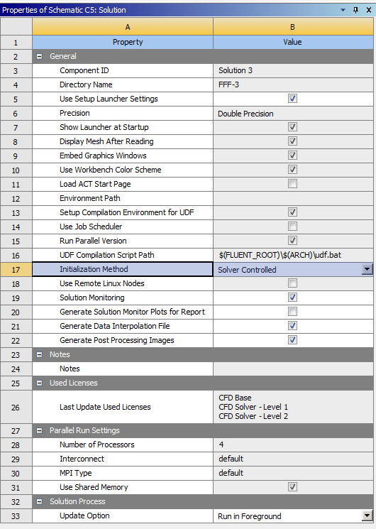
The 1-way coupling can use either a steady or transient flow field. For the 1-way coupling, select Fluent Solution Properties and change the Initialization Method to Solver Controlled;
Figure 2.52: For 1-way coupled simulations, the Initialization Method should be set as "Solver Controlled" in the Fluid Flow Solution Properties.
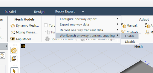
For a 1-way transient coupling, the option to Export the transient data must be enabled in the Rocky Export entry in Fluent.
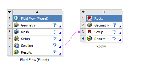
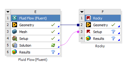
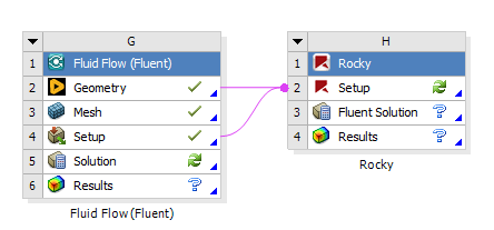
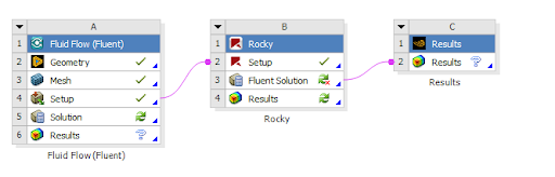
To use the flow field in the 1-way coupled simulation, link the Fluent Solution to the Rocky Setup.
For sharing the geometry between projects, link the Geometry of the Fluid project to the Geometry of the Rocky project. Doing so, the geometry will be automatically imported into Rocky.
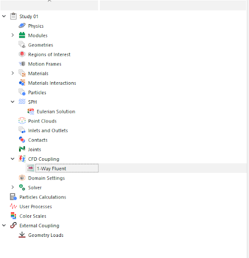
After the CFD solution is ready, when opening Rocky, the CFD Coupling entry in the Data Tree has the 1-Way Fluent mode selected.
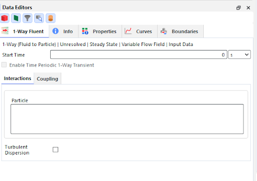
Open the 1-Way Fluent Data Editor and edit the coupling settings as usual.
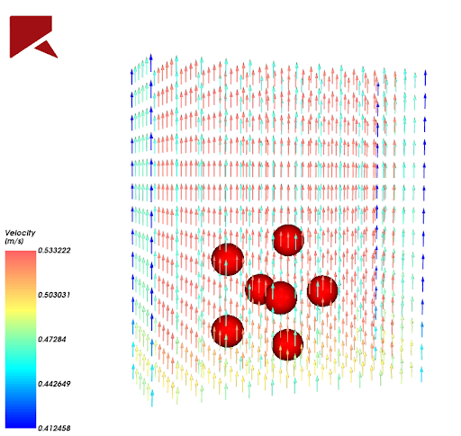
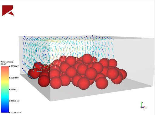
After run the simulation, the CFD and DEM results of the unresolved 1-way coupling can be simultaneously post-processed in Rocky Fluid. Quantities such as pressure and velocities can be analyzed and shown in the 3D view together with the particles.
Figure 2.58: The coloring tab of the 1-Way Fluent Data Editor allows the selection of which fluid information should be showed in the 3D view.
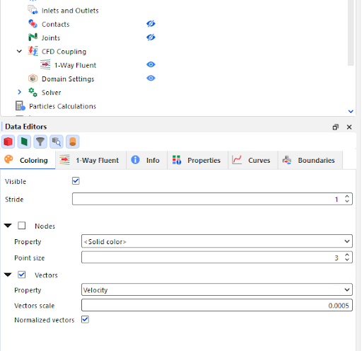
Figure 2.59: Vectors colored by the magnitude of the fluid velocity give insight to the flow field in 1-way coupled simulations.
UNRESOLVED 2-WAY ANSYS FLUENT COUPLING WITH WORKBENCH
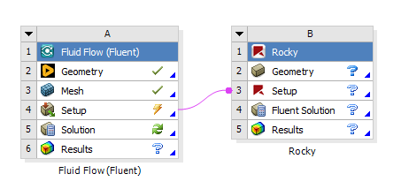
Drag the Fluent analysis onto the Project Schematic and set up the Fluent Project.
Important: You can only set up the 2-way coupled project if the Fluent Project is set up. Rocky looks for the .cas file for importing the necessary files for the 2-way coupling.
Drag a Rocky Analysis to the Project Schematics. Do not drop it on top of the Fluent setup.
Important: Do not drop it on top of the Fluent setup. The link must be created manually after both the two systems are placed at the Project Schematic.
Drag the Fluent Setup onto the Rocky Setup.
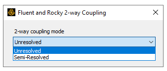
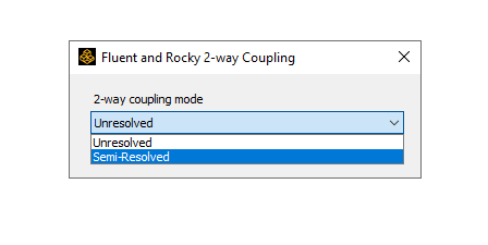
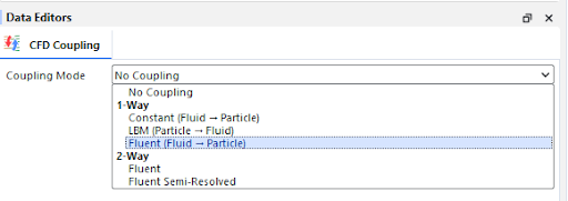
Select Unresolved as the 2-way coupling mode.
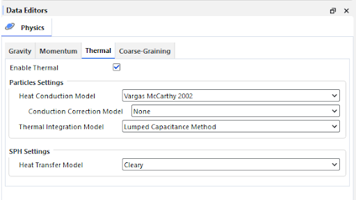
If the Fluent setup has Energy Model on, enable the Thermal in the Momentum tab of the Physics Data Editor in Rocky.`
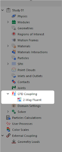
When opening Rocky, the CFD Coupling entry at the Data Tree has the 2-Way Fluent mode selected.
Open the 2-Way Fluent data panel and edit the coupling setup as usual.
Figure 2.65: The Unresolved 2-way coupling mode is enabled, and the coupling setting can usually be edited.

Set up the Fluent execution setting - select to run either in serial or parallel and the number of CPU processes that are used to solve CFD equations.
Important: As the Fluent run is controlled by Rocky in the 2-way coupling, the execution settings defined in the Rocky setup are used.
Figure 2.66: The Fluent tab allows the definition of the execution mode and the data used as the initial fluid field.
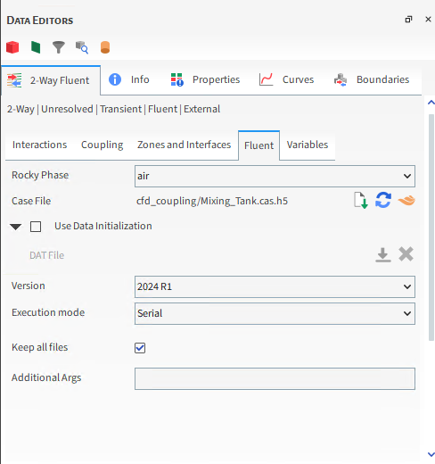
For prescribing an initial fluid field for the CFD solution, the .dat file should be imported at the Rocky setup.
Important: The current version does not allow the initial flow field to be imported from another Fluent run within the workbench. The fluent data file must be imported using the Fluent tab in Rocky.
For sharing the geometry between projects, link the Geometry of the Fluid project to the Setup of the Rocky project. Doing so, the geometry will be automatically imported into Rocky.
The CFD and DEM results of the unresolved 2-way coupling can be simultaneously post-processed in Rocky by opening the Setup entry of the Rocky project. Fluid quantities such as pressure and velocities can be analyzed and shown in the 3D view together with the particles.
The post-processing of additional fluid data can be done inside Fluent. For this purpose, a new Results component should be linked to the Fluent Solution of the coupled Rocky project.
Figure 2.69: The Fluent Solution entry should be used to send the fluid data for external post-processing.
The Fluent Solution entry in the Rocky project should be used for sending the fluid data to another software, such as a post-processing software or a structural analysis.
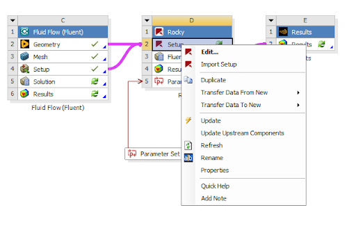
For updating changes made to an upstream step, such as changes in a Fluent boundary condition or CFD mesh, select Refresh from the Rocky Setup entry.
Important: Any change in the Fluent Setup should be made in the Fluent Project that is linked to the Rocky simulation, not from the 2-way Fluent Data Editor in the Rocky UI. The reason is that the CFD setup from the Fluid Flow project will be copied and used as the base setup for the coupled simulation. Any changes made using Rocky will be overwritten when updating the workbench project.
Figure 2.71: If something is changed in an upstream component, the Refresh option in the Setup entry should be used to update the Fluent project used in the coupled simulation.
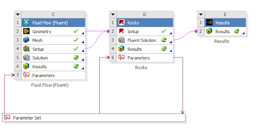
Inputs and Outputs parameters of the DEM simulation are exposed in the workbench as any other Ansys solver and can be used to evaluate several design points automatically.
Figure 2.72: The Fluent solution entry should be used for sharing the fluid data with another software, such as for structural analysis.

SEMI-RESOLVED 2-WAY ANSYS FLUENT COUPLING WITH WORKBENCH
Drag the Fluent analysis and set up the Fluent Project.
Drag a Rocky Analysis to the Project Schematics. Do not drop it on top of the Fluent setup.
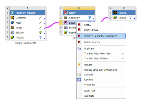
If the DEM simulation has no walls, you can Remove the Geometry Component.
Select Setup in the Rocky Project and click Edit. Select Semi-Resolved as the 2-way coupling mode.
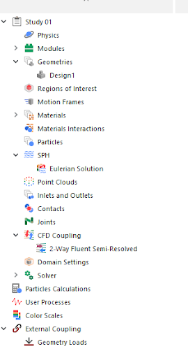
When opening Rocky, the CFD Coupling entry at the Data Tree has the 2-Way Fluent Semi-Resolved mode selected.
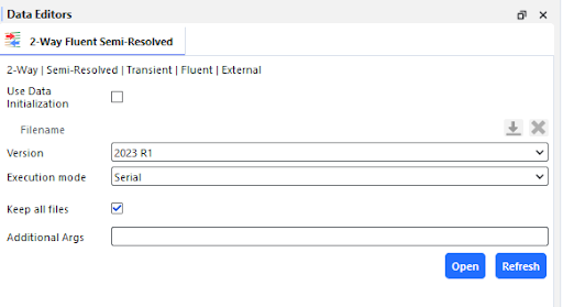
In the 2-Way Fluent Semi-Resolved Data Editor, the coupling setup can be edited as usual.
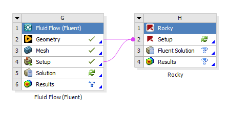
For sharing the geometry between projects, link the geometry between the Fluid project and the Rocky Setup projects. Doing so, the geometry will be automatically imported into Rocky.
For the Semi-Resolved coupling, fluid data cannot be post-processed in Rocky. For post-processing fluid data, add a new Results component system and link it to the Rocky project Fluent Solution.
Rocky's integration with Ansys Mechanical enables Mechanical to conduct either transient or static structural analyses based upon the particle forces that Rocky calculates. These two tools can operate as connected components within Ansys Workbench, or the DEM portion can be done separately in Rocky and the results later imported into Workbench for the structural analysis portion.
This section covers the following topics:
1-WAY COUPLING WITH MECHANICAL
2-WAY THERMAL COUPLING WITH MECHANICAL
2-WAY STRUCTURAL COUPLING WITH MECHANICAL
1-WAY COUPLING WITH MECHANICAL
Ansys Products needed: Ansys Rocky and Ansys Workbench
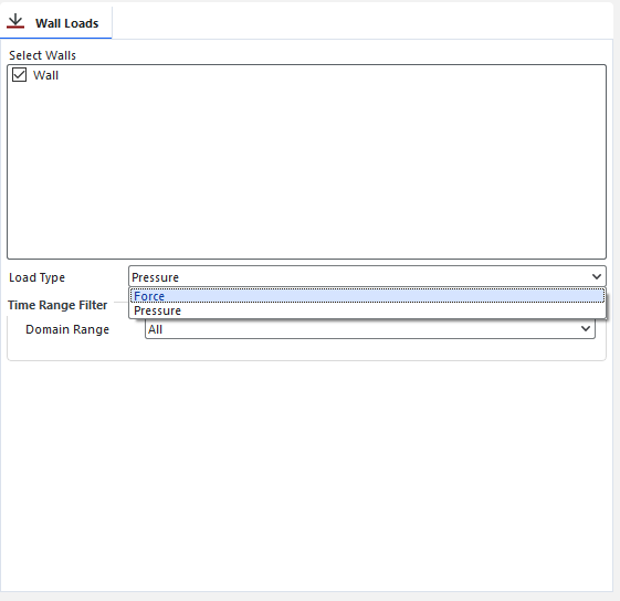
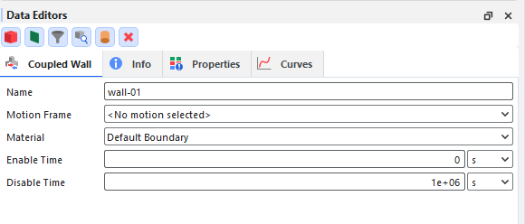
For projects coupled specifically with Ansys Mechanical, opening the Wall Loads in the Data Editors panel enables you to select which Rocky data items you want transferred to the Workbench connected Mechanical program.
For example, you can select which Walls you want to analyze in Mechanical, i.e, which loads are to be transferred and which load type you want between Force and Pressure.
See the image below:
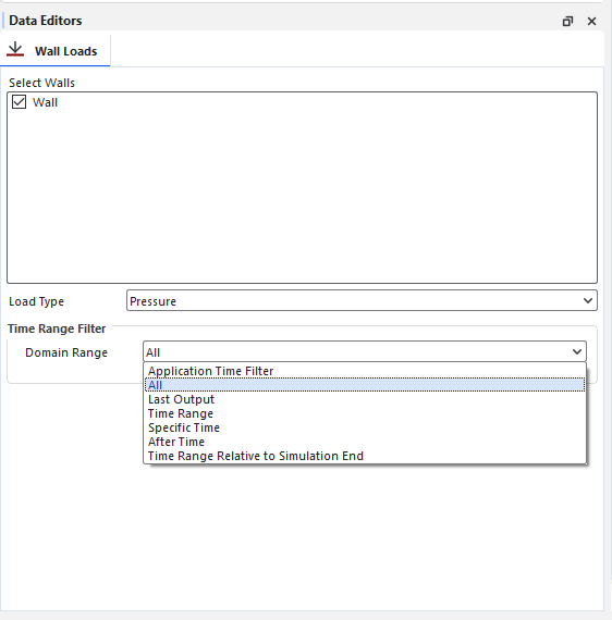
You can then select the results domain of the analysis that will be exported by setting the time range.
Important: When making a 1-way coupling with Mechanical (both 1-Way HTC and 1-Way Static and Transient Structural) the connection between Rocky Geometry and Results to Mechanical Geometry and Setup must be done manually, instead of dragging the Mechanical system and dropping it on top of the Rocky one. Otherwise, the coupling may not occur properly. This process is needed because now, for both 1-Way Static and Transient Structural (Forces only) and 1-Way HTC coupling between Rocky and Mechanical, the data from Rocky are automatically sent to Mechanical, and the manual process to copy and paste the .csv results inside Mechanical is no longer needed. For Pressure in the 1-Way Static and Transient Structural, the copy and paste is still needed.
2-WAY THERMAL COUPLING WITH MECHANICAL
[HOW-TO VIDEO]Ansys Rocky: 2-Way Thermal Coupling with Mechanical: https://www.youtube.com/watch?v=DKuTeF6eDG4&list=PL0lZXwHtV6Omiv62KRuPbnZ4oBK8BmDit&index=10
Ansys Products needed: Ansys Rocky, Ansys Mechanical, Ansys Workbench, System Coupling and Ensight.
With this coupling is possible to send heat from Rocky and receive back the temperature from Mechanical using the System Coupling.
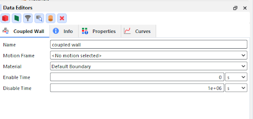
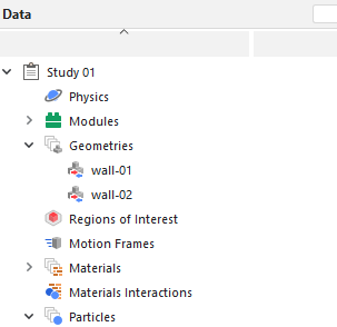
To do this, the users are able to create a coupled wall inside Rocky and the System Coupling will identify this walls as regions where the coupling is going to happen.
Limitations:
The coupled walls cannot have:
Motion Frame
Translation
Rotation
Mass tab
Wear tab
Replication tab
1- SETUP IN ANSYS ROCKY
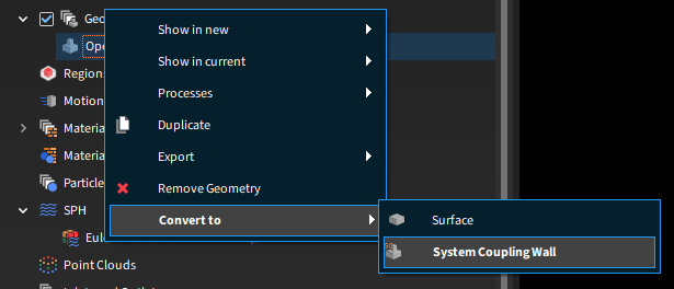
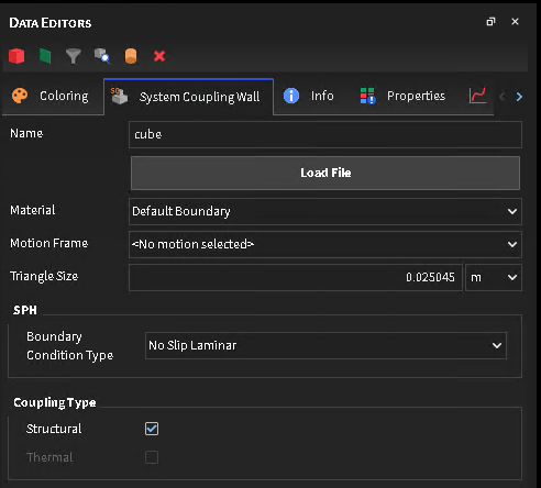
Set up your simulation as you wish, then you will have to stipulate within Rocky which geometry of your simulation you want to couple.
To do this, right-click on the desired geometry, then click on Convert to and then on System Coupling Wall.
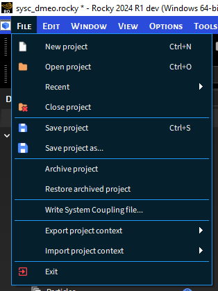
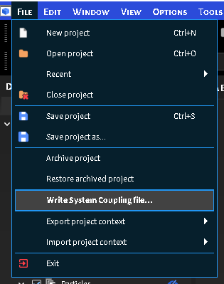
Click on File and then on Write System Coupling file. This step creates a file with information about where your Rocky file is for System Coupling.


2- SETUP IN ANSYS MECHANICAL
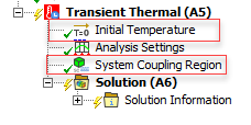
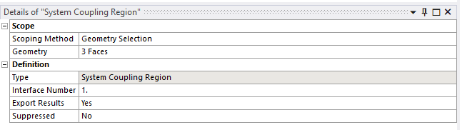
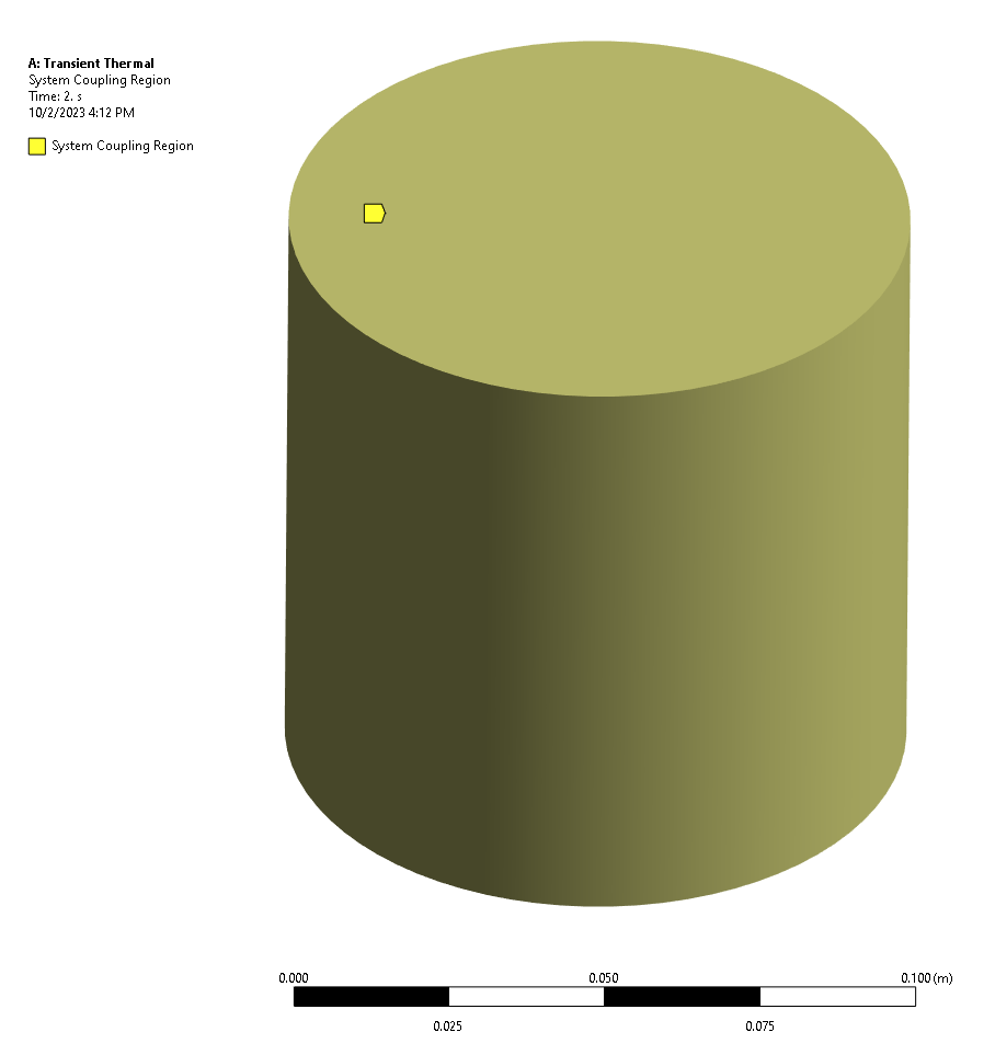
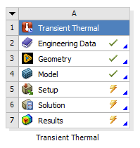
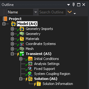
Open your project in Ansys Mechanical and set the Initial Temperature and the System Coupling Region using the Transient Thermal option.
Set the System Coupling Region, as shown in the figures below:
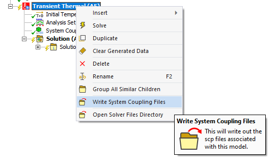
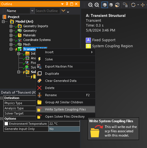
Export the System Coupling File, by right-clicking on Transient Thermal and then on Write System Coupling Files.
3- SETUP IN ANSYS WORKBENCH (TRANSIENT THERMAL)
Open your project in the Ansys Workbench and set the 2-way Thermal Coupling using the Transient Thermal option.
Learn more at About Rocky and Ansys Workbench Integration
4- SETUP SYSTEM COUPLING
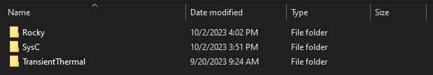
Open System Coupling and select a folder of your choice.
Tip: When you are doing this coupling, it is advisable to create three folders for your project, one for Rocky, another for Workbench and another for System Coupling.
Note: When add the folder some Warnings will appear in the message tag, but they will be resolved as you do the setup.
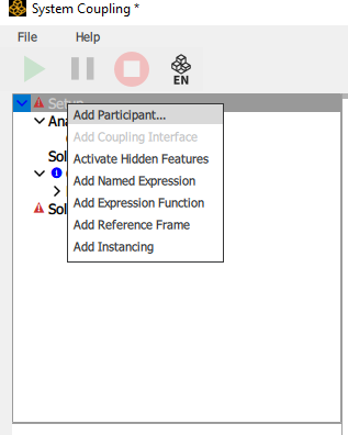
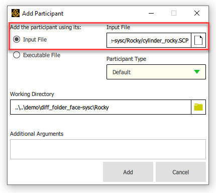
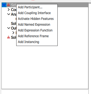
In the Data Panel, right-click Setup and then click Add Participant.
In the Add Participant window, select Input File and add the System Coupling File (.SCP) you saved from Rocky.
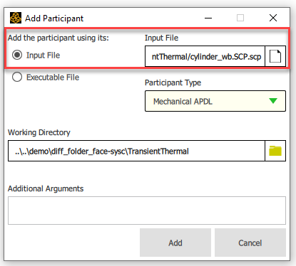
Repeat step 1, and in the Add Participant window, select Input File and add the System Coupling File (.SCP) you saved from Mechanical.
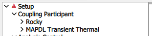
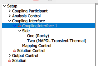
Your Data Panel must have both Rocky and Mechanical files:
In the Data Panel, right-click Setup and then click Add Coupling Interface.
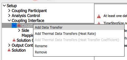
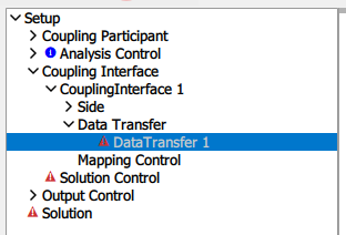
Right Click on Coupling Interface and then click on Add Data Transfer.
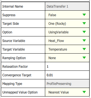
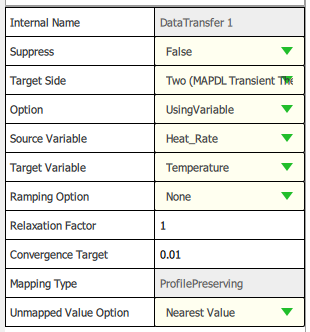
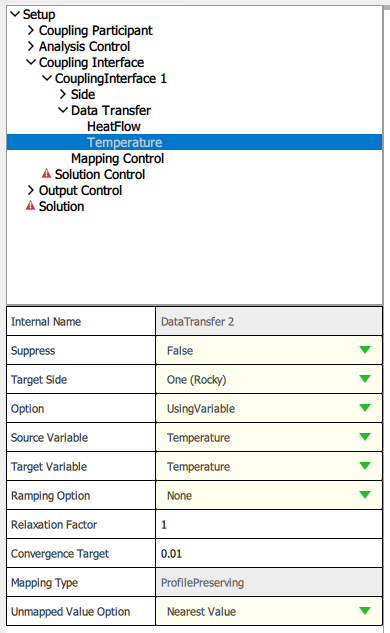
Set the Data Transfer to Rocky as show in the figures below:
Repeat step 6, and set the Data Transfer to Mechanical as show in the figures below:
In the example below the Rocky Data Transfer is named as Temperature and the Mechanical Data Transfer is named as Heat Flow:
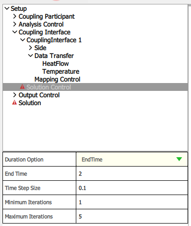
In Solution Control define the End Time and the Time Step Size.
Important: The same End Time and Time Step Size that you add in Rocky and Mechanical, you must add in System Coupling.
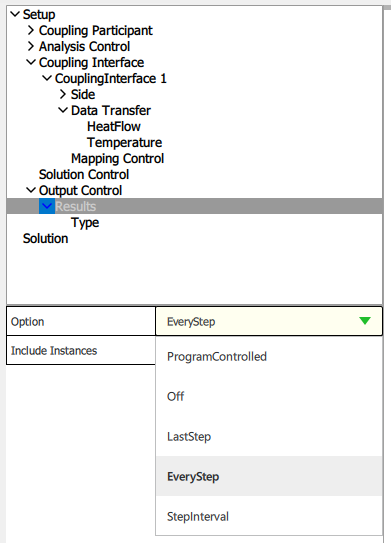
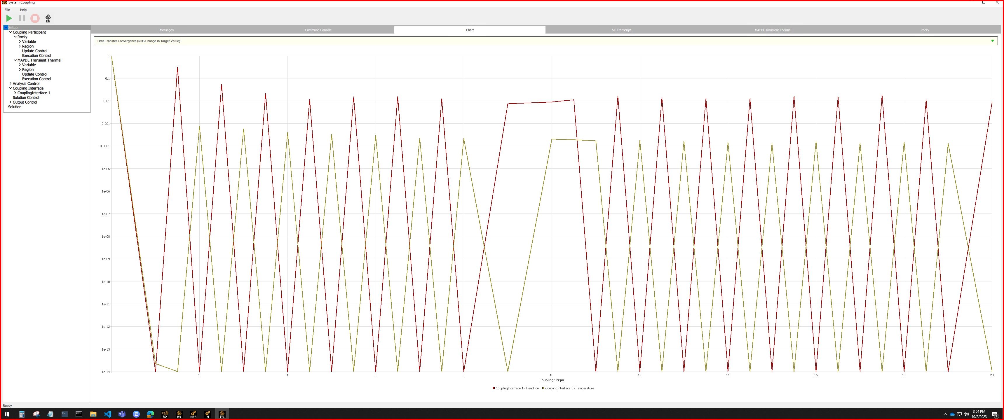
In Output Control, click on Results, and then on Type and select the Every Step option, as shown in the figure below:
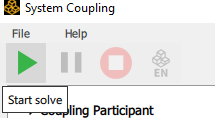
Click on Start Solve.
5- POST PROCESSING ENSIGHT
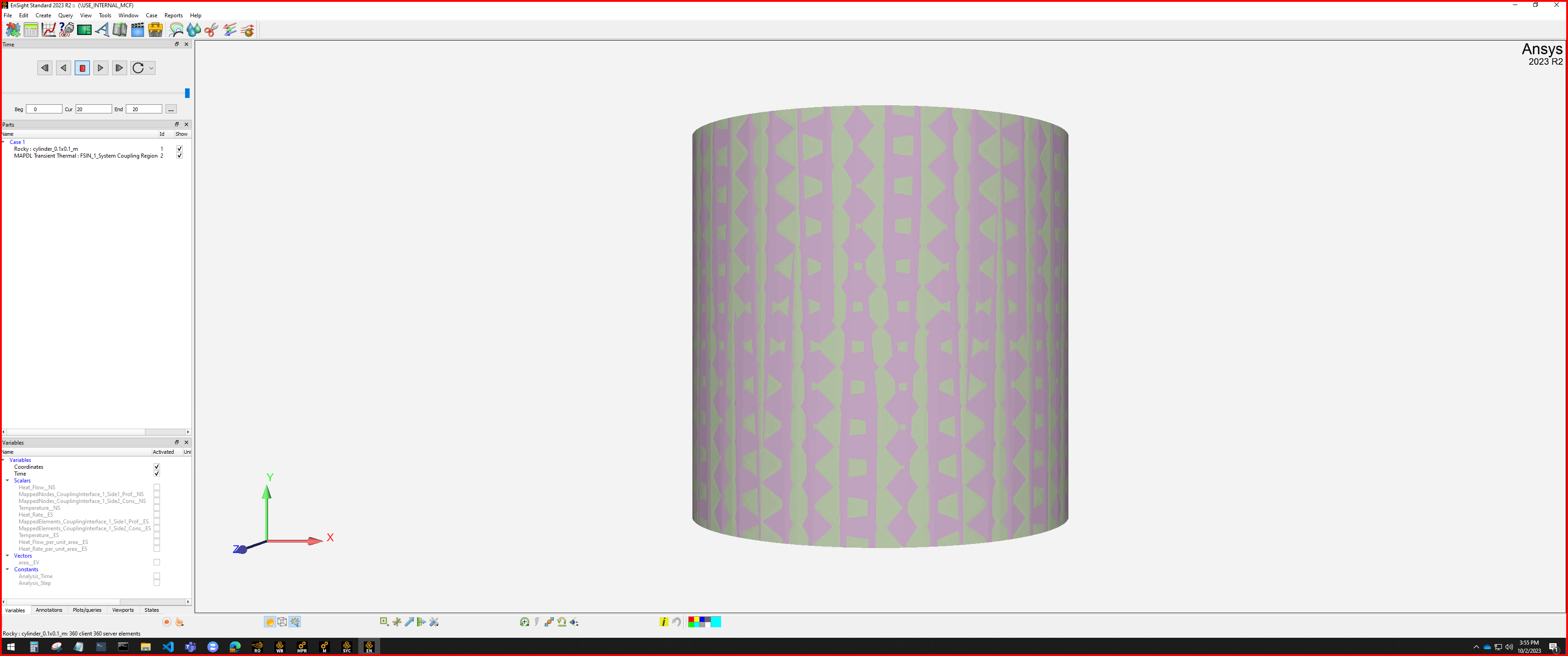
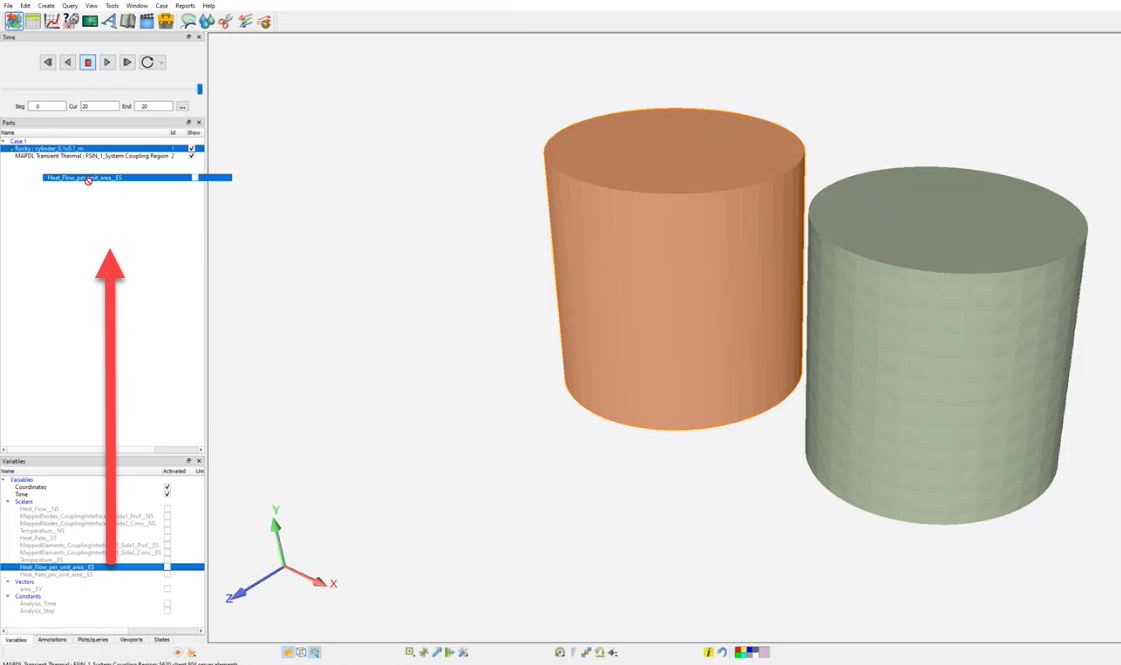
After solving your simulation, the post processing fase is carried out using the EnSight. Click on EnSight:
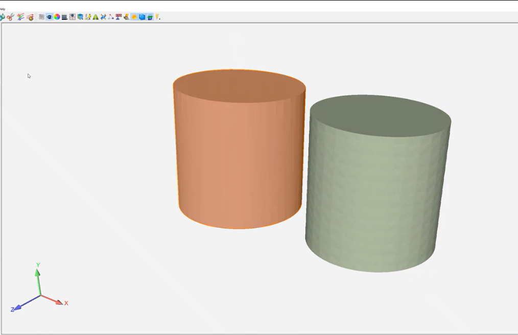
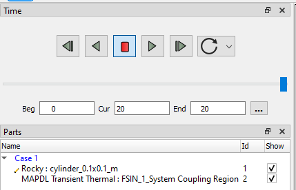
The geometries will appear in EnSight as shown in the figure below, one on top of the other, if you prefer you can separate them:
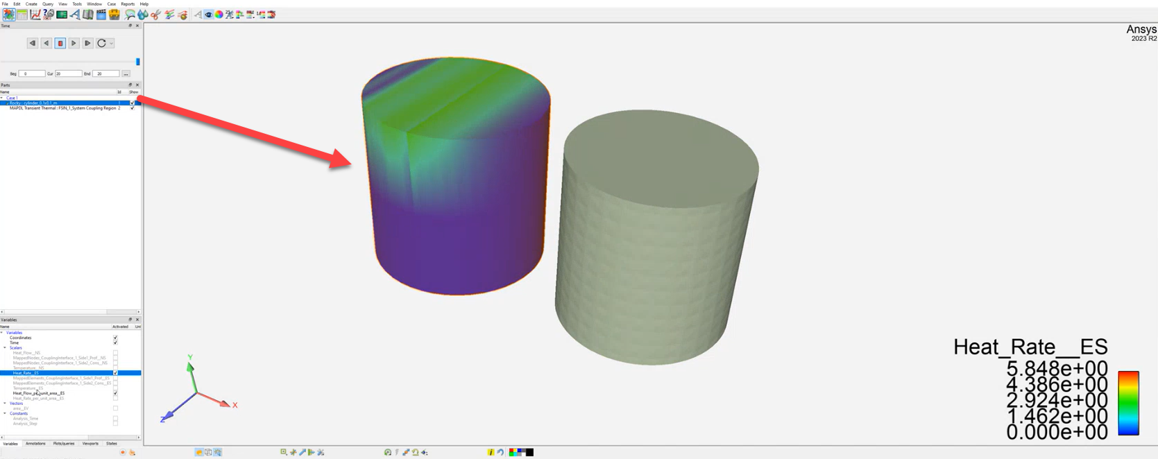
To see the results you have to drag the desired parameter to the geometry you want to see the result:

See Also:
2-WAY STRUCTURAL COUPLING WITH MECHANICAL
[HOW-TO VIDEO] Ansys Rocky: 2-Way Structural Coupling with Mechanical: https://www.youtube.com/watch?v=e89dBSdWarM&list=PL0lZXwHtV6Omiv62KRuPbnZ4oBK8BmDit&index=12
Ansys Products needed: Ansys Rocky, Ansys Mechanical, Ansys Workbench, System Coupling and Ensight.
With this coupling, it is possible to send forces from Rocky and receive back the boundary displacement from Mechanical using the System Coupling.As the 2-Way Thermal coupling between Rocky and Mechanical (using the Transient Thermal one), the 2-Way Structural coupling uses the Transient Structural System inside Workbench. The main setup process is the same as already explained for the Thermal one, with just simple differences, that will be shown below.
1- SETUP IN ANSYS ROCKY
For the Rocky side, the first difference is that now, there are 2 Coupling Types options for the System Coupling Wall. For the 2-Way Structural Coupling, just select the Structural one. And for the 2-Way Thermal, just select the Thermal one.
The rest of Rocky setup, as well the Write System Coupling file is the same as 2-Way Thermal.
2- SETUP IN ANSYS MECHANICAL
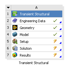
The difference from the Mechanical side is that now, the Transient Structural system for the Workbench that will be needed, as show in this image
The Model data tree setup process follows the same default Structural one, with just the System coupling regions as already described for the Thermal.
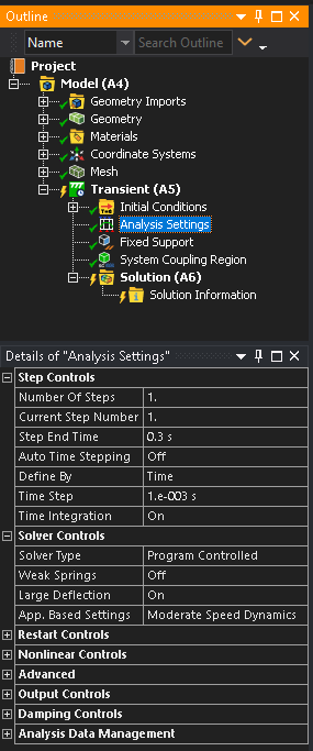
One important point here is that the Time Step inside the Analysis System, for most of the cases, will need to have a small number, as the DEM-SPH collisions will happen in a small-time fraction, and as Mechanical is an Implicit Solver, the Time Step here will need to be smaller. With the biggest time steps, Mechanical will not be able to converge, and a High Element Distortion message will be shown in the System Coupling UI.
After the setup, the System Coupling Region must be exported.
4- SETUP SYSTEM COUPLING
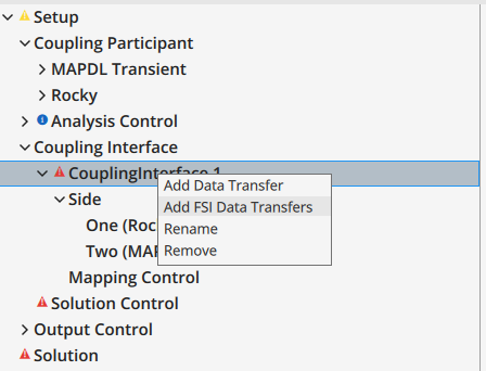
For the System Coupling side, all first steps are still the same. The only difference will be at Add Data Transfer, which now will have the Add FSI Data Transfer, which mainly will connect the forces data from Rocky, and send it to Mechanical.
Tip: When you are doing this coupling, it is advisable to create three folders for your project, one for Rocky, another for Workbench and another for System Coupling.
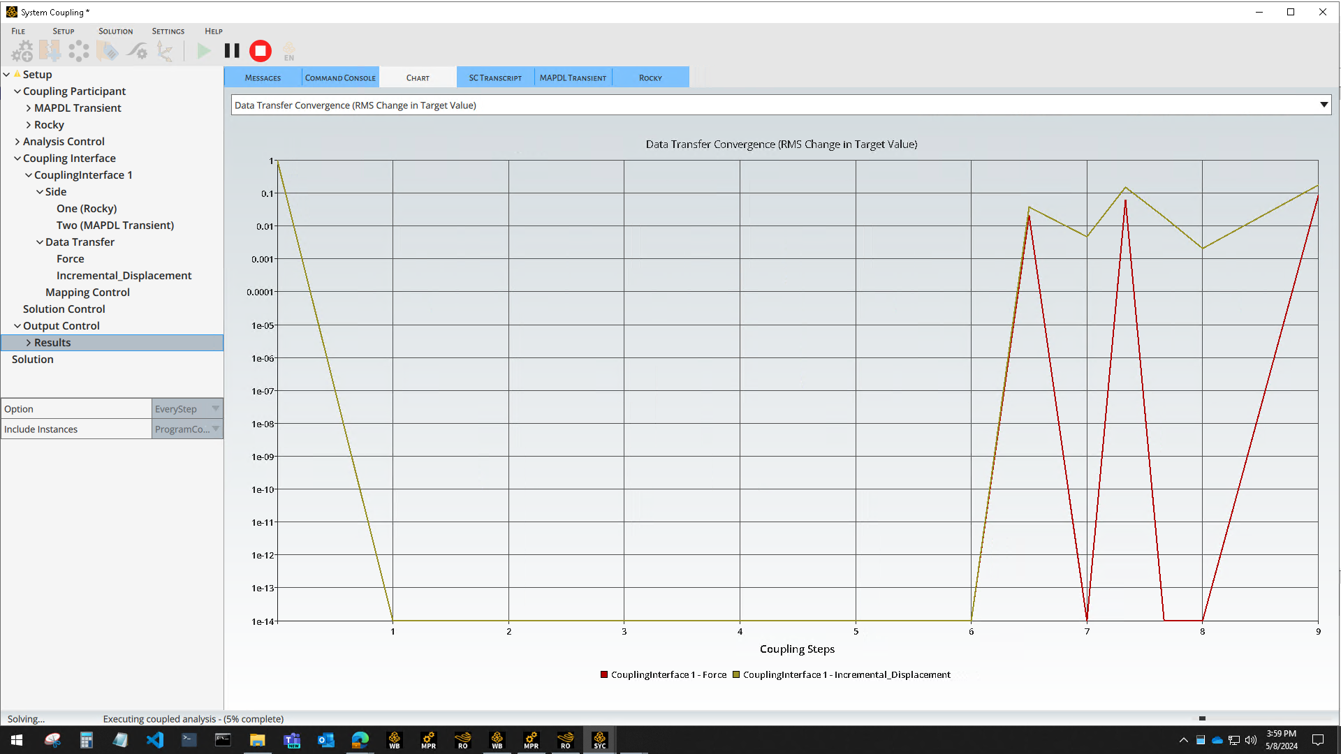
During the System Coupling solve process, it will be noticed that now, the Data Transfer will be the Force (Rocky to Mechanical) and Incremental Displacement (Mechanical to Rocky).
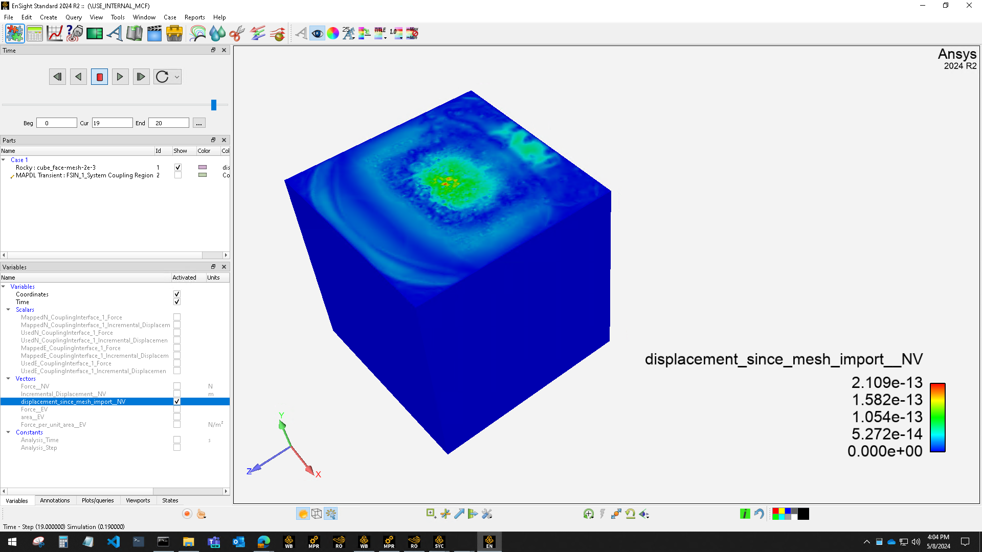
In the latest part, which is the post-processing, the two options remain: use Ensight directly from the System Coupling UI, or open Rocky and analyze the DEM-SPH trajectory and the Displacement results. At Ensight, new Variables are available, such as Force, Incremental Displacement, and Displacement Since Mesh Import, and for the Rocky side, the Displacement property will show up.
See Also:
Rocky's integration with Ansys Fluent in a 1-way coupled scenario enables Rocky to accept fluid flow and/or thermal property data from Fluent and then use that data to predict the resulting particle flow and/or related thermal properties. In a 2-way coupled scenario, Fluent and Rocky exchange fluid flow, particle forces, and thermal property data on a continual basis to discover how each interaction affects the other.
These two tools can operate as standalone products (for either 1-way or 2-way coupling) or can operate as connected components within Ansys Workbench (for 1-way coupling). But in order to make use of Fluent, an Ansys Coupling Component must be installed. (See also Install Ansys Coupling Components.)
This section covers the following topics:
IROCKY AND FLUENT BOUNDARY THERMAL COUPLING
ROCKY AND FLUENT BOUNDARY THERMAL COUPLING
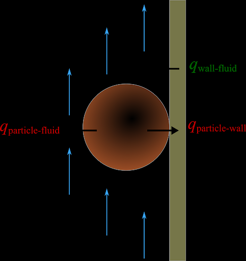
Rocky 23R1 allows the computation of the heat transfer between particles and walls. For 2-way unresolved simulations, the heat exchange during collisions is transferred to the CFD solver and used to update the surface temperature. That way, the temperature of each boundary triangle is not predefined in Rocky, but is imported from the CFD solver at every time step.
For both 1-way and 2-way coupled simulations, the particle temperature is computed by Rocky accounting for the conductive heat transfer during collisions against walls and against other particles, as well as for the convective heat exchange with the fluid phase.
For 2-way coupled simulations, the boundary temperature changes are computed by the CFD solver accounting for the heat transferred to/from the fluid phase and the heat exchanged with the particles during particle-wall collisions.
For 1-way coupled simulations, the wall temperature changes according to the CFD solution exported to Rocky (and can vary spatially and in time), but the heat exchanged during particle-wall collisions is not transferred to the CFD solver.
The coupled boundaries are automatically imported from the Fluent setup by selecting the desired walls from a list of compatible walls automatically populated in the CFD Coupling Boundaries tab.
These are the requirements for setting up a thermally coupled simulation.
The Rocky setup must have the Thermal model enabled.
The Fluent setup must have the Energy Equation turned on.
For 2-way coupled simulations, the walls must have Shell Conduction enabled in the Fluent setup, regardless of the Thermal Conditions option chosen.
Giving the wall thickness (thin wall model) but not turning on the shell conduction model does not make the wall compatible with the coupling.
Only walls in participating fluid domains can be thermally coupled to the DEM solution.
Mesh motion is not supported for thermally coupled boundaries.
Dynamic meshes (deforming meshes and remeshing) are not supported.
Polyhedral meshes are not supported.
To set up a Thermal Coupled Simulation, follow the steps below:
Import the Fluent case file and set up the required models listed in the Interactions, Coupling, Zones and Interfaces, Fluent and Variables tabs, as required for any 2-way coupled simulation.
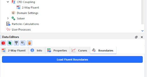
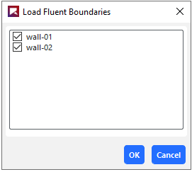
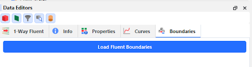
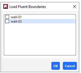
Click the 2-Way Fluent entry in the Data Panel and navigate to the Boundaries tab in the Data Editors. Clicking on Load Fluent Boundaries will open a window listing all the compatible boundaries.
Tip: Check the Requirements entry to understand the compatibility criteria.
Select the walls you want to use for the thermal coupling.
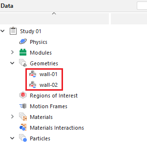
For each selected wall, a new entry will appear under Geometries in the Data panel. These walls have specific icons as they are thermally coupled.
Unselecting the wall from the Load Fluent Boundaries list will remove the coupled wall from the Geometry list, as well as any user process linked to the coupled wall.
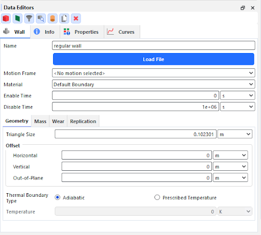
The coupled walls have fewer options compared to the standard walls as some models are not supported, such as wear and replication.
Select the Material to be assigned to the coupled wall.
Important: The mechanical properties of the assigned material will be used for computing contact forces for collisions between the particles and the wall, but the thermal properties required for the conductive heat transfer calculation will be extracted from Fluent.
Run the coupled simulation normally.
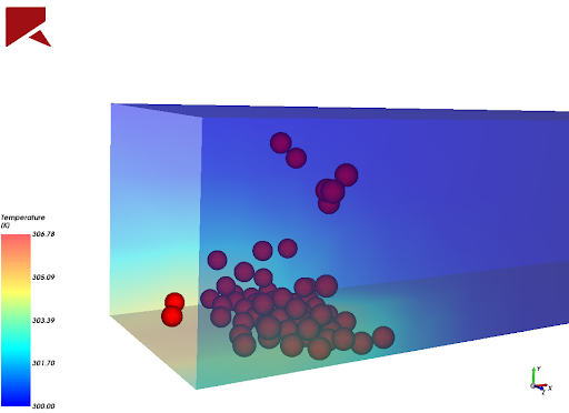
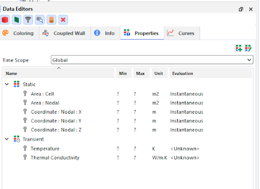
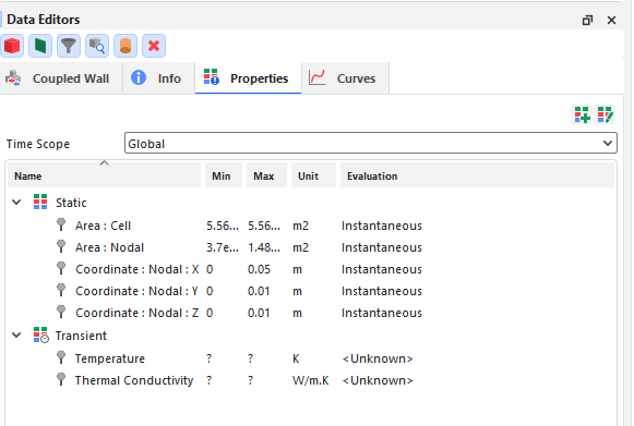
Two additional transient properties are available for coupled walls - Temperature and Thermal Conductivity. These triangle properties can be shown in 3D views or used to generate quantitative analyses such as time plots, histograms, or output parameters.
Figure 2.130: The wall temperature, initially at 300K, increases as hot particles (500K) collide with the wall.
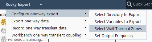
For setting up a 1-way thermal coupled simulation, there is only one additional step that must be completed. In the Rocky Export plugin, select Configure one-way export and then Select Wall Thermal Zones.
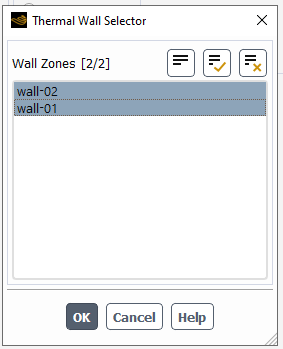
The Thermal Wall Selector window will list all the walls that are compatible with the 1-way thermal coupling between Rocky and Fluent.
Figure 2.132: List of all the walls compatible with the 1-way thermal coupling between Rocky and Fluent in the Thermal Wall Selector window.
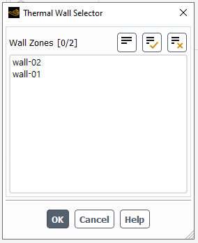
Pick the walls that you wish to participate as coupled walls.
Run the simulation normally and export the results to Rocky using the Rocky Export Plugin.
In Rocky, enable Thermal and select Fluent (Fluid -> Particle) as the coupling mode.
Select the F2R file that was exported from Fluent. Set up the required models listed in the Interactions and Coupling tabs, as required for any 1-way coupled simulation.
Click the 1-way Fluent entry in the Data Panel and navigate to the Boundaries tab in the Data Editors.
Clicking on Load Fluent Boundaries will open another window listing all the compatible boundaries. Tip: Check the Requirements entry to understand the compatibility criteria.
Select the walls you want to use for the thermal coupling.
For each selected wall, a new entry will appear under Geometries in the Data panel. These walls have specific icons as they are thermally coupled.
Unselecting the wall from the Load Fluent Boundaries list will remove the coupled wall from the Geometry list, as well as any user process linked to the coupled wall.
The coupled walls have fewer options compared to the standard walls as some models are not supported, such as wear and replication.
Select the Material to be assigned to the coupled wall.
Important: The mechanical properties of the assigned material will be used for computing contact forces for collisions between the particles and the wall, but the thermal properties required for the conductive heat transfer calculation will be extracted from Fluent.
Run the coupled simulation normally.
Additional properties are created for the coupled walls. These can be used for quantitative analyses, such as time plots and histograms, for creating output parameters or for coloring the wall triangles in a 3D view.

The ways in which Rocky and Ansys Fluent can work together are covered in the following topics:
See Also:
In version 2025 R1 of Rocky, the coupling with Ansys Motion was included into an embedded module. By doing this, the Rocky module for FMU Coupling from the Ansys Motion Coupling installer was removed. A built-in Rocky module called Multibody Dynamics FMU Coupling was created.
The Ansys Motion Coupling installer will only install the FMU Export extensions for Ansys Motion. To run a coupled simulation with any FMU file, the user must enable the Multibody Dynamics FMU Coupling Rocky module. Another detail is that the user won't need to install the modules for each user on the same machine anymore.
For additional details regarding the Ansys Motion Coupling can be found in the Installation Guide.
See Also:
Improved integration between Ansys optiSLang and Ansys Rocky can boost your iterative design processes. By combining your Ansys Rocky cases with the robust design optimization (RDO) methods of optiSLang, processes requiring many repeat runs--such as those for material calibration--get faster and more efficient. And when combined with the powerful parametric modeling capabilities of Ansys Workbench, you can take these efficiencies even farther.
Using the optiSLang plug-in, the input parameter selection and variation for your Rocky projects are automatic based upon sensitivity analyses and meta-modeling techniques. These automatic methods reduce the number of iterative cases that need to be run and increase the confidence with which you can adjust the interaction parameters for your calibration projects.
Important: Before you begin, ensure that the Rocky project you want to integrate with optiSLang has already been processed in Rocky and has simulation results. And if you only have one license of Rocky, ensure that your Rocky program is closed as optiSLang will need to open it as part of the integration process.
It is possible to integrate Ansys optiSLang with Ansys Rocky, as show below:
Open the Ansys optiSLang program.
From the main Ansys optiSLang screen, under New Project, click Guided (as shown) to open the Solver Wizard.
From the Solver Wizard, search for Rocky, and then under Interfaces, select the ROCKY option (as shown).
From the Select project file dialog, navigate to and then select the already-processed Rocky project file you want to use, and then click Open (as shown).
. From the Choose Rocky script to export results dialog, select the script (.py) file you want optiSLang to use for the exported output variables, and then click Open (as shown).
Note: By default, optiSLang creates .py files for this purpose in the same folder as the Rocky project you selected earlier. After optiSLang loads the input/output variables, Rocky will launch and you will receive a confirmation message.
Tip: For more information about using optiSLang, refer to the Ansys/Dynardo optiSLang User Documentation.
See Also:
For more information about Rocky integration with Ansys Minerva, refer to the information on the Installation Guide. https://innovationspace.ansys.com/ais-rocky/.
See Also: