


Whether you are beginning a new simulation or modifying an existing one, it is a good idea to ensure that your simulation parameters are set exactly the way you want before you start processing. Once you Start a Simulation and begin processing, you cannot go back and change the settings without losing the simulation results that have been created.
Setting simulation parameters involves setting simulation-wide values as well as parameters specific to particles, geometries, materials, interactions, inputs, and more. To make the setup of multiple similar items quicker, you many also choose to duplicate already-setup items, or remove many similar items at one time.
What would you like to do?
See Also:
You set simulation-wide parameters when you want to change the default values provided by Rocky to affect your whole simulation. Simulation-wide parameters are settings that can include:
Study items, which include setting the simulation title and customer name.
Physics items, which include setting how you want gravity applied; and setting simulation-wide models such as adhesion, rolling resistance, heat transfer, and coarse graining.
Modules items, which include collision and particle statistics collection.
Domain Settings items, which include defining the simulation coordinate limits and setting an optional periodic domain.
Solver items, which include setting simulation time length, and certain data collection times.
Simulation-wide parameters are set by first selecting the Study, Physics, Modules, Domain Settings, and Solver sections in the Data panel and then editing the results in the Data Editors panel. These values can be set at any time before you begin processing your simulation. However, it is recommended that at least the Physics and Modules settings be made first as your selections there may affect other settings later on.
What would you like to do?
Learn more About Study Parameters
Learn more About Physics Parameters
Learn more About Modules Parameters
Learn more About SPH Parameters
Learn more About Domain Settings Parameters
Learn more About Solver Parameters
Set Study, Physics, Modules, Domain Settings, and Solver Parameters
See Also:
Note: Unlike most other setup parameters, you are able to change your Study parameters at any time-even during active processing. (See also I cannot change my setup parameters during processing.)
Use the figures and table below to help you understand the various Study parameters you can set for a simulation project.
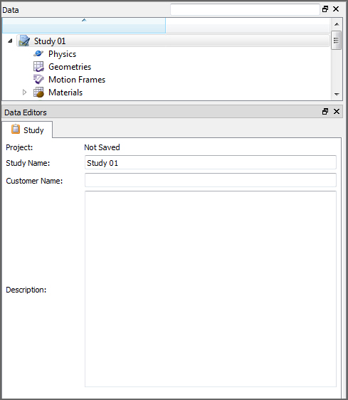
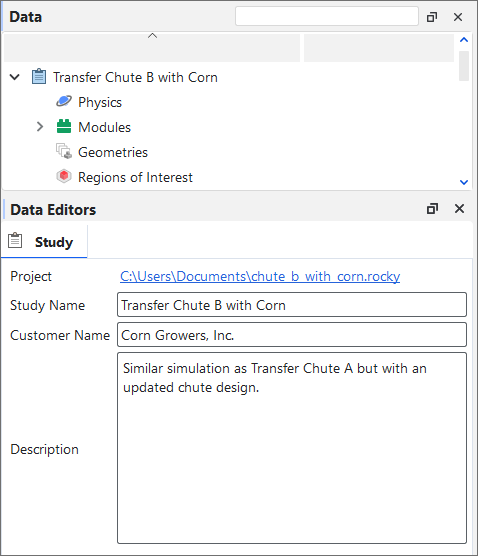
Table 1: Study parameter options
Setting | Description | Range |
|---|---|---|
Project | When the project is saved, this lists the full path for the .rocky project file in hyperlink form (Figure 2). If the project has not yet been saved, "Not Saved" will be displayed (Figure 1). | Path automatically provided |
Study Name | Name of the simulation you are working on. For example, "Transfer Chute B with corn." Note: The Study entity on the Data panel will be renamed with what you enter here (Figure 2). | No limit |
Customer Name | Name of the customer for whom you are doing the simulation. | No limit |
Description | Description of the simulation. | No limit |
What would you like to do?
See Also:
The Rocky Physics parameters include simulation-wide settings that affect how the components are calculated. These include settings affecting gravity; the rolling resistance and force models used for calculating momentum; and the separate settings that enable Thermal Modeling and Coarse-Graining.
The rolling resistance and force models used for calculating momentum have specific combinations that are unsupported in this version of Rocky. Refer to the compatibility table in Physics and Force Limitations for details.
To learn more about how these models are calculated, refer to the DEM Technical Manual. (From the Rocky Help menu, point to Manuals and then click DEM Technical Manual.)
To learn more about setting up and using Thermal in Rocky, refer to the Enable Thermal Modeling Calculations topic.
To learn more about how this model is calculated, refer to the DEM Technical Manual. (From the Rocky Help menu, point to Manuals and then click DEM Technical Manual.)
To learn more about the Coarse-Graining used in Rocky, and see examples for its usage, refer to the following resources:
DEM Technical Manual. (From the Rocky Help menu, point to Manuals and then click DEM Technical Manual.)
CFD Coupling Technical Manual. (From the Rocky Help menu, point to Manuals and then click CFD Coupling Technical Manual.)
In this version of Rocky, Coarse-Graining and Particle Breakage are incompatible. This means if any Particle sets within an Enable Coarse-Graining (previously named Coarse Grain Modeling (CGM)) simulation has breakage parameters enabled, the entire simulation-including any Particle sets without breakage-will be unable to be processed.
In addition, CGM works only with single-element particle shapes. This means that Coarse Grain Models are incompatible with Particle sets composed of multiple elements (also known as Meshed particles), including flexible Fibers, flexible Shells, and flexible Solids.
In terms of momentum settings, CGM can be used only with these two Adhesive Forces: Constant and Linear. All other types of Adhesive Forces-including JKR-are incompatible with Coarse Grain Modeling in this version. Also note that the Velocity Dependent restitution model (an Experimental (Beta) Feature) is also incompatible with CGM.
In terms of CFD coupling, Coarse Graining is incompatible with 1-Way LBM. While other types of coupling is allowed, only drag forces will be considered. This means that fluid forces such as torque, virtual mass, and lift are not compatible with Coarse Graining. (See also the CFD Coupling Technical Manual. (From the Rocky Help menu, point to Manuals and then click CFD Coupling Technical Manual.))
Also note that the Radl et al. Coarse Grain Model is currently incompatible with Multi GPU processing. (It is compatible with both Single GPU and CPU processing, however.)
(See also Physics and Force Limitations.)
Use the figures and table below to help you understand the various Physics parameters you can set for a simulation project.
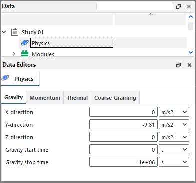
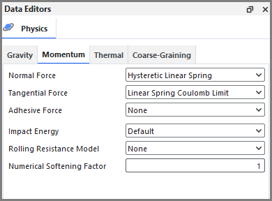

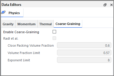
Table 1: Physics parameter options (all tabs)
Setting | Description | Range |
|---|---|---|
Gravity | ||
X-direction | Used to change the direction that gravity affects particles and free boundaries, this is the amount of acceleration applied in the X direction during the simulation. Tip: When prescribing movements, it can be easier to align geometries with the global axes and then simulate gravity in the plane that represents downward forces. For example, if you had your equipment horizontally aligned with the X direction, you could then modify the Y and X components of gravity to simulate it as if it were inclined in the YX plane. | No limit |
Y-direction | Used to change the direction that gravity affects particles and free boundaries, this is the amount of acceleration applied in the Y direction during the simulation. Note: The default value is -9.81 m/s2, which accounts for the effect of gravity pointing in the downward Y direction only. | No limit |
Z-direction | Used to change the direction that gravity affects particles and free boundaries, this is the amount of acceleration applied in the Z direction during the simulation. | No limit |
Gravity Start Time | The duration you want to wait before gravity components are activated. | Positive values |
Gravity Stop Time | The duration you want to wait before gravity components are deactivated. | Positive values |
Momentum | ||
Normal Force | The type of model used to calculate the normal components of the contact forces. The model you select here determines what Adhesive Force and Tangential Force options are available. For additional details about these models, see the Rocky DEM Technical Manual. (From the Rocky program Help ** menu, point to **Manuals, and then click DEM Technical Manual.) | Hysteretic Linear Spring; Linear Spring Dashpot; Hertzian Spring Dashpot Note: This setting is considered to be exclusive so if you have one or more external Modules that are able to override this model, you must have only one such Module enabled within your simulation project. Refer to the Module's documentation (if provided) for more information. (See also Rocky Simulation Entities that can be Affected by Modules.) |
Tangential Force | The type of model used to calculate the tangential components of the contact forces. The models available are dependent upon the Normal Force you selected. Specifically:
For additional details about these models, see the Rocky DEM Technical Manual. (From the Rocky program Help ** menu, point to **Manuals, and then click DEM Technical Manual.) | Linear Spring Coulomb Limit; Coulomb Limit; Mindlin-Deresiewicz Note: This setting is considered to be exclusive so if you have one or more external Modules that are able to override this model, you must have only one such Module enabled within your simulation project. Refer to the Module's documentation (if provided) for more information. (See also Rocky Simulation Entities that can be Affected by Modules.) |
Adhesive Force | Defines how adhesion between materials is calculated. Material-to- Material interactions are then defined in the Modify Material Interaction and Adhesion Values step. (See also About Modifying Materials Interactions and Adhesion Values.) The models available are dependent upon the Normal Force you selected. Specifically:
For additional details about these models, see the Rocky DEM Technical Manual. (From the Rocky program Help ** menu, point to **Manuals, and then click DEM Technical Manual.) | None; Constant; Linear; JKR Note: This setting is considered to be exclusive so if you have one or more external Modules that are able to override this model, you must have only one such Module enabled within your simulation project. Refer to the Module's documentation (if provided) for more information. (See also Rocky Simulation Entities that can be Affected by Modules.) |
Restitution Model | When the Experimental (Beta) Features checkbox is enabled on the Options | Preferences dialog (see also About Setting Global Preferences), this enables you to select the type of model used to calculate restitution. Note: The Velocity Dependent model is incompatible with Enable Coarse-Graining. (See also the Coarse-Graining section below.) | Constant; Velocity Dependent |
Impact Energy | The type of model used to calculate the impact energy of a contact. Unless you have enabled a custom external Module that defines a different Impact Energy model, the only option listed will be Default. Impact energy is used in Rocky as the main input parameter for the built-in instantaneous breakage models. You will need to implement a custom impact energy calculation only if you intend to use a custom contact force model along with such breakage models. If in that case, you choose not to implement the impact energy calculation, Rocky will use a standard calculation based on the impact work, as defined in equation (4.10) of the DEM Technical Manual. | Default Note: This setting is considered to be exclusive so if you have one or more external Modules that are able to override this model, you must have only one such Module enabled within your simulation project. Refer to the Module's documentation (if provided) for more information. (See also Rocky Simulation Entities that can be Affected by Modules.) |
Rolling Resistance Model | Defines how rolling resistance for particles are calculated. After a model is selected, Rolling Resistance values are then set per Particle sets on its Movement tab. (See also About Adding and Editing Particle Sets). Specifically:
Note: Both types of Rolling Resistance Models are incompatible with concave Custom Polyhedron particle shapes (see also Physics and Force Limitations.) For more information on the calculations used to form these models, see the Rocky DEM Technical Manual. (From the Rocky program Help ** menu, point to **Manuals, and then click DEM Technical Manual.) | None; Type A: Constant Moment; Type C: Linear Spring Rolling Limit |
Numerical Softening Factor | Factor applied to the materials (includes both particles and boundaries) stiffnesses values that are used to calculate both timesteps and contact forces. This enables you increase the size of your timesteps, and speed up your processing time, without having to change the material properties themselves. This is especially useful in long or particularly complex cases, or for those with Thermal Modeling enabled. Tips:
See also About Modifying Material Compositions and and Enable Thermal Modeling Calculations. | Positive values Note: Typical values will range between 0.001 and 1.0 |
Thermal | ||
Enable Thermal | Makes possible the simulation of conductive heat transfer between particles and other particles, and particles and boundaries. Enables convective heat transfer between particles and fluids when coupled with Ansys Fluent (see also Set or Modify Fluid and/or Air Flow Properties). See also Enable Thermal Modeling Calculations. | Turns on or off |
| Particle Settings | ||
Heat Conduction Model | When Enable Thermal is selected, this is the type of model used to calculate heat conduction. Unless you have enabled a custom external Module that defines a different Heat Conduction Model, only the default Vargas McCarthy 2002 model will be used. | Vargas McCarthy 2002 Note: This setting is considered to be exclusive so if you have one or more external Modules that are able to override this model, you must have only one such Module enabled within your simulation project. Refer to the Module's documentation (if provided) for more information. (See also Rocky Simulation Entities that can be Affected by Modules.) |
Conduction Correction Model | When Thermal is enabled, this allows you to select a strategy to counteract the adverse effects that can occur when you use the Numerical Softening Factor to speed up a simulation. (See also the definition in the Momentum tab section above.) Specifically:
Tip: To learn more about these models, refer to the DEM Technical Manual. (From the Rocky Help menu, point to Manuals and then click DEM Technical Manual.) | None; Morris et al. Area; Morris et al. Area+Time |
Thermal Integration Model | When Enable Thermal is selected, this is the type of model used to integrate heat conduction calculations. Unless you have enabled a custom external Module that defines a different Thermal Integration Model, only the default Lumped Capacitance Method will be used, which ignores any conduction inside the particle and assumes only that the entire particle has a single temperature. | Lumped Note: This setting is considered to be exclusive so if you have one or more external Modules that are able to override this model, you must have only one such Module enabled within your simulation project. Refer to the Module's documentation (if provided) for more information. (See also Rocky Simulation Entities that can be Affected by Modules.) |
| SPH Settings | ||
| Heat transfer Model |
When Enable Thermal is selected, this is the type of model used to calculate heat transfer for SPH elements. Unless you have enabled a custom external module that defines a different Heat transfer Model, only the default, Cleary model, will be used. | Cleary Note: This setting is considered to be exclusive so if you have one or more external Modules that are able to override this model, you must have only one such Module enabled within your simulation project. Refer to the Module’s documentation (if provided) for more information. |
Coarse-Graining | ||
Enable Coarse-Graining | Enables a coarse grain model (CGM) to be used in the simulation. Tip: Turning on Enable Coarse-Graining allows you to increase the original particle size and reproduce the system behavior using a reduced number of particles via use of the CGM Scale Factor. (See also the Size Tab section of About Adding and Editing Particle Sets.) Notes: In this version of Rocky, Enable Coarse-Graining is incompatible with:
| Turns on or off |
Radl et al. | When Enable Coarse-Graining is selected, this determines whether or not the Radl et al. model will be enabled, which helps describe additional physical processes on particle flows by determining the amount of energy dissipated based upon the velocities of the surrounding particles. Specifically:
Note: In this version of Rocky, the Radl et al. model is incompatible with Multi GPU processing. (See also About Starting a Simulation.) Tip: To learn more about these models, refer to the DEM Technical Manual. (From the Rocky Help menu, point to Manuals and then click DEM Technical Manual.) | Turns on or off |
Close Packing Volume Fraction | When Radl et al. is enabled, this defines the maximum volume fraction that particles are allowed to reach, which is one of three parameters that together determine what characteristics turn off the Radl et al. model and how quickly that shutoff happens. The shutoff function is especially important for cases with closely packed particles in constant contact as the Radl et al. model is not optimized for this scenario and applying it in those situations result in too much energy being removed from the system. Tip: This parameter is represented by Note: This text field does not support parametric variables. (See also I cannot enter an input variable or mathematical function into a text field.) | 0-1 |
Volume Fraction Limit | When Radl et al. is enabled, this defines the particle volume fraction value above which the shutoff function will not affect the particles' relaxation time. This parameter is one of three that together determines what characteristics turn off the Radl et al. model and how quickly that shutoff happens. The default value of 0.57 represents 95% of the default Close Packing Volume Fraction of 0.6. Tip: This parameter is represented by | 0-1 |
Exponent Limit | When Radl et al. is enabled, this defines the exponent value (default is 8) used in the shutoff function. The exponent is used to control how sensitive the shutoff function is regarding volume fraction variations, and is one of three parameters that together determines what characteristics turn off the Radl et al. model and how quickly that shutoff happens. Tip: Refer to equation 2.101 in the Rocky DEM Technical Manual for details. | 0-100 |
Search Distance Multiplier | When the Advanced Features checkbox is enabled on the Options | Preferences dialog (see also About Setting Global Preferences), and the Radl et al. checkbox is also enabled, this value will be multiplied by the biggest particle size to achieve the estimation radius used by the Radl et al. model to determine which particles are close enough to be used for energy dissipation calculations. Specifically:
| Positive values Note: This value must be greater than Update Distance Multiplier |
Updated Distance Multiplier | When the Advanced Features checkbox is enabled on the Options | Preferences dialog (see also About Setting Global Preferences), and the Radl et al. checkbox is also enabled, this value will be multiplied by the biggest particle size to define the distance a particle has to move before Rocky will update the neighbor list used by the Radl et al. model to compute the average neighbor velocity. Specifically:
| Positive values Note: This value must be less than Search Distance Multiplier |


What would you like to do?
See Also:
When you enable a Module in Rocky, you are choosing to add in custom, discrete features and/or functionality within your project. Depending upon the type of Module you enable and what it does, there may be additional settings that affect other areas of your Rocky project setup.
Use this topic to understand more about Module parameters and how setting them affect your project.
Tip: To learn more about the different types of Rocky Modules and where you obtain them, refer to the topic Understand Rocky Modules.
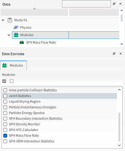
Because the default state for most Modules is disabled, it becomes very important for you to ensure that you have enabled the Modules and options you want prior to setting up the rest your simulation. This is done by selecting the main Modules entity in the Data panel and then enabling the checkbox for the module you want to use in the Data Editors panel (Figure 1).
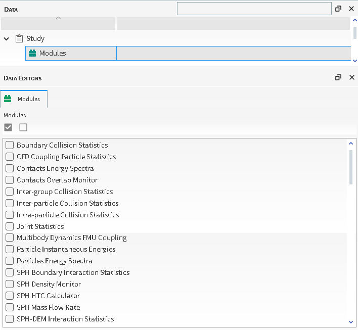
Important: Only embedded Modules and external Modules that you have already installed will appear in on the list. (See also Install an External Module.)
In addition, because it is possible that turning on a Module will add or change options presented in other parts of the Rocky setup, it is recommended that turning on the Modules and options you want is one of the very first steps you take when setting up your project.
Tip: If you have similar projects that you set up regularly, using a script to record and then play back your Module configuration steps can save you from having to repeat these steps on future projects. (See also About Creating and Using PrePost Scripts.)
Note: Enabling more than one Module at once can cause some parameters to be shared across Modules. (See also Recognize Shared Parameters with Asterisks (*).)
Once enabled, many types of Modules have parameters that you can define. Depending upon the type of Module and what it does, the settings can be in any of the following combinations.
For these types of Modules, once you enable the Module itself, the functionality will be applied without any additional actions from you.
Tip: You will know that a Module has no additional settings when you select it from the Data panel, and find no settings on the Module's Data Editors panel, and its Info tab says "Module does not affect any simulation entity."
An example of this kind of Module is the Particle Instantaneous Energies Module. (See also About the Particle Instantaneous Energies Module.)
For these types of Modules, once you enable the Module itself, there are one or more additional settings in one or both of the following locations:
On the Module's Data Editors panel
For these types of Modules, there are one or more additional settings to be made on the Data Editors panel for the Module.
An example of this kind of Module is the Boundary Collision Statistics Module. (See also About the Boundary Collision Statistics Module.)
Elsewhere in the Rocky setup
For these types of Modules, there are one or more additional settings to be made in (or have otherwise been affected by) other locations of the Rocky UI. These may require additional setup steps for the Module in those other locations.
Tip: You will know that a Module has other settings in (or is otherwise affecting) other parts of the Rocky setup when you select it from the Data panel and then from the Data Editors panel, see that its Info tab has information next to the Affected Simulation Entities label. You can then use that information to discover where else in the Rocky setup Module-specific settings might need to be applied.
An example of this kind of Module is the Liquid Bridge Model Module, which has Module-specific settings in three other areas of the Rocky setup.
Note: In this version of Rocky, the Liquid Bridge Model Module is provided as an *external* module. Refer to the Install an External Module topic for details.
Use this section to learn more about where and when you might define parameters for your Modules.
Once enabled, some types of Modules will have additional settings on the Module's main tab in the Data Editors panel. To learn if there are additional, Module-specific settings that affect other parts of your Rocky project setup, you can view the information on the Info tab.
The Info tab on individual Modules (see also About the Info Tabs) describe the Author and Version details for the Module, and lists what other entities in the Rocky UI are affected by enabling that particular Module.
For example, the Info tab for the Liquid Bridge Model Module (Figure 2) describes three places in the Rocky UI affected by that module.
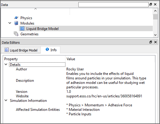
This information can help you verify that the parameters in those locations are set correctly for the feature enabled by the module.
Note: In this version of Rocky, the Liquid Bridge Model Module is provided as an *external* module. Refer to the Install an External Module topic for details.
Once enabled, some Modules will cause other areas of the Rocky UI to have additional settings specific to that Module, or will cause other changes, such as model overrides. These kinds of changes and additional settings are unique to each Module, so the best way to determine what other settings might be required for your Module is to view the Affected Simulation Entities information on the Info tab. (See the "About the Info Tab for Modules" section above.)
Once you understand what other parts of the UI are affected, you can then be sure to verify the Module-specific settings in those areas when setting up the rest of your project.
Tip: To learn more about what specific Rocky UI settings and options Modules can affect, refer to the Rocky Simulation Entities that can be Affected by Modules topic.
What would you like to do?
Learn more About Rocky Modules
Learn more About the Contacts Energy Spectra Module
Learn more About the Contacts Overlap Monitor Module
Learn more About the CFD Coupling Particle Statistics Module
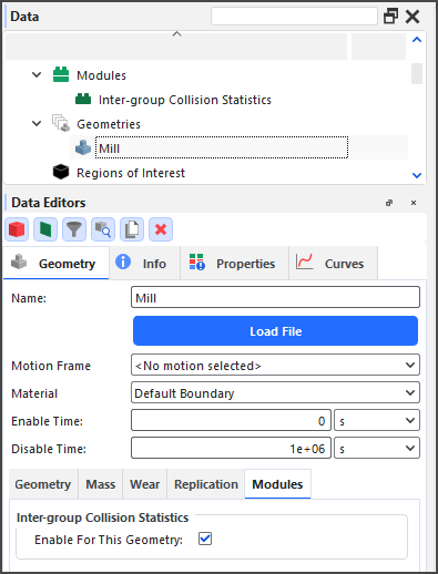
Learn more About the Inter-group Collision Statistics Module
Learn more About the Inter-particle Collision Statistics Module
Learn more About the Intra-particle Collision Statistics Module
Learn more About Joint Statistics Module
Learn more About the Particles Energy Spectra Module
Set Study, Physics, Module, Domain Settings, and Solver Parameters
See Also:
The Boundary Collision Statistics module enables the collection of boundary-related collision data, such as collision frequency, intensities, and impact velocities.
Figure 3.11: Options in the Data Editors panel when the Boundary Collision Statistics Module is enabled
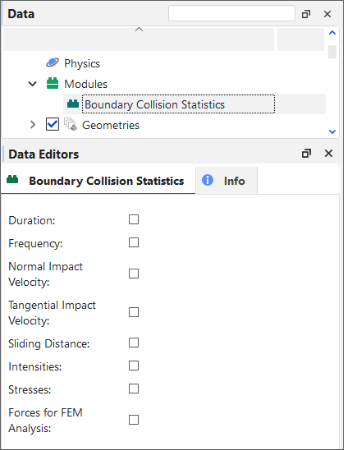
When the Boundary Collision Statistics Module is enabled (Figure 1), you are able to select any of the following Properties:
Duration
Forces for FEM Analysis
Frequency
Intensities
Normal Impact Velocity
Sliding Distance
Stresses
Tangential Impact Velocity
After processing your simulation, specific Properties and Curves for the options you enabled will be available for the boundaries in your simulation.
What would you like to do next?
The Contacts Energy Spectra module enables the collection of different kinds of energy statistics per contact pair (particle group and/or geometry) and size, which can help you predict breakage and attrition rates for continuous processes such as grinding mills.
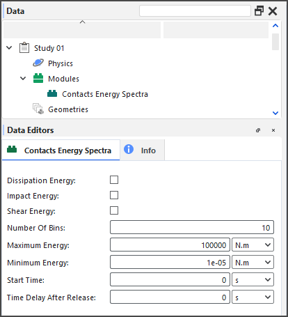
When the Contacts Energy Spectra Module is enabled (Figure 1), you can choose to collect one or more of three different types of collision energy-Dissipation Energy, Impact Energy, and/or Shear Energy-and define the limits for how the energy data is collected.
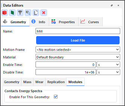
In this version of Rocky, you can also choose which particle group (Figure 2) and geometry component Figure 3.13: Additional module options for Particle groups when the Contacts Energy Spectra module is enabled you want to participate in energy spectra collection.
Figure 3.13: Additional module options for Particle groups when the Contacts Energy Spectra module is enabled
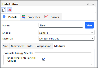
Figure 3.14: Additional module options for a geometry component when the Contacts Energy Spectra module is enabled
After processing your simulation, you can plot the resulting energy curves (Dissipation, Impact, and/or Shear) for each pair of particle-to-particle or particle-to-geometry contact types, each generated by the power, cumulative power, and collisions rate.
What would you like to do next?
When enabled, the Contacts Overlap Monitor module checks each contact pair (particle-particle or particle-boundary) for the amount that they overlapped-the percentage of which is determined by the size of the smallest particle in the contact pair-and then raises a warning in the Simulation Log panel (Figure 1) if an overlap exceeds any of the three warning levels you define (Figure 2).
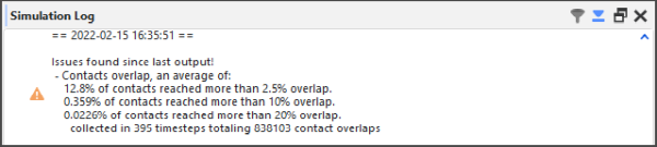
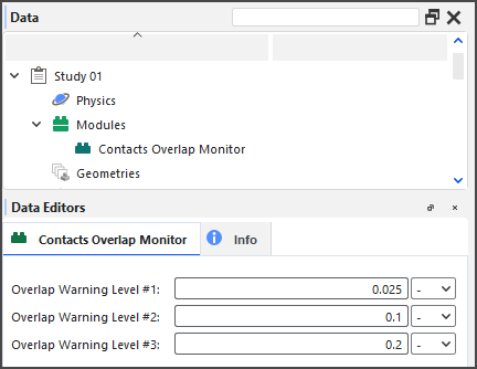
Monitoring your contacts for overlaps is important because Rocky uses the overlap value in order to compute collision forces. Therefore, large overlap values can lead to serious stability and accuracy issues in a simulation.
What would you like to do next?
Learn more About Monitoring Overlaps
Learn more About Collecting Data in Rocky
See Also:
The CFD Coupling Particle Statistics Module enables the collection of particle-fluid interactions, such as drag, lift, and virtual mass forces.
Figure 3.17: Options in the Data Editors panel when the CFD Coupling Particle Statistics Module is enabled
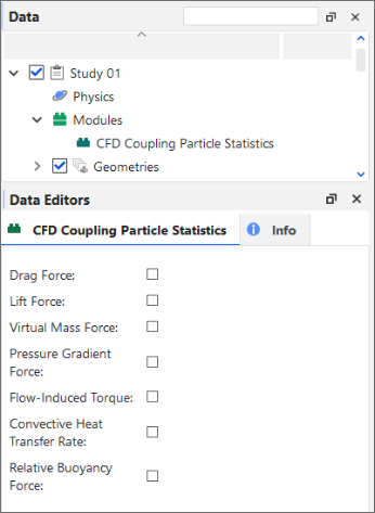
When the CFD Coupling Particle Statistics Module is enabled (Figure 1), you are able to select any of the following Properties:
Convective Heat Transfer Rate
Drag Force
Flow-Induced Torque
Lift Force
Pressure Gradient Force
Virtual Mass Force
After processing your simulation, specific Properties for the options you enabled will be available for the particles in your CFD Coupling simulation.
What would you like to do next?
The Inter-group Collision Statistics module enables the collection of collisions data for each particle-particle and particle-boundary pair group.
Figure 3.18: Options in the Data Editors panel when the Inter-group Collision Statistics Module is enabled
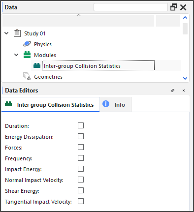
When the Inter-group Collision Statistics Module is enabled, you are able to select the following Properties:
Duration
Energy Dissipation
Forces
Frequency
Impact Energy
Normal Impact Velocity
Shear Energy
Tangential Impact Velocity
In this version of Rocky, you can also choose which particle group (Figure 2) and geometry component (Figure 3) you want to participate in these collections.
Figure 3.19: Additional module options for Particle groups when the Inter-group Collision Statistics module is enabled
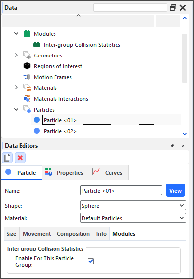
Figure 3.20: Additional module options for a geometry component when the Inter-group Collision Statistics module is enabled
After processing your simulation, specific Curves for the options you enabled will be available for the main Particles entity.
What would you like to do next?
The Inter-particle Collision Statistics module enables the collection of collisions effects upon individual particles resulting from interactions with other particles and boundaries.
Figure 3.21: Options in the Data Editors panel when the Inter-particle Collision Statistics Module is enabled
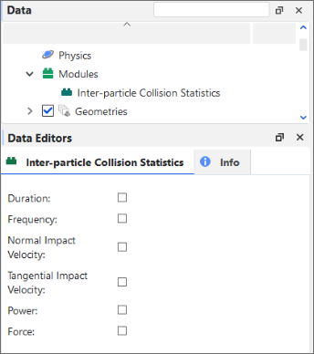
When the Inter-particle Collision Statistics Module is enabled, you are able to select any of the following Properties:
Duration
Force
Frequency
Normal Impact Velocity
Power
Tangential Impact Velocity
After processing your simulation, specific Properties and Curves for the options you enabled will be available for the main Particles entity.
What would you like to do next?
The Intra-particle Collision Statistics module enables the particle-related collision data affecting the surfaces of a Particle set.
Figure 3.22: Options in the Data Editors panel when the Intra-particle Collision Statistics Module is enabled
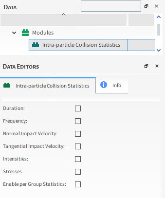
When the Intra-particle Collision Statistics Module is enabled, you are able to select any of the following Properties:
Duration
Frequency
Normal Impact Velocity
Tangential Impact Velocity
Intensities
Stresses
Enable per Group Statistics
After processing your simulation, specific Properties for the options you enabled will be available for each individual Particle set. You can then choose to display this information graphically on the surface of a representative particle in the Particles Details window
What would you like to do next?
The Multibody Dynamics FMU Coupling Module enables you to import FMU files into Rocky without needing to install external Rocky modules into compatible softwares.
Note: For Ansys Motion software and Adams, modules for these software are still needed to export the FMU files.
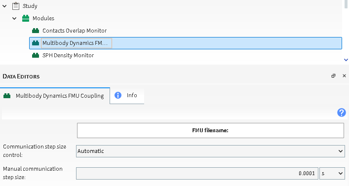
When the Multibody Dynamics FMU Coupling Module is enabled, you are able to import a FMU file through the FMU filename: button, and select the following properties:
Communication step size control: configures the step size method for the communication between Rocky and the FMU file. Three different options can be selected:
Automatic: this method allows Rocky to automatically calculate a communication step size control.
Manual: this method requires a manual input from you. If the manual input value is smaller than Rocky's timestep, it will be overruled by the one calculated by Rocky.
Rocky timestep: this method considers the simulation timestep calculated by Rocky to be the communication step size control.
Manual communication step size: configures the step size of the manual communication method.
Rage: [Positive Values]
Note: This option is only used when the Manual communication step size control is selected.
See Also
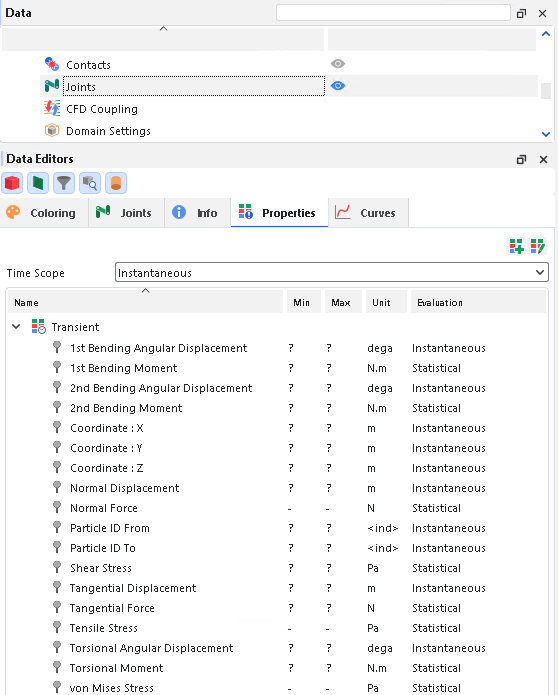
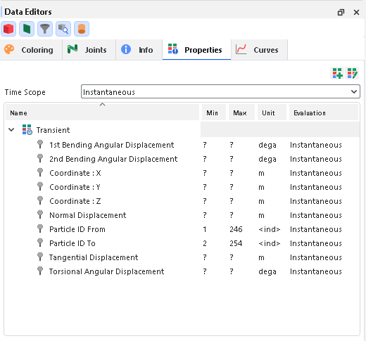
The Joint Statistics module enables new joint properties, with the purpose of generating new statistics data for analysis, such as Stresses and Forces and Torques calculations.
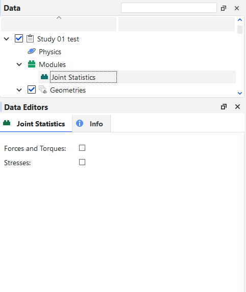
When the Joint Statistics Module is enabled (Figure 1), you are able to select any of the following Properties:
Forces and Torques
Stresses
This way, in the post-processing phase, it is possible to visualize the results of the parameters selected in Joints properties.
See Also
The Particle Instantaneous Energies module enables the collection of energies data related to the velocities and positions of each particle in the simulation. This data can then be used to calculate the kinetic and potential energies of each individual particle, which can be useful when performing global or partial energy balances in a simulation.
Figure 3.26: There are no options in the Data Editors panel when the Particle Instantaneous Energies Module is enabled
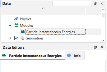
When the Particle Instantaneous Energies Module is enabled, there are no properties or settings to enable.
After processing your simulation, specific Properties for the options you enabled will be available for the main Particles entity.
What would you like to do next?
The Joint Statistics module enables new joint properties, with the purpose of generating new statistics data for analysis, such as Stresses and Forces and Torques calculations.
When the Joint Statistics Module is enabled (Figure 1), you are able to select any of the following Properties:
Forces and Torques
Stresses
This way, in the post-processing phase, it is possible to visualize the results of the parameters selected in Joints properties.
See Also
The Particles Energy Spectra module enables the collection of different kinds of energy statistics per particle type and size category, which can help predict breakage and attrition rates for continuous processes such as grinding mills.
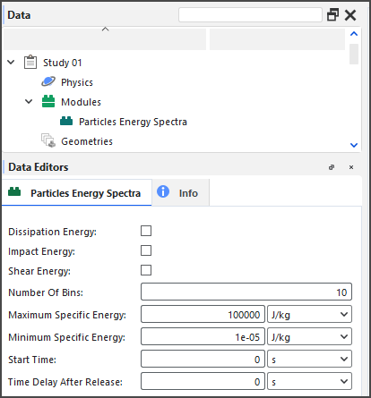
When the Particles Energy Spectra module is enabled (Figure 1), you can choose to collect one or more of three different types of collision energy-Dissipation Energy, Impact Energy, and/or Shear Energy-and define the limits for how the energy data is collected.
In this version of Rocky, you can also choose which particle group (Figure 2) you want to participate in energy spectra collection.
Figure 3.30: Additional module options for Particle groups when the Particles Energy Spectra module is enabled
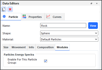
After processing your simulation, you can plot the resulting Cumulative Specific Power curves for the type of energy you collected (Dissipation, Impact, and/or Shear) for each particle set, generated by each size of the particle size distribution, and separated by Specific Energy.
What would you like to do next?
The SPH Mass Flow Rate module is a flow meter that acts by calculating the SPH mass flow rate through a surface, enabling you to choose where you want to measure the mass flow rate.
When the SPH Mass flow Rate Module is enabled (Figure 1), you are able to select one or more surfaces present in the simulation and measure the mass flow rate through them.
Figure 3.32: Geometries options in the Data Editors panel when the SPH Mass Flow Rate Module is enabled
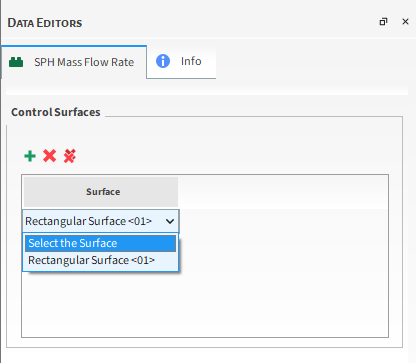
After processing your simulation, specific mass flow rate curves will be available for the surfaces you selected through the module.
What would you like to do next?
The SPH Boundary Interaction Statistics Module enables a collection of SPH boundary-related data, separated into Boundary Properties, where SPH forces are divided into triangles and the nodal force is collected, and Boundary Curves where the collected value refers to the entire geometry.
Figure 3.33: Options in the Data Editors panel when the SPH Boundary Interaction Statistics Module is enabled
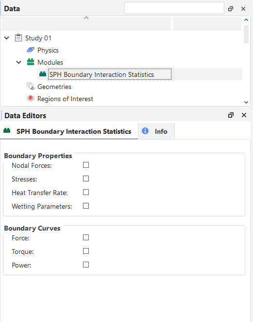
When the SPH Boundary Interaction Statistics Module is enabled (Figure 1), you are able to select any of the following parameters:
Boundary Properties
Nodal Forces
Stresses;
Heat Transfer Rate;
Wetting Parameters.
The Stresses parameter calculates the time average of the stresses on the triangle. If there is no motion and the Cartesian forces are already stored, stresses are calculated with them, otherwise, normal and tangential components of the forces are stored.
The Heat transfer rate parameter calculates the time average of the heat transferred between the fluid and the triangle (positive if the transfer is triangle->fluid, negative otherwise). The Wetting parameters calculates the time average of the ratio between the wet area (approximate) and the triangle area.
Note: Due the use of a kernel function for approximating the wet area, SPH elements located within a distance equal to the kernel radius from a boundary triangle will contribute to that area. This means that if a moving wall approaches an SPH free surface, for instance, it may show wet fractions above zero before actually touching the SPH elements.
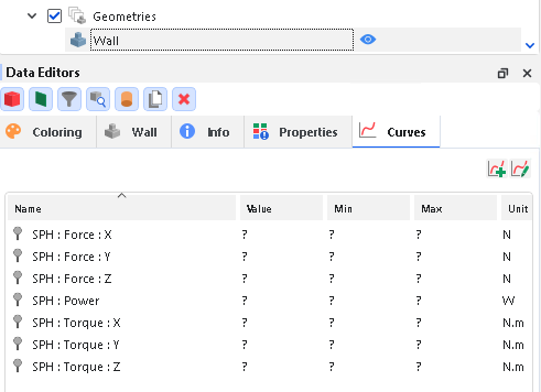
Boundary Curves
Force;
Torque;
Power.
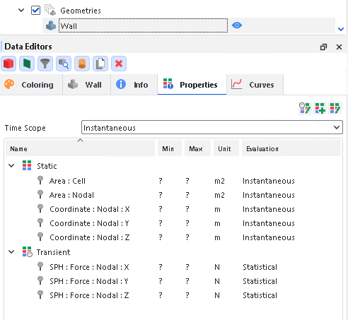
After processing your simulation, specific data based on the options you enabled will be available in Walls Properties or Curves. As you can see in the figures below:
Walls-Properties
Figure 3.34: Results in Walls Properties when the SPH Boundary Interaction Statistics Module is enabled
Walls-Curves
What would you like to do next?
The SPH Density Monitor Module enables the monitoring of density values of the SPH elements during a simulation.
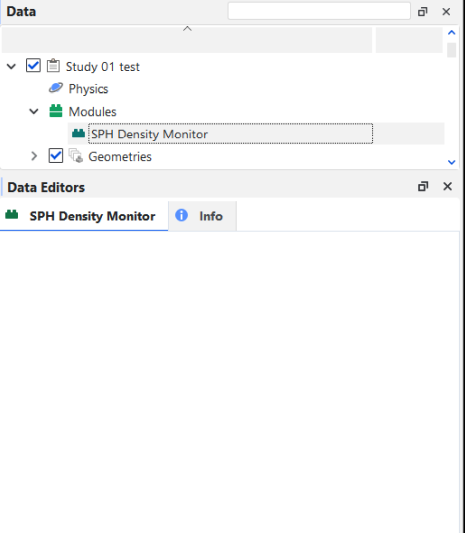
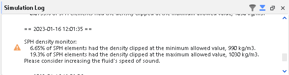
During the simulation, if the module detects that the density values were clipped due the existence of positive or negative deviations that exceeded the maximum allowed values, it will issue a warning, indicating the percentage of SPH elements that had density values clipped. These Warnings are registered in the log file and can be consulted later.
See the example in the figure below:
What would you like to do next?
Learn more Understand Rocky Modules
Learn more About Modules Parameters
The SPH HTC Calculator module calculates the heat transfer coefficient (HTC) through forced convection for each wall triangle. It provides an estimation of heat exchange without requiring a thermal solution.
The heat transfer coefficient is calculated using simple correlations based on local Reynolds and Prandtl numbers. The correlations used for computing the Nusselt number depend on whether the flow is laminar or turbulent, as determined by the user-defined threshold.
Limitations
Listed below are known limitations of the SPH HTC Calculator module:
User input is required for fluid thermal conductivity and specific heat.
The module ignores the internal values of these properties in the fluid material; however, fluid viscosity is still extracted from the fluid material data.
The heat transfer coefficient is computed based on the local Nusselt number, which utilizes the fluid velocity at a specific distance from the wall, as determined by the Distance Factor.
The user has the ability to modify the parameters utilized for calculating the Nusselt number in accordance with the flow characteristics.
Module Options
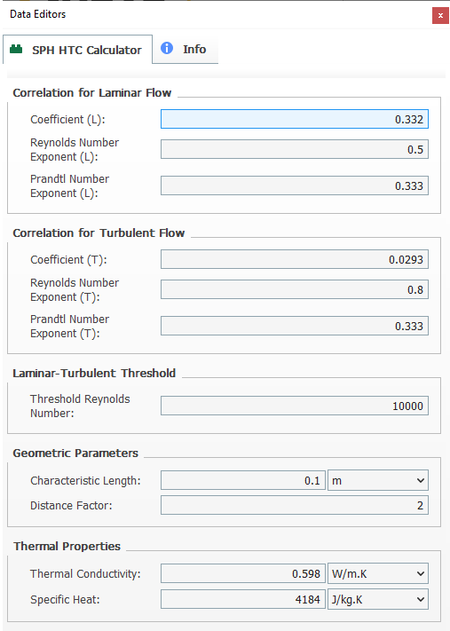
Refer to Figure 3.39: SPH HTC Calculator module options. and the parameter definitions below to understand how to enable and configure the SPH HTC Calculator module. These parameters are explained below:
Coefficient (L): Coefficient used to compute the Nusselt number for a laminar flow. Range: [Positive values]
Reynolds Number Exponent (L): Exponent that raises the Reynolds number to compute the Nusselt number for a laminar flow. Range: [Positive values]
Prandtl Number Exponent (L): Exponent that raises the Prandtl number to compute the Nusselt number for a laminar flow. Range: [Positive values]
Coefficient (T): Coefficient used to compute the Nusselt number for a turbulent flow. Range: [Positive values]
Reynolds Number Exponent (T): Exponent that raises the Reynolds number to compute the Nusselt number for a turbulent flow. Range: [Positive values]
Prandtl Number Exponent (T): Exponent that raises the Prandtl number to compute the Nusselt number for a turbulent flow. Range: [Positive values]
Threshold Reynolds Number: This defines the laminar-turbulent transition. Above this Reynolds number, the flow is considered turbulent. Range: [Positive values]
Characteristic Length: Length used to compute the Reynolds number and the heat transfer coefficient. Range: [Positive values]
Distance Factor: Factor that multiplies the SPH element spacing for computing the distance from the wall at which the velocity is obtained. Range: [Positive values]
Thermal Conductivity: This defines the fluid thermal conductivity, which is used to compute the Prandtl number and the heat transfer coefficient. Range: [Positive values]
Specific Heat: This defines the specific heat used to compute the Prandtl number. Range: [Positive values]
Post-processing abilities
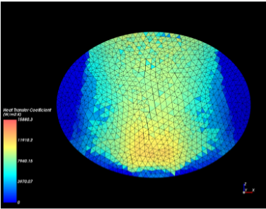
After simulating, a new Heat Transfer Coefficient property becomes available for wall entities. This property aids in visualizing heat exchange between the SPH fluid and each wall.
Figure 3.40: New wall properties are shown in the Data Editors panel when the SPH HTC Calculator module is enabled.
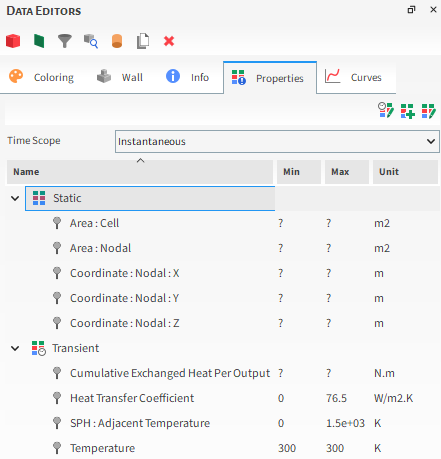
These new properties are explained below:
Heat Transfer Coefficient: This provides the heat transfer coefficient for each wall triangle.
SPH: Adjacent Temperature This provides the SPH adjacent temperature for each wall triangle. When coupling with mechanical this average adjacent temperature is sent to mechanical.
You can analyze these properties in a plot or histogram window. Alternatively, you can graphically display these properties in a 3D View window.
Setting up and using the module
Ensure that the module is enabled. (From the Data panel, select Modules and then from the Data Editors panel, ensure the SPH HTC Calculator checkbox is enabled.)
From the Data panel, under Modules , select the new SPH HTC Calculator entry.
From the Data Editors panel, on the SPH HTC Calculator tab, enter the values you want.
Continue setting up the simulation as you normally would.
Process the simulation as you normally would.
When you are ready to post-process your simulation results, you can make use of the new parameter on the Properties tab for the main Particles entity.
The SPH-DEM Interaction Statistics Module enables the calculation of interaction between particles and fluids within the simulation.
Figure 3.41: Options in the Data Editors panel when the SPH DEM Interaction Statistics Module is enabled
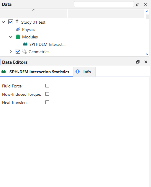
When the SPH-DEM Interaction Statistics Module is enabled (Figure 1), you are able to select any of the following Properties:
Fluid Force
Flow-Induced torque
Heat Transfers
Important: To Heat Transfers option works, it's necessary that the Enable Thermal checkbox in Physics is selected. Otherwise, an error message will appear.
After processing your simulation, specific SPH Properties will appear along with the Particle parameters for the options you enabled before starting your simulation. You can see some of this properties below:
SPH:Flow-Induced Torque
SPH:Flow-Induced Torque: X
SPH:Flow-Induced Torque: Y
SPH:Flow-Induced Torque: Z
SPH:Fluid Force
SPH:Fluid Force: X
SPH:Fluid Force: Y
SPH:Fluid Force: Z
SPH:Heat Transfer Rate
What would you like to do next?
The SPH parameters available define how the simulation of fluid flow is going to be calculated inside Rocky.
Rocky uses an SPH (Smoothed-Particle Hydrodynamics) technique to perform fluid flow simulations. To ensure that the simulation is a good representation of the physics involved, you have control of several parameters that set how the SPH method is going to work in a Rocky simulation. Below you can learn more about these parameters.
Note: Simulation files from previous versions of Rocky that included SPH as a module are not compatible with new versions from 23R1 onwards.
To learn more about how this model is calculated, refer to the SPH Technical Manual. (From the Rocky Help menu, point to Manuals and then click SPH Technical Manual).
Rocky includes an option for thermal modeling in an SPH simulation. To learn more about setting up and using SPH Thermal model in Rocky, refer to the Enable Thermal Modeling Calculations topic.
When setting up an SPH simulation, you have the option of using the Eulerian Solution feature. By default it is enabled. This option allows you to obtain interpolated results for SPH properties (see more About Properties ). This option may result in more use of computational resources. If you want to disable it, you can do so by unchecking the checkbox Eulerian Solution under the SPH item on the data panel). To learn more about setting up and using Eulerian Solution in Rocky, refer to the About SPH Eulerian Solution topic.
The SPH parameters in Rocky can be edited from the SPH entity on the data panel. They are divided into two categories: the SPH Model Parameters with the basic setup needed to perform an SPH simulation, and an Advanced tab, with parameters that allow a fine-tuning of the simulation.
Use the figure and table below to help you understand the various SPH parameters you can set for a simulation project in the SPH Model Parameters tab.
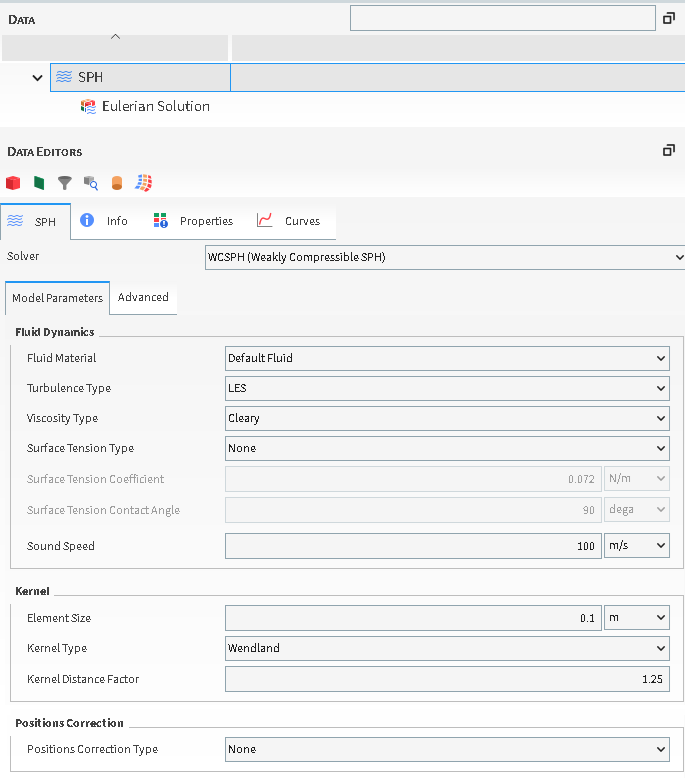
Table 1: SPH Solver Settings
|
Setting |
Description |
|---|---|
|
WCSPH (Weakly Compresible SPH) |
The Weakly Compressible SPH solver is suitable for simulating incompressible fluids, by using an artificial equation of state to compute the relation between pressure and density. |
|
ISPH (Implicit Incompressible SPH) BETA |
The Implicit Incompressible SPH solver is also suitable for simulating incompressible fluids. In this formulation, the fluid incompressibility constraint is enforced by solving a system of linear equations at each simulation time, to compute pressure values that lead to element velocities and displacements that satisfy the constraint. This treatment allows to solve the flow equations with larger timesteps than the ones needed for the Weakly Compressible SPH (WCSPH) formulation. Note: The ISPH can only be used if the Experimental (Beta) Features checkbox is enabled on the Options | Preferences | Additional Features dialog. Important: Note that beta features have not been fully tested and validated. Ansys, Inc. makes no commitment to resolve defects reported against these prototype features. However, your feedback will help us improve the overall quality of the product. We will not guarantee that the projects using this beta feature will run successfully when the feature is finally released so you may, therefore, need to modify the projects. |
|
DFSPH (Divergence-Free SPH) BETA |
The Divergence Free SPH solver is also suitable for simulating incompressible fluids. This solver can be considered an extension of the IISPH formulation, because both enforce a constant density value through the solution of a Poisson pressure equation. However, DFSPH introduces an additional step in which the divergence-free condition is enforced on the velocity field. Note: The DFSPH can only be used if the Experimental (Beta) Features checkbox is enabled on the Options | Preferences | Additional Features dialog. Important: Note that beta features have not been fully tested and validated. Ansys, Inc. makes no commitment to resolve defects reported against these prototype features. However, your feedback will help us improve the overall quality of the product. We will not guarantee that the projects using this beta feature will run successfully when the feature is finally released so you may, therefore, need to modify the projects. |
Note: Simulations with parameters defined in ISPH as a module must be set again, as they will not be compatible with ISPH integrated in the Rocky UI from release 2024 R2 onwards.
Table 2: SPH Model Parameters Tab
Setting | Description | Range |
|---|---|---|
Fluid Dynamics | ||
Fluid Material | Allows you to choose the fluid material that will be used in the simulation. (see also About Modifying Fluid Material Compositions). | Automatically Determined |
Turbulence Type | Defines the turbulence modeling approach.
For additional details about these models, see the SPH Technical Manual. (From the Rocky program Help menu, point to Manuals, and then click SPH Technical Manual.) | Laminar; LES |
Viscosity Type | Defines the viscosity model used in the calculation of SPH element acceleration due viscous forces flow.
For additional details about these models, see the SPH Technical Manual. (From the Rocky program Help menu, point to Manuals, and then click SPH Technical Manual.) Important: It is also important to mention that the Viscosity Type can be overruled by the SPH Turbulent Viscosity Limiter module, which defines a ratio between the set viscosity from the UI and the maximum viscosity that can be achieved. More information about how modules affect simulations can be found at Rocky Simulation Entities that can be Affected by Modules. Also, information about this module can be found in its respective manual. | Cleary; Morris |
Surface Tension Type | Defines the surface tension model used to model free surfaces.
Note: The Pairwise Potential can only be used if the Experimental (Beta) Features checkbox is enabled on the Options | Preferences | Additional Features dialog.
If CSF or Pairwise Potential model are enabled, a new parameter will be required:
Important: When the Pairwise Surface Tension type is selected, the Surface Tension Boundary Angle will be available for the specified geometry, located in the geometry tab (See Imported wall, SPH parameters in the Data Editors panel). | None; CSF; CSS; Pairwise Potential |
Sound Speed / Maximum Expected Velocity | For WCSPH, the Sound Speed, which is about 10x the maximum expected velocity for the simulation must be set here. For IISPH and DFSPH, the value is the Maximum Expected Velocity for the simulation. | Positive Numbers [m/s] |
Kernel | ||
Element Size | Defines the size of an SPH element. For coupled DEM-SPH simulations, an element size at least 3 times smaller than the smallest particle size in the simulation is necessary. | Positive Values |
Kernel Type | Defines the type of kernel function used for SPH calculations
For additional details about these models, see the SPH Technical Manual. (From the Rocky program Help menu, point to Manuals, and then click SPH Technical Manual.) | Cubic; Quintic; Wendland |
Kernel Distance Factor | Defines the kernel distance factor, which affects the size of the kernel support. | Positive Values |
Positions Correction | ||
Positions Correction Type | Defines the formulation applied to prevent SPH elements from clumping together and distribute them more evenly in space.
For additional details about these models, see the SPH Technical Manual. (From the Rocky program Help menu, point to Manuals, and then click SPH Technical Manual.) | None; XSPH; Shift |
Use the figure and table below to help you understand the various SPH parameters you can set for a simulation project in the Advanced tab.

Table 3: SPH Advanced Parameters Tab
Setting | Description | Range |
|---|---|---|
Kernel | ||
Minimum Distance Factor | Defines the factor used to calculate the minimum distance between SPH elements in order to avoid singularities. | Positive Values |
Numerics | ||
User Neighbors List | Allows Rocky to use a neighbors list which is stored in memory. This will speed up the simulation, but if the number of elements in the list exceeds the system memory available, an allocation error may occur. | On or Off |
Timestep Factor | Defines the coefficient used to compute the SPH solver time step. | Positive Values |
Number of Search Cell Sub-Steps | Defines the coefficient that is used to define the search cell size. | Positive Values |
Turbulence Modelling | ||
Cleary Viscosity Factor | Defines the coefficient used in the Cleary formulation of the acceleration due to viscous forces. | Positive Values |
LES Distance Factor | Defines the characteristic length used to compute the turbulent viscosity term. | Positive Values |
LES Smagorinsky Constant | Defines the Smagorinsky constant used to compute the turbulent viscosity term. | Positive Values |
|
Limit Turbulent Viscosity |
The Limit Turbulent Viscosity is used for clipping the viscosity at SPH simulations for turbulent flows. This features aims at preventing the SPH turbulent viscosity from becoming too large and,therefore, possibly destabilizing the simulation. |
On or Off |
|
Maximum Turbulent/Molecular Viscosity Ratio |
This parameter is used for the viscosity clipping, being the maximum viscosity ratio allowed for the current simulation. |
Positive Values |
Positions Correction | ||
Shifting Factor | Defines the shifting factor for the Shift approach. | Positive Values |
XSPH Factor | Defines the XSPH factor used for the XSPH position correction model. | Positive Values |
Free Surface Divergence Limit | Defines the concentration gradient reference used to avoid SPH elements placed near the free surface to be shifted in the normal direction for the Shifting particle correction algorithm. | Positive Values |
Density Correction | Only for WCSPH | |
Update Coupled Density | Defines if the density of the fluid will be updated with the calculations. | On or Off |
Number of Density Correction Steps | Defines the frequency for the density correction calculation. Note: To turn off SPH Density Correction for SPH-only simulations, change the Number of Density Correction Steps to 0. | Positive Values |
Negative Density Deviation | Defines the maximum negative pressure deviation allowed from the initial density value for an SPH element. Note: Another way to turn off SPH Density Correction for SPH-only simulations is to set Negative an Positive Density Deviation to 0. | Positive Values |
Positive Density Deviation | Defines the maximum positive pressure deviation allowed from the initial density value for an SPH element. Note: Another way to turn off SPH Density Correction for SPH-only simulations is to set Negative and Positive Density Deviation to 0. | Positive Values |
Tensile Instability Correction | Only for WCSPH | |
Stability Degree | Defines the degree of the tensile instability correction. | Positive Values |
Stability Negative Factor | Defines the coefficient that multiplies the pressure, if negative, for computing the tensile instability correction term. Default value is zero as the tensile instability correction was found unnecessary for most simulations with the current formulation. | Positive Values |
Stability Positive Factor | Defines the coefficient that multiplies the pressure, if positive, for computing the tensile instability correction term. Default value is zero as the tensile instability correction was found unnecessary for most simulations with the current formulation. | Positive Values |
Wall Boundary Conditions | ||
Boundary Damping Factor | Defines the viscous damping coefficient used in the calculation of the normal force acting on the SPH element due to the wall interaction. | Positive Values |
Boundary Stiffness Factor | Defines the elastic coefficient used in the calculation of the normal force acting on the SPH element due to the wall interaction. | Positive Values |
Boundary Distance Normal Factor | Defines a multiplier used to evaluate the interaction distance between SPH elements and boundaries for the normal force. | Positive Values |
Boundary Distance Tangential Factor | Defines a multiplier used to evaluate the interaction distance between SPH elements and boundaries for the tangential force. | Positive Values |
Surface Tension | ||
Surface Tension Boundary Fraction | Defines a factor used to calculate the surface tension. | Positive Values |
Pressure Calculation | Only for WCSPH | |
Pressure Degree | Coefficient of the equation of state used to compute the relation between pressure and density | Positive Values |
|
Pressure Solution | Only for IISPH and DFSPH | |
| Density Relative Error Tolerance | Defines the tolerance for the relative error in the density calculation. | Positive Values |
| Maximum Number of Iterations | The maximum number of iterations for convergence of the pressure. | Positive Values |
| Pressure Under-Relaxation Factor | Defines a factor introduced to ensure stability of the process, by reducing the amount of changes between iterations. | Positive Values |
| Negative Pressure Factor | Defines the factor that multiplies negative pressures during the iterative solution process. | Positive Values |
What would you like to do?
See Also:
The current SPH feature also has a support for Region of Interest (ROI). This means that it is capable of freezing and disabling SPH-SPH interactions outside a given region. With this feature, there can be a simulation speed increase.
Use the figure below to help you understand the Joints parameters you can set for a simulation project.
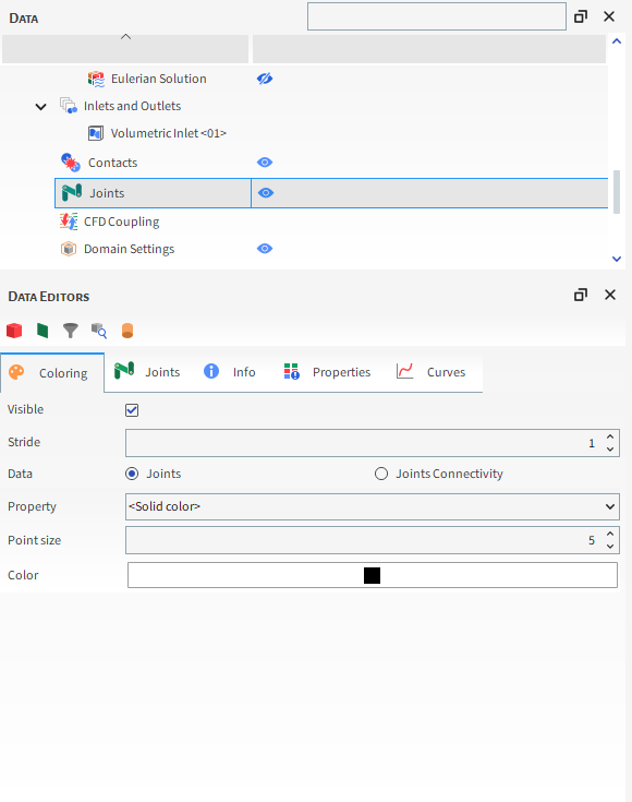
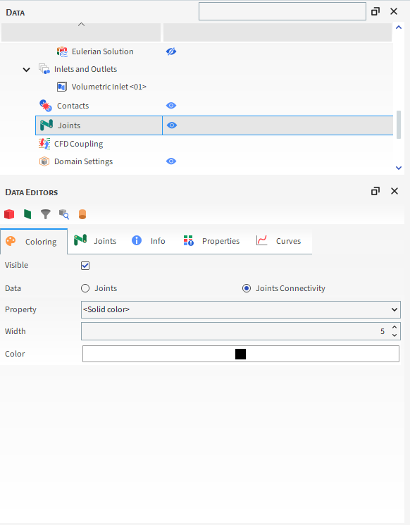
Table 3.1: Joints Parameters - Coloring
|
Setting |
Description |
Range |
|---|---|---|
|
Visible |
When enabled, shows the selected entity in the active view window. |
Turns on or off. |
|
Stride |
One out of this number of data points will be shown when displaying Joints. The lower the number, the more data points will be displayed. |
Whole numbers 1 or greater. |
|
Data |
Joints: Enables the selected joints to be colored in the 3D View. Joints Connectivity:Enables the selected joint connectors to be colored in the 3D View. |
Options limited by the selected Data. |
|
Property |
Provide properties and other color options that apply to the display Data type within which the list is contained.
|
<Solid color>; List of properties automatically generated from the Properties tab. |
|
Point size |
When Joints is selected, this changes the size of the dots used to draw the Joints. |
Positive Values. |
|
Width |
When Joints Connectivity is selected, this changes the thickness of Positive values the lines used to draw the borders. |
Positive Values. |
|
Color |
When Joints or Joints Connectivity are selected and the Property is <Solid Color>, this enables the selected display Data type to be colored in the one solid color chosen. |
Options limited by the selected Color. |
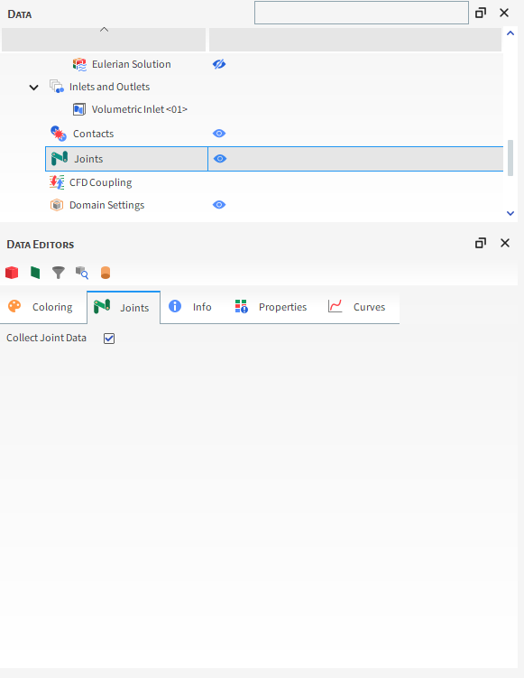
Select Collect Joint Data checkbox for joint data to be collected. This way, after simulation, it's possible to analyze joints positions and displacements in properties tab.
Important: To visualize Joints parameters, it's necessary to clear the Meshed Particles Upscaling checkbox.
What would you like to do?
See Also:
Domain settings enable you to define Coordinate Limits and, if desired, an additional Periodic Domain for your simulation project.
Coordinate Limits determine where in the simulation calculations may occur. This means that any items that fall outside the limits you have defined-including particles and geometries-will not be included in the simulation calculations.
For particles, falling outside the coordinate limits also means they will not be visualized. For particles that are set to be released outside the coordinate limits, this means they will not appear in the simulation at all. For particles that were within the limits but then exited out of them, this means those particles will disappear immediately upon leaving the limits (Figure 1).
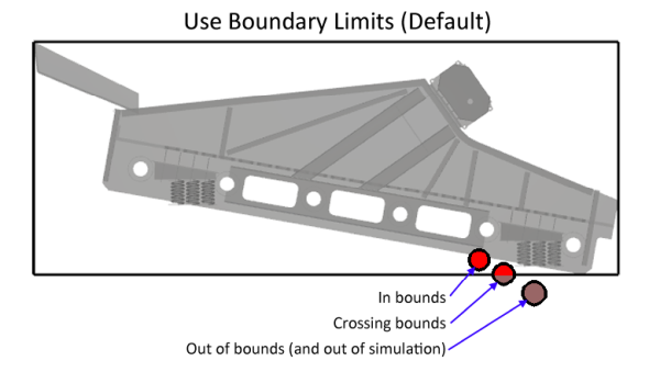
Note: Rocky uses a particle's center point to determine whether it is inside or outside the domain.
For geometries, falling outside the coordinate limits means only that they are not included in calculations. Geometries will still be visualized regardless of whether or not they are within the coordinate limits.
Because of these reasons, it is important that you set your coordinate limits appropriately for the type of simulation you are setting up. For closed systems, such as mixers and mills, where particles are not expected to fall outside of the geometry limits, choosing to use the Use Boundary Limits checkbox might be the best option.
For open systems, such as crushers or vibrating screens, where particles are expected to reach beyond the limits of the geometries, setting your own custom coordinate limits might be a better option.
Tip: To see a walk-through example of setting custom coordinate limits, refer to Tutorial - Vibrating Screen in the Rocky Tutorial Guide.
Periodic Domains enable you to include an additional domain within your simulation Coordinate Limits within which particles that are exiting out one side of the periodic domain area are recycled back into the domain from the opposite side.
In this version of Rocky, periodic domains can either be Cartesian, which are based upon two parallel planes (box-shaped domain), or Cylindrical, which are based upon two intersecting planes rotated by an angle to create a cylindrical sector (wedge-shaped domain).
Both types of periodic domains do not allow the injection of particles outside the bounds of the periodic domain. This means that when setting up your Particle Inputs, ensure that your Continuous Injection Inlet, Volume Fill box bounds, or Custom Input definitions are located well within your periodic domain. (See also About Adding and Editing Particle Inputs.)
Cartesian Periodic Domains are the original type of what used to be known as "periodic boundaries" and whose functionality has been included with Rocky since its earliest releases. When choosing to use Cartesian Periodic Domains, two parallel planes are created along the axis (or combination of axes) you specify. Particles that exit the simulation through one plane will reappear in the simulation through the opposite plane (Figure 2).
Figure 3.49: Particle behavior when exiting only the coordinate limits (left) and then with a periodic cartesian domain set (right)
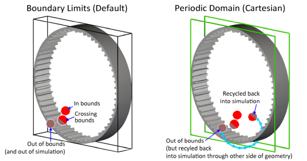
This is especially useful for simulating cross sections or slices of mills; particles flung out of one side of the mill cross section can be recycled back into the simulation from the other side.
Tip: If you choose to set Cartesian periodic domains, ensure that your periodic domain width (the distance between the Min Coordinate and Max Coordinate values) is at least 2.5 times wider than your largest particle size. Or, alternatively, ensure that your largest particle size is less than 0.4 times the width of your periodic domain.
For example, a 0.1 m particle can work in a 0.25 m or wider periodic domain. Alternatively, a 1 m periodic domain can support a 0.4 m or smaller particle size. (See also My particle size is too large for my periodic domain.)
Note: Rocky's Cartesian Periodic Domain functionality was originally designed to be located at the extreme ends of the geometry in question; for example, at the limits of a Mill slice. Sometimes, however, it is desirable to make your periodic domain smaller than the geometry and/or coordinate limits of the domain. Rocky will support you doing this, but be aware that depending on the configuration of the geometries and the periodic limits, it is possible that during the simulation, some particles might go through the walls of your geometries in an unexpected manner. (See also Particles are going through the walls of my geometry.)
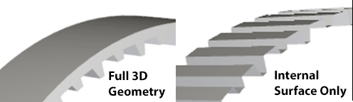
Important: As shown in Figure 3 below, for simulations where the geometry motion is in the periodic plane (i.e., if the periodic direction is Z then the periodic plane is X-Y; if the periodic direction is Y then the periodic plane is X-Z; and if the periodic direction is X then the periodic plane is Y-Z), any triangles whose all 3 vertices exactly lie on the periodic plane should either be removed from the geometry design in a CAD tool prior to being imported into Rocky, or be disabled by Rocky to ensure proper simulation results. In this version of Rocky, these triangles are disabled for you by default. (See also About Solver Parameters.)
Figure 3.50: Geometry triangles lying fully on the periodic plane (in green) should be removed or disabled
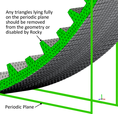
It is recommended that you import only the geometry's internal surface (Figure 4) instead of using the automatic triangle disabling from Rocky. When disabled only, the triangles can be deformed due to wear, and it can cause instabilities in the process — particles could enter into the geometry, for example.
Tip: To see a walk-through example using Cartesian Periodic Domains, refer to the following Workshop:
Similar to Cartesian Periodic Domains, Cylindrical Periodic Domains enable you to specify the locations of two planes between which particles are recycled. But rather than being parallel, the two planes in a Cylindrical Periodic Domain are intersecting and rotated by an angle, creating a cylindrical sector, which can look similar in shape to a "wedge" or "slice" of pie.
This can be useful in cylindrical mixing devices, for example, where simulating only a slice of the device would have similar particle properties as simulating the full device, but with many fewer particles and calculations.
The size of the wedge is determined by the number of (evenly spaced) radial divisions you specify for the cylinder. So a division of 2 would create a wedge half the size of the cylinder; a division of 3 would create a wedge a third the size of the cylinder, and so on.
The placement of the wedge is determined both by the location of the cylinder, which is orientated along the X, Y, or Z Periodic Direction you specify, and the Initial Angle value you specify for the first plane, which will be measured in the positive plane perpendicular to the Periodic Direction.
Tip: The positive angular direction is always counterclockwise when the Periodic Direction is set to point towards outside the screen (top view). This means:
For a Periodic Direction of Y, the Initial Angle is measured from the positive Z axis
For a Periodic Direction of X, the Initial Angle is measured from the positive Y axis
For a Periodic Direction of Z, the Initial Angle is measured from the positive X axis
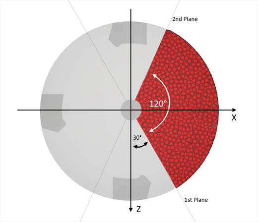
In the mixing drum example shown in Figure 5, the Periodic Direction is Y, the
Initial Angle is 30 degrees, and the Number of Divisions is 3. These settings result
in a periodic, wedge-shaped domain (area in red) that begins 30 degrees counterclockwise in the positive Z direction, and ends 120 degrees (360/3 divisions)
later.
Figure 3.52: Illustration of how the size and location of a Cylindrical Periodic Domain is determined
Limitations and Best Practices
When setting a Cylindrical Periodic Domain, keep in mind the following requirements, limitations, and best practices:
The Periodic Direction must be aligned with one of the three main axes (X, Y, or Z) and must also be parallel to the gravity direction you have set for the simulation.
Because the size of the wedge is determined by how many (evenly spaced) radial divisions you specify, the Number of Divisions value must be a whole integer equal to 2 or greater.
Your Continuous Injection Inlet, Volume Fill box bounds, or Custom Input definitions must be located within the limits of the periodic domain. (See also About Adding and Editing Particle Inputs.)
Using a Particle Trajectory User Process with a Cylindrical Periodic Domain might result in incorrect results. (See also My trajectory lines are outside my periodic domain.)
It is recommended that you design your geometries, define your particle sizes, and set your Cylindrical Periodic Domain limits such that your periodic domain width (the distance between the periodic planes) at any radial distance from the origin is at least 2.5 times wider than your largest particle size. As illustrated on the left side of Figure 6, in most cases, particles at the narrowest part of the wedge will not meet these requirements, which is likely to cause instabilities and affect the accuracy of the results. It is therefore recommended that you apply Cylindrical Periodic Domains only to particles that are simulated in a ring shape, similar to when you specify a Cylinder User Process with the Hole defined (right side of Figure 7).
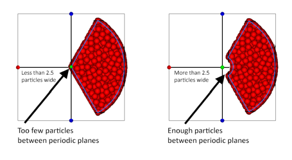 Figure 6: Cylindrical Periodic Domain with full wedge (left) and with center removed (right)
 To reduce the chance of simulation errors, ensure that your geometry triangles fall inside the selected domain and that the periodic planes do not cross the triangle surfaces. The ideal situation is to have the periodic planes crossing along the exact edges of the triangles, as shown on the right side of Figure 6.
 Figure 7: Periodic planes intersecting boundary triangles (left) and aligning on the edges (right)
Use the figures and table below to help you understand the various Domain Settings parameters you can set for a simulation project.
Figure 3.53: Domain Settings, Coordinate Limits parameters in the Data Editors panel (No periodic domain)
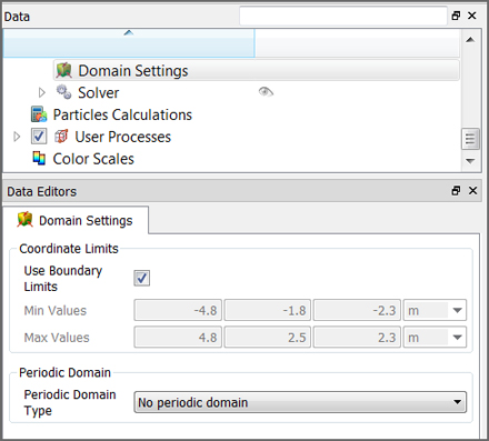

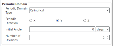
Table 1: Domain Settings parameter options
Setting | Description | Range |
|---|---|---|
Coordinate Limits | ||
Use Boundary Limits | When selected, automatically sets the coordinate limits of the simulation at the extreme ends of the existing geometries. When geometries change or move, the limits will be changed also. Notes:
| Turns on or off |
Min Values | When Use Boundary Limits is cleared, this enables you to set the minimum values for the simulation coordinate limits in the following format: X Y Z These custom limits will be visible in the 3D View. | No limit for X, Y, and Z values but must be lower than Max Values |
Max Values | When Use Boundary Limits is cleared, this enables you to set the maximum values for the simulation coordinate limits in the following format: X Y Z These custom limits will be visible in the 3D View. | No limit for X, Y, and Z values but must be higher than Min Values |
Periodic Domain | ||
Periodic Domain Type | Enables you to choose whether or not to include a periodic domain, and if so, what type of domain you want to include. Specifically:
| No periodic domain; Cartesian; Cylindrical |
Periodic Direction | When either Cartesian or Cylindrical is selected as Periodic Domain Type, this determines the direction periodic domains are enabled. Specifically:
| Turns on or off |
Periodic at Geometry Limits | When Cartesian is set for Periodic Domain Type, enabling this checkbox locates the periodic domain at the farthest edge of the simulation geometries. When cleared, the Min. Coordinate and Max. Coordinate values will be used to define the periodic domain limits. | Turns on or off |
Min Coordinate | Location along the axis specified for Periodic Direction to place the first of two planes that define the box-like shape of the cartesian periodic domain limits. Tip: Ensure the distance from this coordinate to the Max Coordinate is at least 2.5 times wider than the largest particle size. | No limit |
Max Coordinate | Location along the axis specified for Periodic Direction to place the second of two planes that define the box-like shape of the cartesian periodic domain limits. Tip: Ensure the distance from this coordinate to the Min Coordinate is at least 2.5 times wider than the largest particle size. | No limit |
Initial Angle | When Cylindrical is set for Periodic Domain Type, this determines the location of the first of two intersecting planes that define the wedge-like shape of the cylindrical periodic domain limits. How this value is measured depends upon the Periodic Direction specified. Specifically:
Entering a 0 (zero) value will align the first plane with the axis of measure; entering any other value will offset the plane by that angle amount. | No limit |
Number of Divisions | When Cylindrical is set for Periodic Domain Type, this defines how the cylinder will be divided to determine the final size of the wedge. Specifically:
| Whole numbers greater than or equal to 2 |
What would you like to do?
See Also:
Unlike most setup parameters, which you can define only prior to processing, you are able to change the parameters under Execution on the Solver | General tab, or any of the options on the Solver | Advanced tab after processing has started without invalidating your results. You must first Stop processing, change the parameters you want, and then Resume processing again in this scenario. (See also I cannot change my setup parameters during processing.)
Important: In this version of Rocky, Particles Energy Spectra and Contacts Energy Spectra are defined in their own respective modules. (See also About Particles Energy Spectra and About Contacts Energy Spectra.)
Use the figures and tables below to help you understand the various Solver parameters you can set for a simulation project.
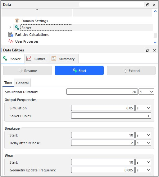
Figure 3.57: Solver | Time parameters for 2-Way Fluent CFD Coupling simulations in the Data Editors panel
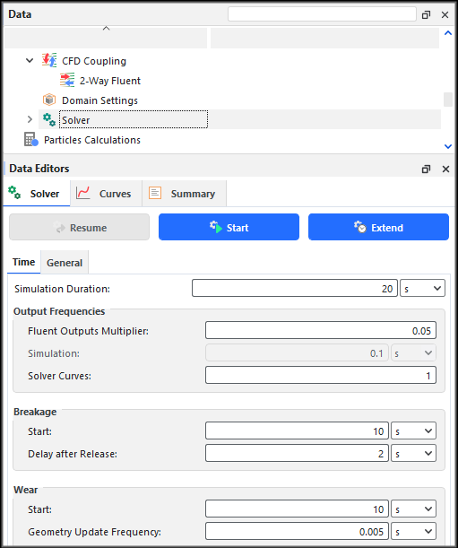
Table 1: Solver | Time parameter options
Setting | Description | Range |
|---|---|---|
Simulation Duration | The total amount of real time that you want the simulation to run. Tip: When calculating the Simulation Duration value, be sure to account for the length and speed of your conveyors, the mass flow rate of your particles, steady-state, and so on. | Positive values |
Output Settings Fluent Outputs Multiplier | For 2-Way Fluent CFD Coupling simulations only, this value determines how many Fluent time steps must occur before simulation files from both Rocky and Fluent are saved. For example, a value of 1 means files will be saved at every Fluent time step; a value of 10 means that files will be saved for every ten Fluent time steps, and so on. (See also About Using the 2-Way Fluent Method.) | Positive, whole values |
Output Settings Simulation | The time intervals at which you want your output files to be saved. Note: This parameter is disabled in 2-Way Fluent CFD Coupling simulations and is instead calculated based upon the Fluent time step and the Fluent Outputs Multiplier. (See also About Using the 2-Way Fluent Method.) Tip: To prevent rotating or vibrating boundaries from appearing like they are moving backwards, divide the rotational velocity (for rotating boundaries) or frequency (for vibrating boundaries) by 2 and then set your simulation output frequency as slightly lower than that value. Tip: Rocky also has a feature to select multiple output frequencies during the simulation, which is useful to increase or reduce the output data after some time, so that specific phenomena can be evaluated with more or less detail. (See also I cannot find the Output Frequency parameter.) | Value must be positive but less than Simulation Duration |
Output Settings Solver Curves | Controls the frequency at which the Solver Curves are updated while the simulation is being processed. The value entered here represents the number of times the Solver Curves will be updated between two consecutive outputs. For example, if the Simulation Output Settings is set to 1 [s] and the Solver Curves Output Frequency is set to 100, it means that the Solver Curves will be updated at every 0.01 [s]. Note: Rocky will limit the time interval for updating the Solver Curves Frequency to be larger than 100 simulation time steps. | Whole values greater than zero |
Breakage Start | The amount of time you want to wait before starting to calculate particle breakage. Tip: It is best practice to set your Breakage Start time to begin after a steady state has been reached in your particle flow. | Value must be positive but less than Simulation Duration |
Breakage Delay after Release | The amount of time you want to wait after a particle has been released before starting to calculate particle breakage. | Value must be positive but less than Simulation Duration |
Wear Start | The amount of time you want to wait before starting to calculate belt and boundary wear. Tip: It is best practice to set your Wear Start time to begin after a steady state has been reached in your particle flow. | Value must be positive but less than Simulation Duration |
Wear Geometry Update Frequency | Amount of time between wear geometry updates. A smaller value will produce smoother transitions between updates but might increase processing time; a larger value will produce rougher transitions between updates, but will take less time to process. (See also See Surface Wear on the Geometry Itself.) | Positive |
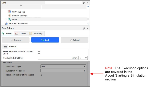
Table 2: Solver | General parameter options
Setting | Description | Range |
|---|---|---|
Release Particles without Overlap Check | For Continuous Injection Inputs only, when enabled, this overrides the setting that delays particles from discharging from an inlet if other particles or boundaries are in the way. When cleared, Rocky will delay releasing any overlapped particles by the Overlap Particles Delay time provided. WARNING: Selecting this item with large particles or high particle velocities could cause problems with your simulation and might result in Rocky hanging or shutting down. Tip: Rather than releasing particles without checking for overlaps (i.e., enabling this checkbox), it is recommended that you instead increase the duration between your input's Start Time and Stop Time settings (see also About Adding and Editing Particle Inputs) and/or increase the size of your inlet geometry to allow more space and time for your particles to be released. | Turns on or off |
Overlap Particles Delay | When the Release Particles without Overlap Check checkbox is cleared, this defines the amount of time Rocky will wait to release a particle from an inlet should it determine that other particles or boundaries are in the way. | Positive values |
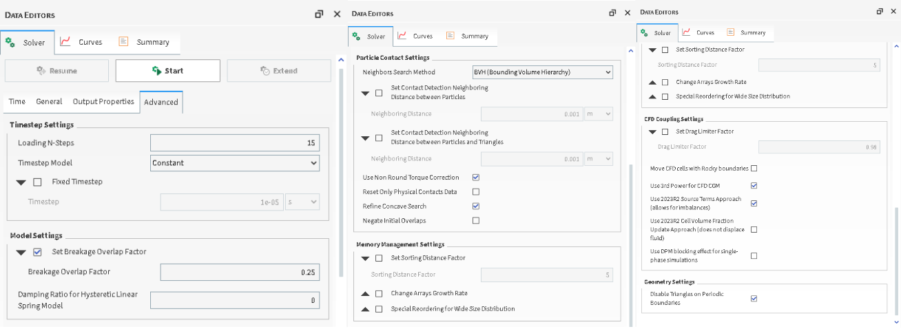
Note: The Advanced tab only appears when the Advanced Features checkbox is enabled on the Additional Features tab of the Options | Preferences dialog. (See also About Setting Global Preferences.)
Table 3: Solver | Advanced tab (Advanced Features) settings
Setting | Description | Range |
|---|---|---|
Timestep Settings Loading N-Steps | Value used to calculate timesteps. In general, the lower the value, the faster the processing but the more unstable the results. Higher values (for example, above 15) are recommended if you are interested in collecting energy spectra or calculating breakage. | Positive values Recommended: 10-30 |
Timestep Settings Timestep Model | Determines how Rocky treats the calculation of an overlap in cases when a specific collision would allow for a bigger timestep than the one defined for the simulation. Important: What you set for Timestep Model does not change the timestep itself, only whether overlaps are calculated always with Rocky's normal, full procedure (Constant) or, whenever possible, with a simplified one (Variable). Specifically:
| Constant; Variable |
Timestep Settings Fixed Timestep | When enabled, it allows you to define an initial value for the Timestep Duration, which is shown on the Simulation Summary screen. (See also About the Simulation Summary.) When cleared, Rocky will automatically calculate this value based upon particle size, density, elastic properties, and so on. Useful only when you want to override the Rocky value, which could lead to faster processing but could also decrease stability. | Turns on or off |
Timestep Settings Timestep | When Fixed Timestep is enabled, this sets a value for Timestep Duration that will override the value Rocky typically calculates automatically based upon several different factors. (See also About the Simulation Summary.) | Positive values |
Model Settings Set Breakage Overlap Factor | When enabled, it allows you to define a factor for particle breakage overlap as a fraction of Minimum Size (see also About Adding and Editing Particle Sets) of the breakage fragment, which affects how easily particles break when coming into contact with boundaries. When enabled, a particle will break when the Breakage Overlap Factor with the boundary it comes into contact with is reached-regardless of the particle's actual strength. The fragment size distribution for this breakage will be defined by the energy of the particle's contact at the time of breakage. Note: This overlap factor is enabled automatically by Rocky when Experimental Features (see also About Setting Global Preferences) is turned off. Turning on Experimental Features allows you the ability to change or disable the overlap factor value. When cleared, a contacting particle will break only when its energy strength is reached, thus creating a possibility of the fragments being generated on the other side of a boundary if the overlap on breakage is high enough for that. Enabling this parameter can be useful when you want to avoid fragment generation on the other side of a boundary. This can occur when particles that have large boundary overlaps due to low contact stiffness, break and the fragments in the overlap area end up on the wrong side of the boundary. It can also, however, introduce errors in particle strength distribution. | Turns on or off |
Model Settings Breakage Overlap Factor | When Set Breakage Overlap Factor is enabled, a particle will break when its overlap with the contacting boundary reaches the value of this factor multiplied by the Minimum Size (see also About Adding and Editing Particle Sets) of the fragment-even if the current energy is not enough for the particle to break. | Positive values |
Model Settings Damping Ratio for Hysteretic Linear Spring Model | Enables you to specify the value of the damping ratio, The damping force in the hysteretic model is only activated during long-term contacts with the singular purpose of eliminating spurious low-amplitude oscillations in the overlap that usually arises in those cases. See also the Rocky DEM Technical manual. (From the Help menu, point to Manuals and then click DEM Technical Manual.) | 0-1 |
Particle Contact Settings Neighbors Search Method | Enables you to specify the method that the solver uses to search neighboring particles. This affects the efficiency and consequently the time and computational resources required to complete a simulation. Each method is best suited for a specific situation. BVH (Bounding Volume Hierarchy): method best suited for higher PSD and high aspect ratio particles. Regular Grid (Performance Enhanced): method best suited for lower PSD and spherical particles. Its focus is on performance, so it may require more computational resources (ex.: system memory). Regular Grid (Memory saving): method best suited for lower PSD and spherical particles. Its focus is on saving computational resources. This computational resources. It allows for cases with more particles to be evaluated, at the expense of the time required to perform the simulation. | BVH (Bounding Volume Hierarchy); Regular Grid (Performance Enhanced); Regular Grid (Memory Saving) |
Particle Contact Settings Set Contact Detection Neighboring Distance between Particles | When enabled, it allows you to manually set the distance away from a particle that defines the boundary within which neighboring particles are considered for contact. When cleared, this distance is automatically calculated by Rocky. | Turns on or off |
Particle Contact Settings Neighboring Distance | When Set Contact Detection Neighboring Distance between Particles is enabled, this value overwrites the distance that is automatically calculated by Rocky. | Positive values |
Particle Contact Settings Set Contact Detection Neighboring Distance between Particles and Triangles | When enabled, it allows you to manually set the distance away from a particle that defines the boundary within which neighboring triangles are considered for contact. When cleared, this distance is automatically calculated by Rocky. | Turns on or off |
Particle Contact Settings Neighboring Distance | When Set Contact Detection Neighboring Distance between Particles and Triangles is enabled, this value overwrites the distance that is automatically calculated by Rocky. | Positive values |
Particle Contact Settings Use Non Round Torque Correction | When enabled for shaped particles, this improves the contact overlap algorithm by increasing the accuracy of the contact point position calculations and thus increasing the accuracy of the rotational calculations for shaped particles. Notes:
| Turns on or off |
Particle Contact Settings Reset Only Physical Contacts Data | When enabled for shaped particles, the contact parameters during contact detection will be reset from existing ones for physical contact only. When cleared, both near contacts and physical contacts will result in a reset. Enabling this setting will lead to slower calculations but will save memory, which might be important for GPU simulations in particular. | Turns on or off |
Particle Contact Settings Refine Concave Search | When enabled, Rocky performs a second, more refined search for neighboring particles in addition to the standard search that is done by default. This second search is specifically designed for concave shapes, and serves to provide a more accurate near-neighbors list by removing particles from the initial results that are not actually near neighbors. Reducing the results for concave shapes saves memory and may also save computational time due to fewer possibilities for contacts needing to be considered. For convex shapes processed on GPUs, however, this may slow down processing so it is recommended that this be enabled only for concave shapes. When cleared, only the standard search method is used. | Turns on or off |
Particle Contact Settings Negate Initial Overlaps | Especially for projects in which some particles are enabled only after a certain condition is met (distance, temperature, time, etc.), this feature can help you avoid unrealistic forces due to a just-enabled particle landing inside the boundaries of another particle. When enabled, Rocky negates—for only the first collision a particle experiences— the first overlaps. This means that when a particle is enabled later into the simulation and happens to land within the boundaries of another particle, those initial overlaps will not be computed. It is only on the subsequent overlaps that contact forces detection will start. When cleared, overlaps are always considered in forces calculations. Notes:
| Turns on or off |
Memory Management Settings Set Sorting Distance Factor | When enabled, allows you to control how frequently particle data stored in memory is reordered in a sorting operation. (This operation happens on both CPU and GPU). Sorting helps guarantee that data from a particle is stored in memory near the data from neighboring particles in the 3D space, which can help with performance. The sorting distance itself is defined in Rocky as the average distance between neighbor particles times the Sorting Distance Factor, the latter of which this parameter enables. During the simulation, whenever a particle moves a distance larger than or equal to the sorting distance since the last sorting, a new sorting operation is triggered for all active particles at that time. Since sorting can be relatively expensive in terms of computation time, an adequate sorting frequency may be crucial for improving performance in cases where particles are moving at high velocities. When cleared, the sorting distance calculated by Rocky is used. | Turns on or off |
Memory Management Settings Sorting Distance Factor | When Set Sorting Distance Factor is enabled, this value is multiplied by the average distance between neighbor particles calculated by Rocky. The larger the value of this factor, the less frequent the sorting. | Positive values |
Memory Management Settings Change Arrays Growth Rate | When enabled, it allows you to change the rate of growth for the internal memory arrays used during simulation processing. When cleared, the default value of 1.0 will be used. | Turns on or off |
Memory Management Settings Arrays Growth Rate | When Change Arrays Growth Rate is enabled, this allows you to change the rate of growth for the internal memory arrays used during simulation processing. | Positive values |
Memory Management Settings Special Reordering for Wide Size Distribution | When enabled, bigger particles are moved to the end of the internal memory array used to store them during processing. This reordering can be especially useful in cases with big differences in particle sizes (size ratios ~ 100 for instance), which can sometimes cause memory issues during processing. When cleared, only the standard order is used. | Turns on or off |
Memory Management Settings Particle Size Limit for Reordering | When Special Reordering for Wide Size Distribution is enabled, this defines the minimum size of the "bigger" particles in the simulation that will be reordered. | Positive values Note: This value must be smaller than the size of the biggest particle in the simulation |
CFD Coupling Settings Set Drag Limiter Factor | When enabled, it allows you to limit the effects of drag upon the particles that are affected by fluid interactions. When cleared, Rocky uses the full force of the Drag Law that is set. (See also About Using the 1-Way Fluent Method and About Using the 2-Way Fluent Method.) | Turns on or off |
|
CFD Coupling SettingsMove CFD Cells with Rocky Boundaries |
It uses motion properties in order to rotate the fluid mesh inside Rocky, so that both CFD domain and Rocky boundaries are always syncronized. This allows the use of larger CFD timesteps, resulting in improved performance and a stable solution. When enabled it seamlessly synchronizes the movement of the Fluent CFD mesh with the corresponding movement of the Rocky boundaries, ensuring smooth coordination between them. Note: This feature is available only for 2-way CFD coupled simulations with moving meshes. |
Turns on or off |
CFD Coupling Settings Drag Limiter Factor | When Set Drag Limiter Factor is enabled, the drag applied to
the particles is limited by this value,
Setting values below 1 increases the stability of integration for very small particles with large velocities relative to the fluid. However, it also decreases the accuracy of drag force calculations. | Positive values |
|
CFD Coupling Settings Use 3rd Power for CFD CGM | When it is enabled the forces will be corrected by a third power factor instead of the default second power. | Turns on or off |
|
CFD Coupling Settings Use 2023 R2 Source Terms Approach (allows for imbalances) | When it is enabled the 2023 R2 Source Terms Approach will be used in 2-Way couplings simulations, allowing for imbalances. | Turns on or off |
|
CFD Coupling Settings Use 2023 R2 Cell Volume Fraction Update Approach (does not displace fluid) | When it is enabled the 2023 R2 Cell Volume Fraction Update Approach will be used. | Turns on or off |
|
CFD Coupling Settings Use DPM blocking effect for single phase simulations | When it is enabled the DPM blocking effect will be considered for 2-Way single phase simulations. | Turns on or off |
Geometry Settings Disable Triangles on Periodic Boundaries | When enabled for simulations using Cartesian Periodic Domains (see also About Domain Settings Parameters), this option disables from calculations (but keeps in visualizations) any geometry triangles whose all 3 vertices land exactly on the periodic domain. Because of the way periodic domains work, it is best practice to remove these triangles when initially designing your geometry in a CAD tool. This option ensures that if any of these triangles do appear in your simulation, they will not negatively affect your calculations. When cleared, any geometry triangles whose all 3 vertices land exactly on the periodic domain will be allowed to participate in the simulation. This could result in incorrect particle contacts with these triangles which, especially for simulations with surface wear modification (see Enable and View Surface Wear Modification on an Imported Geometry), could result in inaccurate wear patterns. Enabling this setting might therefore be particularly important when simulating liners and lifters within SAG or HPGR mill slices. | Turns on or off |


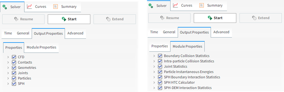
|
Output Properties |
Description |
Range | |
|---|---|---|---|
| Properties | Particles | Select all particle properties that can be used in the post-processing |
Turns on or off |
|
SPH |
Select all SPH properties that can be used in the post-processing |
Turns on or off | |
| Geometries |
Select all Geometries properties that can be used in the post-processing |
Turns on or off | |
|
CFD |
Select all CFD properties that can be used in the post-processing |
Turns on or off | |
|
Joints |
Select all Joints properties that can be used in the post-processing |
Turns on or off | |
|
Contacts |
Select all Contacts properties that can be used in the post-processing |
Turns on or off | |
| Module Properties | Boundary Collision Statistics | Select all Boundary Collision Statistics properties that can be used in the post-processing |
Turns on or off |
|
Intra-particle Collision Statistics |
Select all Intra-particle Collision Statistics properties that can be used in the post-processing |
Turns on or off | |
| Joints Statistics |
Select all Joints Statistics properties that can be used in the post-processing |
Turns on or off | |
|
Particle Instantaneous Energies |
Select all Particle Instantaneous Energies properties that can be used in the post-processing |
Turns on or off | |
|
SPH Boundary Interaction Statistics |
Select all SPH Boundary Interaction Statistics properties that can be used in the post-processing |
Turns on or off | |
|
SPH HTC Calculator |
Select all SPH HTC Calculator properties that can be used in the post-processing |
Turns on or off | |
|
SPH-DEM Interaction Statistics |
Select all SPH-DEM Interaction Statistics properties that can be used in the post-processing |
Turns on or off | |
What would you like to do?
See Also:
From the Data panel, select in turn each of the items listed below and then in the Data Editors panel for each item, make the selections and/or enter the values you want:
The top-most "Study" item
Physics
Modules
Domain Settings
Solver (including all three of the Time, General, and Energy Spectra tabs)
See Also:
Geometries are the physical boundaries that make up the components that are going to be simulated in Rocky. They can be default geometries which are included within Rocky and also geometries that you import from various CAD programs, or from Ansys Fluent or Ansys Motion setup files.
You can add as many individual geometry components as you want to your simulation in any combination you desire.
However, if you are using a particle or fluid inlet to release DEM particles or SPH elements into your simulation (see also About Adding and Editing Inlets and Outlets), before you are able to process the simulation, you must have a minimum of at least one inlet set up. If you are using a Volumetric Inlet, a simulation can be set up with no geometries in it.
Once you add the geometries you want, you can then change the parameters to achieve the behavior you want. The parameters you change can include the size, shape, and behavior of the default geometries included within Rocky, or special movements of the geometries you have imported, such as gates that lift or turn, for example.
At any point, you can see how your geometries look in a 3D View (see also Create and Modify a 3D View).
What would you like to do?
See Also:
There are two categories of geometries that you can add to your simulation: surfaces and walls; additionally Rocky offers you the option to use templates that can combine both types of geometries.
Tip: Surfaces have a Normal Direction property, which indicates the direction of injection and removal for inlets and outlets and, also, the sign of flow measurements. In Rocky, there is an Invert Normal option, which inverts the normal o the surface and, as a consequence, inverts the directions for inlets/outlets and the flow measurements.
Surfaces are geometries that allow for the passage of SPH elements or DEM particles. They can be set up as inlets, outlets, or as flow measuring surfaces. They can also delimit regions in space that can be filled with fluid or particles. If you want a geometry to act as an barrier that can stop fluid or particles from flowing through it, this geometry must be set up as a wall.
IMPORTANT: If you want to use a surface as an Inlet or an Outlet, the surface must be planar (i.e. it should be contained into a single plane).
In Rocky geometries can be created or imported from external CAD/CAE softwares. The following options to create or import geometries are available (through the Geometry option on the Data panel) (see the image below):
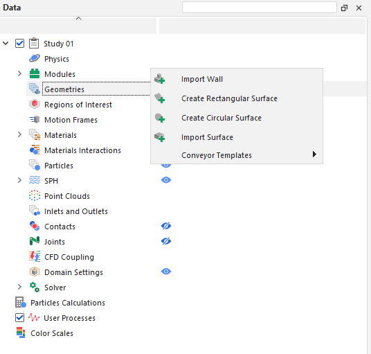
Import Wall: allows you to import a geometry (see also Import Wall or Surface Geometries) that will act as a Wall.
Create Rectangular Surface: allows you to create a rectangular geometry inside Rocky (see also Add New Circular and Rectangular Surfaces) that will act as a Surface.
Create Circular Surface: allows you to create a circular geometry inside Rocky (see also Add New Circular and Rectangular Surfaces) that will act as a Surface.
Import Surface: allows you to import a geometry (see also Import Wall or Surface Geometries) that will act as a Surface.
Conveyor Templates: allows you to create templates of feeding or receiving conveyors (see also Add a Conveyor Template). These templates contain all the necessary Walls and Surfaces.
In addition to the possibility to import Walls or Surfaces into your project, you can also convert Walls into Surfaces and Surfaces into Walls.
To do so, right-click the choose geometry, in the Data Panel, and then go to the option Convert to, as illustrated in the Figures below:
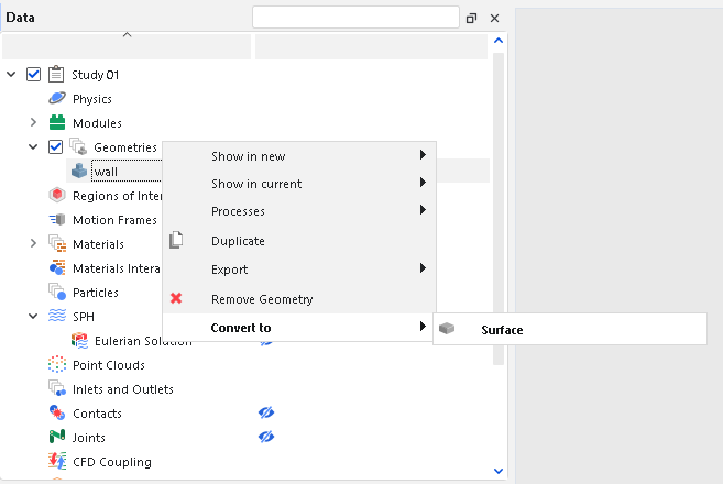
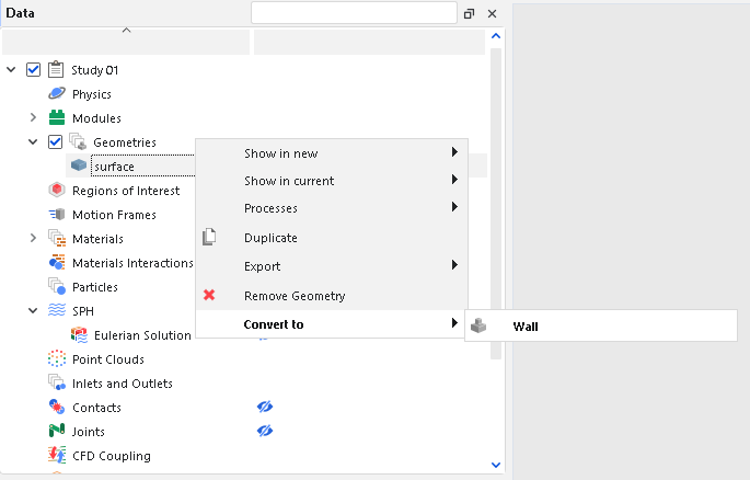
What would you like to do?
You can create rectangular and circular planar surfaces inside Rocky, eliminating the need of importing these geometries from an external CAD software. Since these geometries will act as an surface, you can use them to set inlets, outlets (see also Add and Edit Inlets and Outlets) and to perform flow measurements.
To create these surfaces, do all of the following:
From the Data panel, click Geometries, and then from the Data Editors panel, click the Create Rectangular Surface or Create Circular Surface button. A new Rectangular/Circular Surface component appears under Geometries in the Data panel. Tip: You may also access this functionality from the right-click menu on the Data panel.
From the Data panel, click the Rectangular/Circular component you just added and then from the Data Editors panel, on the main Rectangular/Circular Surface tab, enter the Name you want. You can also edit the properties listed in the table below.
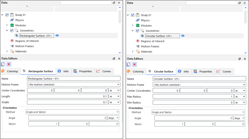
Table 1: Options available when creating a rectangular or circular surface
Setting | Description | Range |
|---|---|---|
Name | Enables you to specify a unique identifier for the geometry component | 99 character limit |
Motion Frame | Enables you to select which Motion Frame you want assigned to the geometry. (See also About Creating and Applying Motion Frames.) | Automatically provided |
Center Coordinates | Enables you to define X, Y and Z coordinates of the center of the geometry. | Any value |
Max Radius (Circular Surface Only) | Defines the radius of external limit of the circular geometry. | Positive Values |
Min Radius (Circular Surface Only) | Defines the radius of internal limit of the circular geometry. | Positive Values |
Lenght (Rectangular Surface Only) | Defines the transverse dimension of the rectangular geometry. | Positive Values |
Width (Rectangular Surface Only) | Defines the longitudinal dimension of the rectangular geometry. | Positive Values |
Method | Enables you to select how you want to define the orientation of the geometry. Specifically:
| Angles; Angle and Vector; Basis Vectors |
Method Angles | ||
Order | When Angles is selected for Orientation, this defines the order in which the three Rotation fields will be applied. | XYZ; ZXY; YXZ; YZX; ZXY; ZYX |
Local Angles | When Angles is selected for Orientation, this defines what coordinate system will be used as a basis for the angle specified. Specifically:
| Turns on or off |
Rotation | When Angles is selected for Orientation, this is the degree of cube rotation in each of the three directions specified by the Order provided. | Any value |
Method Angle and Vector | ||
Angle | When Angle and Vector is selected for Orientation, this is the angle the cube will rotate around the Vector defined. | Any value |
Vector | When Angle and Vector is selected for Orientation, this is the X, Y, and Z components that define the vector around which the cube will rotate, using the Angle defined. | No limit but the values entered will be normalized |
Method Basis Vectors | ||
X direction | When Basis Vectors is selected for Orientation, this is the coordinate values defining the first of three directional vectors that together define the final orientation of the cube. Tip: To ensure correct results, make sure you define this vector as orthogonal (perpendicular) to the other two vectors. | No limit but the values entered will be normalized |
Y direction | When Basis Vectors is selected for Orientation, this is the coordinate values defining the second of three directional vectors that together define the final orientation of the cube. Tip: To ensure correct results, make sure you define this vector as orthogonal (perpendicular) to the other two vectors. | No limit but the values entered will be normalized |
Z direction | When Basis Vectors is selected for Orientation, this is the coordinate values defining the third of three directional vectors that together define the final orientation of the cube. Tip: To ensure correct results, make sure you define this vector as orthogonal (perpendicular) to the other two vectors. | No limit but the values entered will be normalized |
What would you like to do?
Learn more Add a Conveyor Template
Learn more About Adding and Editing Inlets and Outlets
See Also:
All geometries that are not rectangular or circular, or have a template inside Rocky (such as conveyors), need to be imported. Imported geometries can be set up as both wall and surface. When imported as surfaces, the geometry can be used for flow measurements, as an inlet or an outlet (if planar). Importing geometry as walls allows for them to be used for additional calculations (such as surface wear or heat conduction).
Rocky supports importing geometries with the following file extensions: STL, DXF, XGL, CAS, CAS.GZ, CAS.H5, MSH, FMU, or DFG.
To import these surfaces, do all of the following:
From the Data panel, click Geometries, and then from the Data Editors panel, click the Import Wall or Import Surface button. Tip:You may also access this functionality from the right-click menu on the Data panel.
Select the file that you want to import into Rocky and click Open. Tip:To save time on larger projects, you may also want to import multiple components at once by multi-selecting several files on the Select file to import dialog.
Select the file that you want to import into Rocky and click Open
After choosing which file(s) you want to import, you are asked to define several options that enable you to determine the scale and unit of the imported file(s) (Figure 1). In addition, you can either choose to import the component names as they are by leaving the Prefix for imported Geometries blank, or you can add custom text to prefix the component name with whatever you like.
Imported geometry components may be replaced with a different geometry file prior to processing. (See also Replace an Imported Geometry File.) Note: If you want to use a geometry for flow measurements or other post-processing analysis, it must be imported into Rocky before the simulation has started. In post-processing Rocky is not able to import a geometry without needing to restart the simulation.
Use the figure and table below to understand the various import parameters you can set for your imported geometries and then use the procedures that follow to learn about how to add geometry components to your simulation setup.
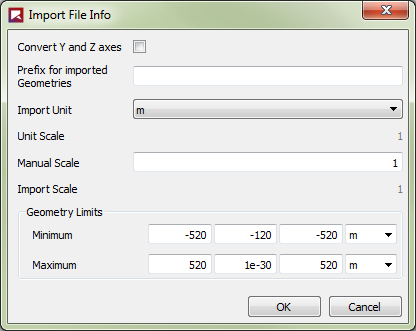
Table 1: Import options displayed in the Rocky dialog
Setting | Description | Range |
|---|---|---|
Convert Y and Z axes | Selecting this option will change the axis of the imported geometry. | Turns on or off |
Prefix for imported Geometries | When cleared (blank), the name of the imported file will be displayed in the Geometries list. When defined, this additional name will be displayed directly before the imported name in the Geometries list. If the geometry contains multiple components, each component will have this same prefix followed by the (unique) imported name of the file. | 99 character limit |
Import Unit | Enables you to change the units of the imported geometry. | Various units of length |
Unit Scale | Displays the unit scale based upon the Import Unit set. For example, if Import Unit is left as the default value, the Unit Scale will be 1. | Automatically determined |
Manual Scale | Enables you to manually adjust the scale by any factor you want. Leaving the value at 1 will have no additional affect upon the scale. | All values |
Import Scale | Displays the final import scale based upon the Manual Scale and Import Unit values set. For example, if both those options are left as the default values, the Import Scale will be 1. | Automatically determined |
Geometry Limits | ||
Minimum | The coordinates (in X Y Z format) of the lowest points geometry triangles are drawn. | No limit |
Maximum | The coordinates (in X Y Z format) of the highest points geometry triangles are drawn. | No limit |
Important: If an STL file is loaded and a triangle is missing, it might be because the triangle has an area equal to zero (two or three vertices at the same position). Rocky automatically deletes triangles with this characteristic to avoid issues with the simulation. If this occurs, check the coordinates of the missing triangles and ensure that none are coincident.
Use the figure and table below to understand the various import parameters you can set for a geometry that was imported as a surface.
Prior to processing, Geometry components may be replaced with a different geometry file, (see also Replace an Imported Geometry File), and have a Motion Frame assigned to them (see also Apply a Motion Frame to an Imported Geometry.)
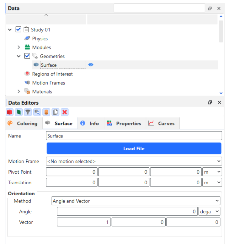
Table 2: Options available for geometries imported as surfaces
Setting | Description | Range |
|---|---|---|
Name | Enables you to specify a unique identifier for the geometry component | 99 character limit |
Motion Frame | Enables you to select which Motion Frame you want assigned to the geometry. (See also About Creating and Applying Motion Frames.) | Automatically provided |
Pivot Point | The coordinate location of the point around which the surface will pivot, as specified in the X, Y, and Z directions. Note: In the calculation order, the rotation is calculated before the translation. In this way, the Pivot Point presented in the UI does not include the translation values, therefore to obtain the real value, it is necessary to sum the pivot point values with the translation values. | No limit |
Translation | Enables you to move the geometry in the X, Y and Z directions | Zero or Positive Values |
Orientation | Enables you to select how you want to define the orientation of the geometry. Specifically:
| Angles; Angle and Vector; Basis Vectors |
Orientation Angles | ||
Order | When Angles is selected for Orientation, this defines the order in which the three Rotation text fields will be applied. | XYZ; ZXY; YXZ; YZX; ZXY; ZYX |
Local Angles | When Angles is selected for Orientation, this defines what coordinate system will be used as a basis for the angle specified. Specifically:
| Turns on or off |
Rotation | When Angles is selected for Orientation, this is the degree of cube rotation in each of the three directions specified by the Order provided. | Any value |
Orientation Angle and Vector | ||
Angle | When Angle and Vector is selected for Orientation, this is the angle the cube will rotate around the Vector defined. | Any value |
Vector | When Angle and Vector is selected for Orientation, this is the X, Y, and Z components that define the vector around which the cube will rotate, using the Angle defined. | No limit but the values entered will be normalized |
Orientation Basis Vectors | ||
X direction | When Basis Vectors is selected for Orientation, this is the coordinate values defining the first of three directional vectors that together define the final orientation of the cube. Tip: To ensure correct results, make sure you define this vector as orthogonal (perpendicular) to the other two vectors. | No limit but the values entered will be normalized |
Y direction | When Basis Vectors is selected for Orientation, this is the coordinate values defining the second of three directional vectors that together define the final orientation of the cube. Tip: To ensure correct results, make sure you define this vector as orthogonal (perpendicular) to the other two vectors. | No limit but the values entered will be normalized |
Z direction | When Basis Vectors is selected for Orientation, this is the coordinate values defining the third of three directional vectors that together define the final orientation of the cube. Tip: To ensure correct results, make sure you define this vector as orthogonal (perpendicular) to the other two vectors. | No limit but the values entered will be normalized |
After you have imported a geometry as a wall, you can then edit the Geometry, Mass, Wear, and Replication parameters that define how the geometry behaves in the simulation.
Prior to processing, Geometry components may be replaced with a different geometry file, (see also Replace an Imported Geometry File), and have a Motion Frame assigned to them (see also Apply a Motion Frame to an Imported Geometry.)
After processing, Geometry components can be exported out of Rocky into an STL file, which is especially useful after the geometry surface has been modified by wear. (See also Export a Geometry Component to an STL File.)
The mass settings are only useful when a Motion Frame with either Free Body Translation or Free Body Rotation has been applied to the geometry. This is to ensure that the component behaves correctly in terms of gravity and any additional (prescribed) force/moments effects, as well as interactions with particles.
Tip: The Principal Moment of Inertia values can be determined in your CAD program.
The wear settings enable you to modify the surface of your geometry based upon interactions with particles. The purpose of this feature is to simulate how materials-such as equipment liners-might physically wear down over time (Figure 3). (See also Enable and View Surface Wear Modification on an Imported Geometry.)
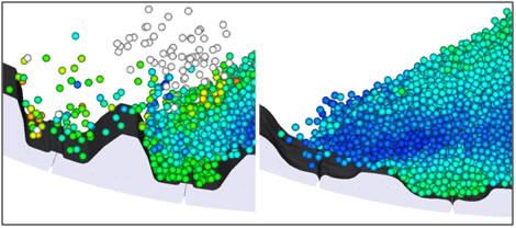
Tips:
To see a walk-through example of surface wear modification, refer to the following Workshops:
The replication settings, when coupled with Motion Frames and periodic motions, enable you to reproduce a geometry component at intervals along the path of the assigned motion. This can be useful for turning a single bucket into a full bucket elevator, for example (Figure 4).
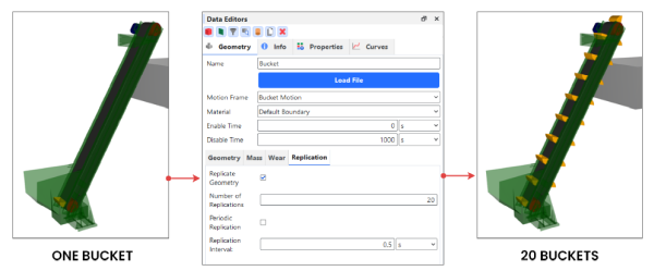
In this version of Rocky, replication can also be previewed in a Motion Preview window before processing the simulation. (See also Preview a Motion in 3D.)
Note: Geometry replication features are not compatible with free body motions. (See also About Creating and Applying Motion Frames.)
Tip: To see a walk-through example of replicating your geometries using periodic motions, refer to the following Workshop: Tutorial - Bucket Conveyor in the Rocky Tutorial Guide.
If you have enabled an external Module that affects your Geometries settings, you might also have a separate Modules sub-tab with additional settings that you can define (Figure 9). Refer to the Module's documentation (if provided) for more information. (See also Rocky Simulation Entities that can be Affected by Modules.)
Use the following figures and table to understand the various Geometry, Mass, Wear, and Replication parameters that you can set for an imported geometry.
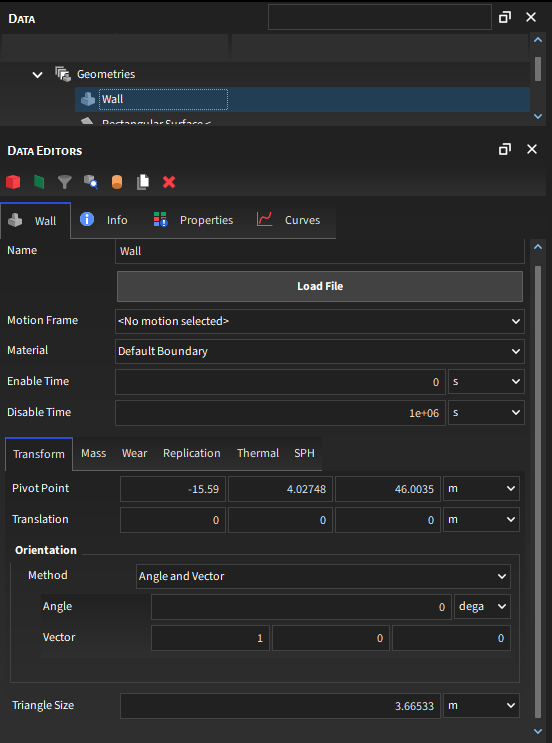
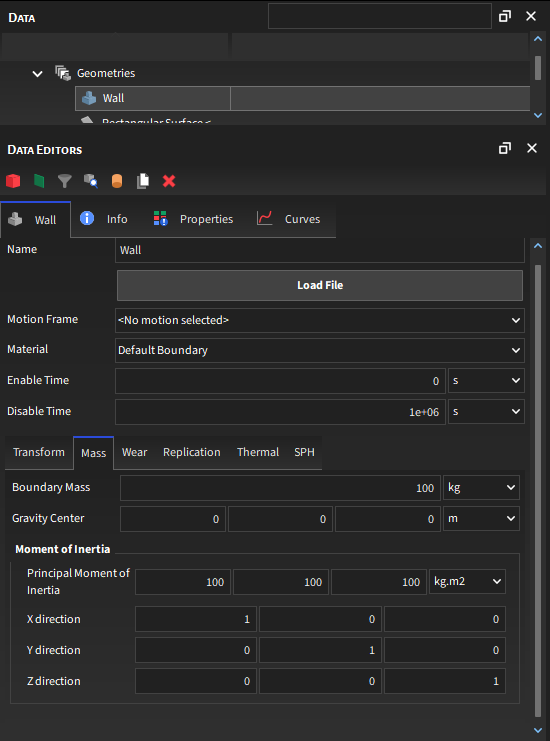
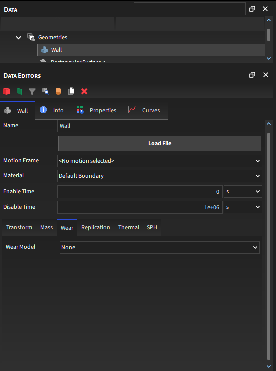
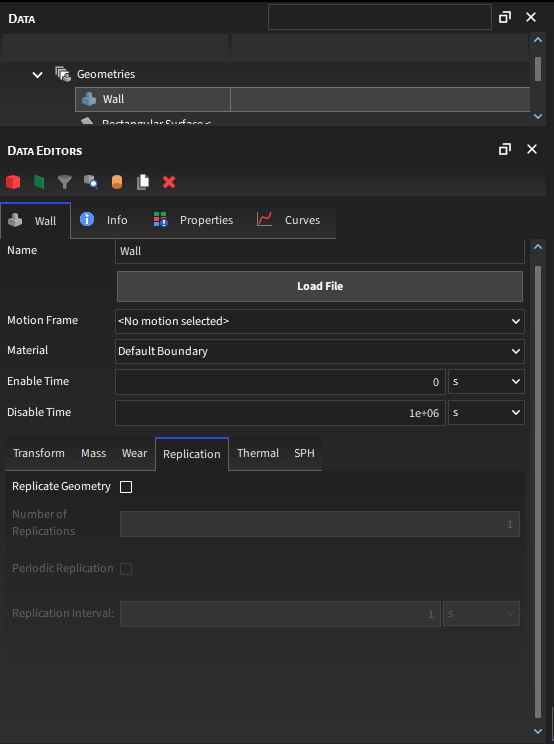
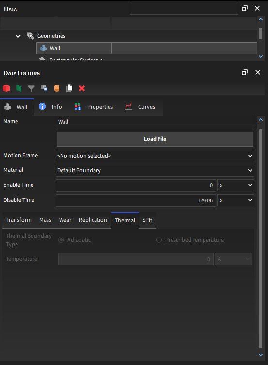
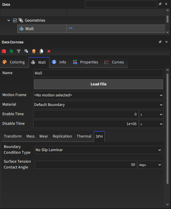

Table 3 : Imported wall parameter options (Geometry, Mass, Wear, and Replication subtabs)
Setting | Description | Range |
|---|---|---|
Name | Enables you to specify a unique identifier for the wall component. | No limit |
Motion Frame | Enables you to select which Motion Frame you want assigned to the geometry. (See also About Creating and Applying Motion Frames.) | Automatically provided |
Material | Defines the density and Young's Modulus of the wall component based upon the options you have set in the Materials list. (See About Modifying Material Compositions for more information.) When Thermal Model is enabled (see also About Physics Parameters), this also defines the specific heat and Poisson's ratio values, both of which are set in the Materials list. | List is based upon the Materials that have been defined |
Enable Time | The time you want the geometry to start interacting with particles during the simulation. Tip: To have the geometry interact with particles at simulation onset, keep Enable Time as zero (0). Note: If you choose to use parametric expressions in this field, know that only the resulting value and not the variables and/or mathematical functions you enter will be retained in any project copies you save for restart purposes. (See also I get a "Links removed" message when I save my project for restart purposes.) | Positive values Tip: Check the Status panel to ensure that any variables or mathematical functions you might use results in valid values. (See also Double-Click the Status Panel to Jump to the Appropriate UI Location.) |
Disable Time | The time you want the geometry to stop interacting with particles during the simulation. Tip: To have the geometry interact with particles for the duration of the simulation, keep Disable Time as 1e+06 or the maximum length of your simulation. Note: If you choose to use parametric expressions in this field, know that only the resulting value and not the variables and/or mathematical functions you enter will be retained in any project copies you save for restart purposes. (See also I get a "Links removed" message when I save my project for restart purposes.) | Positive values Tip: Check the Status panel to ensure that any variables or mathematical functions you might use results in valid values. (See also Double-Click the Status Panel to Jump to the Appropriate UI Location.) |
Transform | ||
Pivot Point | The coordinate location of the point around which the wall will pivot, as specified in the X, Y, and Z directions. Note: When Rocky calculates the transformation of coordinates of walls/surfaces, the operation of rotating the geometry around the pivot point comes first, then the translation operation is applied on those rotated coordinates. As a consequence, the pivot point that is inputted in the UI is the position of the pivot point before the translation, while the pivot point that appears in the 3D view is the pivot point after the translation operation. | No limit |
Translation | Enables you to move the geometry in the X, Y and Z directions. | Zero or Positive Values |
Orientation | Enables you to select how you want to define the orientation of the wall shape. Specifically:
| Angles; Angle and Vector; Basis Vectors. |
Orientation: Angle and Vector | ||
Angle | When Angle and Vector is selected for Orientation, this is the angle the wall will rotate around the defined Vector. | Any value |
Vector | When Angle and Vector is selected for Orientation, this is the X, Y, and Z components that define the vector around which the wall will rotate, using the defined Angle. | No limit but the values entered will be normalized |
Orientation: Basis Vector | ||
X direction | When Basis Vectors is selected for Orientation, this is the coordinate values defining the first of three directional vectors that together define the final orientation of the wall. Tip: To ensure correct results, make sure you define this vector as orthogonal (perpendicular) to the other two vectors. | No limit but, the values entered will be normalized |
Y direction | When Basis Vectors is selected for Orientation, this is the coordinate values defining the second of three directional vectors that together define the final orientation of the wall. Tip: To ensure correct results, make sure you define this vector as orthogonal (perpendicular) to the other two vectors. | No limit but,the values will be normalized |
Z direction | When Basis Vectors is selected for Orientation, this is the coordinate values defining the third of three directional vectors that together define the final orientation of the wall. Tip: To ensure correct results, make sure you define this vector as orthogonal (perpendicular) to the other two vectors. | No limit but,the values will be normalized |
Orientation: Angles | ||
Order | When Angles is selected for Orientation, this defines the order in which the three Rotation text fields will be applied. | XYZ; ZXY; YXZ; YZX; ZXY; ZYX. |
Local Angles | When Angles is selected for Orientation, this defines what coordinate system will be used as a basis for the angle specified. Specifically:
| Turns on or off |
Rotation | When Angles is selected for Orientation, this is the degree of wall rotation in each of the three directions specified by the Order provided. | Any value |
Triangle Size | Size of the triangular components into which the boundary is divided. This value is used both for refining the boundary mesh (this will not happen if the imported Triangle Size is already finer than this value) and for averaging purposes during wear and surface wear modification calculations. Therefore, in general, the smaller the Triangle Size, the more accurate the wear calculations but the longer the processing time. (See also View a Color Map of Wear on the Default Belt or Imported Geometry Itself and View Surface Wear Modification on an Imported Geometry.) | Positive values |
Mass | ||
Boundary Mass | When Free Body Translation or Free Body Rotation are defined for the Motion Frame applied to this geometry, this is the mass of the geometry. | Positive values |
Gravity Center | When Free Body Translation or Free Body Rotation are defined for the Motion Frame applied to this geometry, this is the location in coordinates of the center point of gravity for the geometry. This can only be visualized in a 3D view, and when t=0. | No limit |
Mass (Moments of Inertia) | ||
Principal Moment of Inertia | When Free Body Translation or Free Body Rotation are defined for the Motion Frame assigned to this geometry (see also About Creating and Applying Motion Frames), these are the principal moments of inertia along the X, Y, and Z axes defined below. | Positive values greater than but not equal to zero |
X direction | The X, Y, and Z components that define the X axis for the Principal Moment of Inertia. Note: This is based upon the global coordinate system. | No limit but the values entered will be normalized, and the base must be positive orthonormal |
Y direction | The X, Y, and Z components that define the Y axis for the Principal Moment of Inertia. Note: This is based upon the global coordinate system. | No limit but the values entered will be normalized, and the base must be positive orthonormal |
Z direction | The X, Y, and Z components that define the Z axis for the Principal Moment of Inertia. Note: This is based upon the global coordinate system. | No limit but the values entered will be normalized, and the base must be positive orthonormal |
Wear | ||
Wear Model | The calculation used to perform wear modifications of the geometry surface. Unless you have enabled a custom external Modules that defines a different Wear model, the only option listed will be Shear Work Proportionality (Archard's Law). This model works by ensuring that the volume of geometry removed is proportional to the shear wear applied to the geometry. | None; Shear Work Proportionality (Archard's Law) Note: If you have a Module that adds in an additional Wear law, you must use that law at least once in your simulation project if the Module is enabled. Refer to the Module's documentation (if provided) for more information. (See also Rocky Simulation Entities that can be Affected by Modules.) |
Volume/Shear Work Ratio | The amount of surface volume that is removed per shear work applied. Note: This is a calibration step that comes from real-world wear data you have collected using similar types of liners. | Positive values |
Replication | ||
Replicate Geometry | Enables Rocky to replicate the geometry along the path of the Motion Frame that is applied to it. This is useful for creating several exact copies of a geometry along the same movement path, such as turning a single pan into a full apron feeder, a single bucket into a full bucket conveyor (Figure 4), and so on. Works best in conjunction with periodic motions. (See also About Creating and Applying Motion Frames.) When used without periodic motions, the replicas will still start in different positions along the path of the Motion Frame, but will all eventually stop in the same final position (i.e., overlapping one another) when the motion frame's stop time is reached. | Turns on or off |
Number of Replications | Sets the amount of times (copies) you want the geometry to be replicated. | Positive integer values |
Periodic Replication | Determines how the time interval between geometry replications is set. Specifically, when:
These intervals may be useful for specifying gaps between buckets along a bucket conveyor, for example. | Turns on or off |
Replication Period | When Periodic Replication is enabled (checked), this sets the total amount of time during which geometry replications will occur. The interval between individual replications can be determined by dividing this value by the Number of Replications that is set. For example, if you set this value to 3 and Number of Replications is also 3, then the geometry will replicate every 1 s. | Positive values |
Replication Interval | When Periodic Replication is cleared (unchecked), this sets the amount of time between geometry replications. For example, if you set this value to 1, the geometry will be replicated every 1 s until the Number of Replications value has been achieved. | Positive values |
Modules | ||
(Varies) | These settings are specific to only certain external Modules and are therefore not documented in the Rocky User Manual. Refer to the Module's documentation (if provided) for more information. (See also Rocky Simulation Entities that can be Affected by Modules.) | (Varies) |
What would you like to do?
See Also:
Conveyors template are included in Rocky, allowing you to use Feed and Receiving conveyors without the need of importing a custom geometry. One of the benefits of using a default Conveyor is that you can easily adjust the speed of the conveyor itself, and even set it up to accelerate from or decelerate to a full stop, which is particularly useful for testing plant start-up or shut-down scenarios.
One of the main drawbacks of using a Conveyor template is that while you can certainly analyze the wear on the belt using color mapping (see also View a Color Map of Wear on the Default Belt or Imported Geometry Itself), default geometries, including Feed Conveyors and Receiving Conveyors, do not support showing surface wear modification (see also View Surface Wear Modification on an Imported Geometry) on the boundaries. So if you are interested in doing that kind of wear analysis, you will want to import a custom feed conveyor instead (see also Import Wall or Surface Geometries.).
Note: If you have enabled an external Module that affects your Conveyor template settings, you might also have a separate Modules sub-tab with additional settings that you can define (Figure 6). Refer to the Module's documentation (if provided) for more information. (See also Rocky Simulation Entities that can be Affected by Modules.)
To add a conveyor template to your simulation:
From the Data panel, right-click Geometries, and then do one of the following:
Point to Conveyor Templates, and then click either Create Feed Conveyor or Create Receiving Conveyor.
The item you chose is now listed alphabetically (case sensitive) in the Data panel below Geometries.
Repeat step 1 for as many default geometries that you want in your simulation.
Feed Conveyors come with a built-in inlet (equal to the size, location, and orientation of the top of the Feeder Box), and can be adjusted to account for different pulley and skirtboard sizes, belt and roll configurations, and more.
Note: You cannot set a fluid inlet in a Feed Conveyor template.
Use the figures and table below to understand the various parameters you can set for a default feed conveyor.
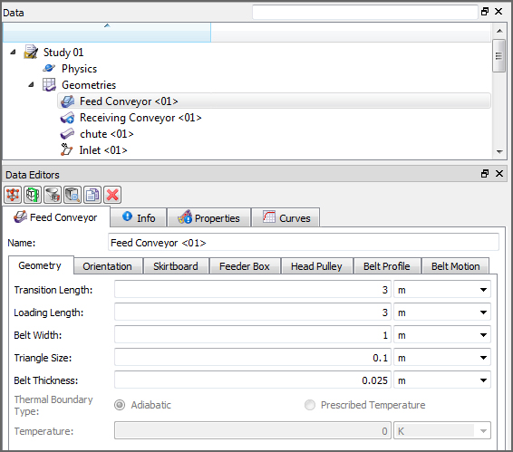
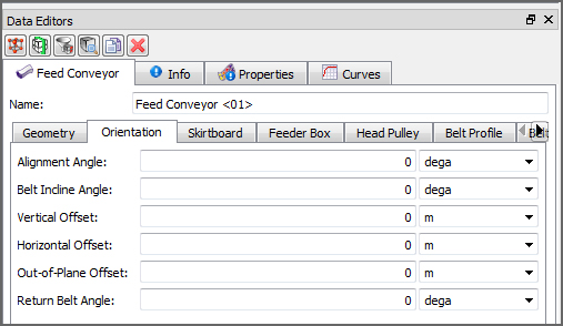
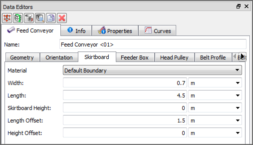
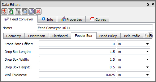
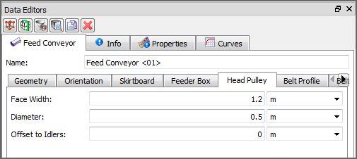
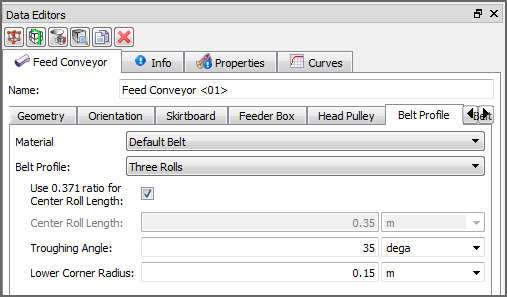
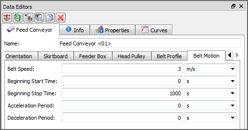
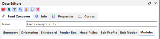
Table 1: Default Feed Conveyor parameter options (all tabs)
Setting | Description | Range |
|---|---|---|
Name | Enables you to specify a unique identifier for the geometry component. | No limit |
Geometry | ||
Transition Length | Length of the transition or ending portion of the conveyor belt. | Positive values |
Loading Length | Length of the loading or beginning portion of the conveyor belt. | Positive values |
Belt Width | Width of the conveyor belt. | Positive values |
Triangle Size | Size of the triangular components into which the boundary is divided. This value is used both for refining the boundary mesh (this will not happen if the default Triangle Size is already finer than this value) and for averaging purposes during wear calculations. Therefore, in general, the smaller the Triangle Size, the more accurate the wear calculations but the longer the processing time. (See also View a Color Map of Wear on the Default Belt or Imported Geometry Itself.) | Positive values |
Belt Thickness | Thickness of the conveyor belt. Affects visualization only; does not affect calculations. | Positive values |
Thermal Boundary Type | When Thermal Model is enabled (see also About Physics Parameters), this determines how heat conduction is calculated for the boundary. Specifically:
| Adiabatic; Prescribed Temperature |
Temperature | When Prescribed Temperature is selected, this sets the temperature value for the boundary. | Values above but not equal to 0 K (zero Kelvin) |
Orientation | ||
Alignment Angle | Angle the top (carry) part of the conveyor will be placed on the horizontal plane. | No limit |
Belt Incline Angle | Angle the conveyor will be placed on the vertical plane. | No limit |
Vertical Offset | Distance away from zero on the Y axis that the conveyor will be placed. | No limit |
Horizontal Offset | Distance away from zero on the X axis that the conveyor will be placed. | No limit |
Out-of-Plane Offset | Distance away from zero on the Z axis that the conveyor will be placed. | No limit |
Return Belt Angle | Angle the bottom (return) part of the conveyor will be placed on the horizontal plane. | No limit |
Skirtboard | ||
Material | Defines the density and Young's Modulus of the skirtboard based upon the options you have set in the Materials list. (See About Modifying Material Compositions for more information.) | List is based upon the Materials that have been defined |
Width | Width of the conveyor skirtboard. | Positive values |
Length | Length of the conveyor skirtboard. | Positive values |
Skirtboard Height | Height of the conveyor skirtboard. | Positive values |
Length Offset | Horizontal distance away from the beginning of the belt to place the skirtboard. | Positive values |
Height Offset | Vertical distance away from the belt to place the skirtboard. | Positive values |
Feeder Box | ||
Front Plate Offset | Length that the front plate will extend from the edge of the feeder box over the conveyor belt. | Positive values |
Drop Box Length | Length of the feeder box. | Positive values |
Drop Box Width | Width of the feeder box. | Positive values |
Drop Box Height | Height of the feeder box. | Positive values |
Wall Thickness | Thickness of the feeder box and skirtboard walls. | Positive values |
Head Pulley | ||
Face Width | Width of the conveyor pulley. | Positive values |
Diameter | Diameter of the conveyor pulley. | Positive values |
Offset to Idlers | Vertical distance away from the belt that the idlers will be placed. | No limit |
Belt Profile | ||
Material | Defines the density and Young's Modulus of the belt based upon the options you have set in the Materials list. (See About Modifying Material Compositions for more information.) | List is based upon the Materials that have been defined |
Belt Profile | Amount of rolls that support the conveyor belt. | 1, 2, 3, or 5 rolls |
Use 0.371 ratio for Center Roll Length | When 3 rolls are selected, automatically calculates center roll length as 0.371 of the Belt Width. | Turns on or off |
Center Roll Length | When 3 or 5 rolls are selected, this specifies the length of the center roll. | Positive values |
Troughing Angle | The degree by which the belt trough is formed between the side and center rolls. | Above but not equal to zero (0) degrees. Tip:The recommended range is 0 < 90 degrees. |
Lower Corner Radius | Radius of the inside corner between the center and side rolls. The bigger the value, the smoother the transition. | Positive values |
Side Roll Length | When 5 rolls are selected, this specifies the length of the two side rolls closest to the center roll. | Positive values |
Use 0.223 ratio for Roll Lengths | When 5 rolls are selected, automatically calculates the side roll length as 0.223 of the Belt Width. | Turns on or off |
Last Roll Angle | When 5 rolls are selected, this specifies the degree by which the belt trough is formed between the side and outer rolls. | 0 < 90 degrees |
Upper Corner Radius | When 5 rolls are selected, this specifies the radius of the inside corner between the side and outer rolls. The bigger the value, the smoother the transition. | Positive values |
Belt Motion | ||
Belt Speed | Full speed of the conveyor belt after it completes the Acceleration Period. | Positive values |
Beginning Start Time | The time you want the belt to begin moving. This is when the Acceleration Period begins. | Positive values |
Beginning Stop Time | The time you want the belt to begin stopping. This is when the Deceleration Period begins. | Positive values |
Acceleration Period | The length of time you want the belt to take to reach full Belt Speed. Acceleration starts at the Beginning Start Time and ends after the time period you specify here. | Positive values |
Deceleration Period | The length of time you want the belt to take to come to a full stop. Deceleration starts at the Beginning Stop Time and ends after the time period you specify here. | Positive values |
Modules | ||
(Varies) | These settings are specific to only certain external Modules and are therefore not documented in the Rocky User Manual. Refer to the Module's documentation (if provided) for more information. (See also Rocky Simulation Entities that can be Affected by Modules.) | (Varies) |
Receiving Conveyors can be adjusted to account for different belt and roll configurations, and more.
Use the following figures and table to understand the various parameters that you can set for a default receiving conveyor.
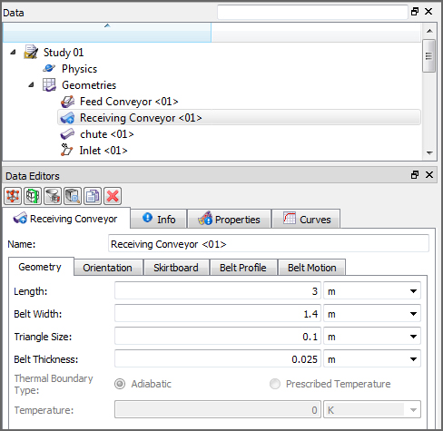
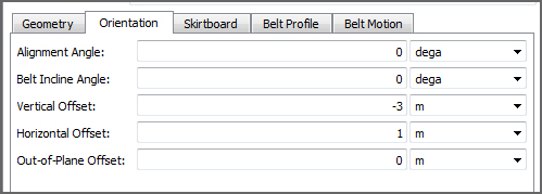
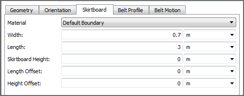
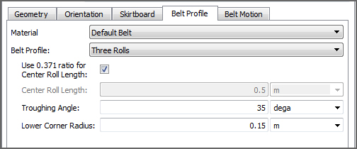
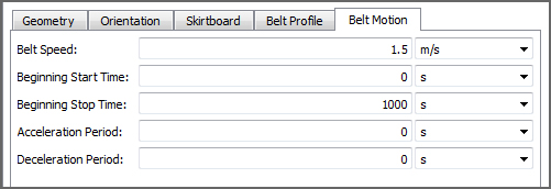

Table 2: Default Receiving Conveyor parameter options (all tabs)
Setting | Description | Range |
|---|---|---|
Name | Enables you to specify a unique identifier for the geometry component. | No limit |
Geometry | ||
Length | Length of the conveyor belt. | Positive values |
Belt Width | Width of the conveyor belt. | Positive values |
Triangle Size | Size of the triangular components into which the boundary is divided. This value is used both for refining the boundary mesh (this will not happen if the default Triangle Size is already finer than this value) and for averaging purposes during wear calculations. Therefore, in general, the smaller the Triangle Size, the more accurate the wear calculations but the longer the processing time. (See also View a Color Map of Wear on the Default Belt or Imported Geometry Itself.) | Positive values |
Belt Thickness | Thickness of the conveyor belt. Affects visualization only; does not affect calculations. | Positive values |
Thermal Boundary Type | When Thermal Model is enabled (see also About Physics Parameters), this determines how heat conduction is calculated for the boundary. Specifically:
| Adiabatic; Prescribed Temperature |
Temperature | When Prescribed Temperature is selected, this sets the temperature value for the boundary. | Values above but not equal to 0 K (zero Kelvin) |
Orientation | ||
Alignment Angle | Angle the top (carry) part of the conveyor will be placed on the horizontal plane. | No limit |
Belt Incline Angle | Angle the conveyor will be placed on the vertical plane. | No limit |
Vertical Offset | Distance away from zero on the Y axis that the conveyor will be placed. | No limit |
Horizontal Offset | Distance away from zero on the X axis that the conveyor will be placed. | No limit |
Out-of-Plane Offset | Distance away from zero on the Z axis that the conveyor will be placed. | No limit |
Skirtboard | ||
Material | Defines the density and Young's Modulus of the skirtboard based upon the options you've set in the Materials list. (See About Modifying Material Compositions for more information.) | List is based upon the Materials that have been defined |
Width | Width of the conveyor skirtboard. | Positive values |
Length | Length of the conveyor skirtboard. | Positive values |
Skirtboard Height | Height of the conveyor skirtboard. | Positive values |
Length Offset | Horizontal distance away from the beginning of the belt to place the skirtboard. | Positive values |
Height Offset | Vertical distance away from the belt to place the skirtboard. | Positive values |
Belt Profile | ||
Material | Defines the density and Young's Modulus of the belt based upon the options you've set in the Materials list. (See About Modifying Material Compositions for more information.) | List is based upon the Materials that have been defined |
Belt Profile | Amount of rolls that support the conveyor belt. | 1, 2, 3, or 5 rolls |
Use 0.371 ratio for Center Roll Length | When 3 rolls are selected, automatically calculates center roll length as 0.371 of the Belt Width. | Turns on or off |
Center Roll Length | When 3 or 5 rolls are selected, this specifies the length of the center roll. | Positive values |
Troughing Angle | The degree by which the belt trough is formed between the side and center rolls. | Above but not equal to zero (0) degrees. Tip:The recommended range is 0 < 90 degrees. |
Lower Corner Radius | Radius of the inside corner between the center and side rolls. The bigger the value, the smoother the transition. | Positive values |
Side Roll Length | When 5 rolls are selected, this specifies the length of the two side rolls closest to the center roll. | Positive values |
Use 0.223 ratio for Roll Lengths | When 5 rolls are selected, automatically calculates the side roll length as 0.223 of the Belt Width. | Turns on or off |
Last Roll Angle | When 5 rolls are selected, this specifies the degree by which the belt trough is formed between the side and outer rolls. | 0 < 90 degrees |
Upper Corner Radius | When 5 rolls are selected, this specifies the radius of the inside corner between the side and outer rolls. The bigger the value, the smoother the transition. | Positive values |
Belt Motion | ||
Belt Speed | Full speed of the conveyor belt after it completes the Acceleration Period. | Positive values |
Beginning Start Time | The time you want the belt to begin moving. This is when the Acceleration Period begins. | Positive values |
Beginning Stop Time | The time you want the belt to begin stopping. This is when the Deceleration Period begins. | Positive values |
Acceleration Period | The length of time you want the belt to take to reach full Belt Speed. Acceleration starts at the Beginning Start Time and ends after the time period you specify here. | Positive values |
Deceleration Period | The length of time you want the belt to take to come to a full stop. Deceleration starts at the Beginning Stop Time and ends after the time period you specify here. | Positive values |
Modules | ||
(Varies) | These settings are specific to only certain external Modules and are therefore not documented in the Rocky User Manual. Refer to the Module's documentation (if provided) for more information. (See also Rocky Simulation Entities that can be Affected by Modules.) | (Varies) |
What would you like to do?
See Also:
From the Data panel, under Geometries, select the name of the geometry that you want to edit. The parameters for that geometry are displayed in the Data Editors panel. The tab named with the type of geometry you selected (for example, Wall, "Surface", and so on) will be active.
From the Data Editors panel, enter the information you want on the active tab, being sure to select each of the various sub-tabs or dialogs that contain parameters you want to modify.
Tip: To set the same value for a parameter across multiple similar geometries, multi-select the geometries you want in the Data panel (SHIFT + left-click for a continuous group; CTRL + left-click for discontinuous items) and then change the values you want in the Data Editor panel. Only those parameters common across all selected geometries will be editable but any changes made will populate across the selected group.
See Also:
In cases where you need to analyze or otherwise make use of your rendered geometry component outside of Rocky, you may choose to export it to an .stl file. This applies to default Feed Conveyors, default Receiving Conveyors, and any geometry components that you have previously imported. Exporting a geometry at different times for further analysis is especially useful after your geometry surface has been modified by wear. (See also View Surface Wear Modification on an Imported Geometry.)
This export ability applies also to any User Processes created from a geometry component, which exports the shape of any (whole) geometry triangles that are selected by the User Process. (See also Export User Process Geometry Triangles to an STL File.)
Exporting a geometry component enables you to select which units you want to use when exporting (Figure 1).
If exporting worn geometries, ensure that you have selected what Timestep you want from the Time toolbar.
From the Data panel, under Geometries, right-click the component you want to export, point to Export, and then click Rendered Geometry.
From the Select output unit dialog, select from the Output Unit list the units you want, and then click OK.
From the Select target STL file dialog, click the drive or folder of the location to which you want to save the file.
In the File name box, enter a name for the file, and then click Save.
See Also:
If you import a surface into Rocky, you can also export it following the steps in To export a geometry component to an STL file:. However, it is not possible to export surfaces created inside Rocky.
From the Data panel, under Geometries, right-click the name of the geometry you want to remove, and then click Remove Geometry.
Tip: If you want to change out a geometry component for a different file, you can also choose to just replace the file. (See also Replace an Imported Geometry File.)
See Also:
From the Data panel, under Geometries, select the imported geometry component you want to replace.
From the Data Editors panel, select the Geometry tab and then click the Load File button.
From the Select file to import dialog, locate and select the geometry file you want to re-import, and then click Open.
From the File Import Info dialog, choose the import options you want, and then click OK
See Also:
Regions of Interest enable you to specify an area inside the simulation domain within which certain external Modules can perform custom calculations.
Tip: Unless you have enabled an external Module that makes use of a Region of Interest, you can skip this part of your Rocky setup.
What would you like to do?
See Also:
A Region of Interest (sometimes referred to as a "ROI") enables you to specify an area inside the simulation domain within which certain external Modules can perform custom calculations. The calculations within this "sub-domain" results in data that can be visualized and analyzed through other entities—such as Particles and Geometries—similar to how calculations in the main domain function.
Tip: Unless you have enabled an external Module that makes use of a Region of Interest, you can skip this part of your Rocky setup.
In this version of Rocky, there are two shape options you can define as a Region of Interest:
A Cube, which enables you to create a box-like shape.
A Cylinder, which enables you to create a full or partial cylindrical shape, with or without a center hole.
While both shapes have setups and appearances similar to those of their User Process cousins (see also Analyze Data within a Defined Shape), a Region of Interest shape is quite different in purpose and function as illustrated in Figure 1.
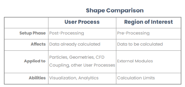
What would you like to do?
See Also:
The Cube Region of Interest enables you to define within the simulation boundaries a three dimensional box of whatever length, width, and height you want. In this way, you can limit the calculations of certain external Modules to only the domain selection contained within the box.
Tip: Unless you have enabled an external Module that makes use of a Region of Interest, you can skip this part of your Rocky setup.
Like Cube User Processes, you can use the colored directional handles (Figure 1) in a 3D View window to change the shape and location of the box (see also Use Colored Directional Handles), or you can define exact values in the Data Editors panel.
See the image and table below to learn more about the Cube Region of Interest.
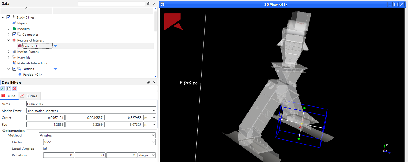
Table 1: Cube Region of Interest parameter options
Setting | Description | Range |
|---|---|---|
Name | Enables you to specify a unique identifier for the Region of Interest. Note: This same name will appear in the Data panel under Regions of Interest. | No limit |
Center | The X, Y, and Z coordinate locations of the cube's center point. | Any value |
Size | The length of the cube's three sides as specified in the X, Y, and Z directions. | Any value |
| Orientation | ||
Method | Enables you to select how you want to define the orientation of the cube shape. Specifically:
| Angles; Angle and Vector; Basis Vectors |
Method Angles | ||
Order | When Angles is selected for Orientation, this defines the order in which the three Rotation text fields will be applied. | XYZ; ZXY; YXZ; YZX; ZXY; ZYX |
Local Angles | When Angles is selected for Orientation, this defines what coordinate system will be used as a basis for the angle specified. Specifically:
| Turns on or off |
Rotation | When Angles is selected for Orientation, this is the degree of cube rotation in each of the three directions specified by the Order provided. | Any value |
Method Angle and Vector | ||
Angle | When Angle and Vector is selected for Orientation, this is the angle the cube will rotate around the Vector defined. | Any value |
Vector | When Angle and Vector is selected for Orientation, this is the X, Y, and Z components that define the vector around which the cube will rotate, using the Angle defined. | No limit but the values entered will be normalized |
Method Basis Vectors | ||
X direction | When Basis Vectors is selected for Orientation, this is the coordinate values defining the first of three directional vectors that together define the final orientation of the cube. Tip: To ensure correct results, make sure you define this vector as orthogonal (perpendicular) to the other two vectors. | No limit but the values entered will be normalized |
Y direction | When Basis Vectors is selected for Orientation, this is the coordinate values defining the second of three directional vectors that together define the final orientation of the cube. Tip: To ensure correct results, make sure you define this vector as orthogonal (perpendicular) to the other two vectors. | No limit but the values entered will be normalized |
Z direction | When Basis Vectors is selected for Orientation, this is the coordinate values defining the third of three directional vectors that together define the final orientation of the cube. Tip: To ensure correct results, make sure you define this vector as orthogonal (perpendicular) to the other two vectors. | No limit but the values entered will be normalized |
What would you like to do?
See Also:
The Cylinder Region of Interest enables you to define within the simulation boundaries a three dimensional analysis tube, arch, or slice of whatever radius and height you want, and with or without a center hole. (See Figure 3 below for examples.) In this way, you can limit the data an external Modules calculates to only the selection contained by the shape you determine. The method is particularly useful for analyzing certain areas of equipment with round components, such as mills and pipes.
Note: Unlike Cylinder User Processes, which can be elliptical in shape (see also About the Cylinder User Process), Region of Interest Cylinders must only be perfectly round.
See the images and table below to learn more about the Cylinder Region of Interest.
What you set for your Initial and Final Arc Angle values determine how far around the Y axis the arc for the cylinder will be drawn. Cylinder Arc Angles follow the right-hand rule: when the Y axis points outside the screen (from the Fit menu, select Camera Preset: +Y), no matter whether you enter a positive or negative value for the Final parameter, the arc will be drawn from the Initial value counterclockwise to your Final value. (See Figure 1 below for an illustration.)
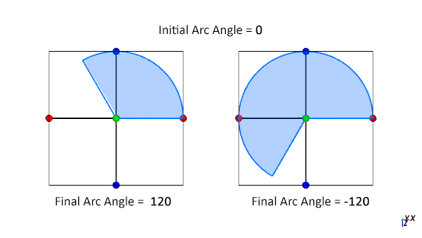
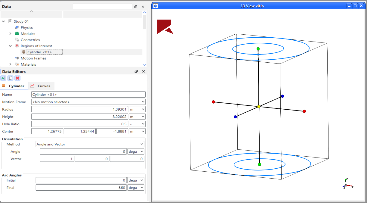
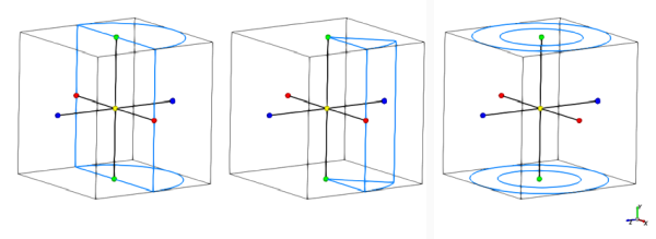
Table 1: Cylinder Region of Interest parameter options
Setting | Description | Range |
|---|---|---|
Name | Enables you to specify a unique identifier for the Region of Interest. Note: This same name will appear in the Data panel under Regions of Interest. | No limit |
Center | The X, Y, and Z coordinate locations of the shape's center point. | Any value |
Radius | The size of the cylinder's outer radius. | Any value |
Height | The size of the shape's dimension in the Y direction. | Any value |
Hole Ratio | The percentage of volume that the center hole through the cylinder will take up. | 0-1 |
| Orientation | ||
Method | Enables you to select how you want to define the orientation of the cylinder shape. Specifically:
| Angles; Angle and Vector; Basis Vectors |
Method Angles | ||
Order | When Angles is selected for Orientation, this defines the order in which the three Rotation text fields will be applied. | XYZ; ZXY; YXZ; YZX; ZXY; ZYX |
Local Angles | When Angles is selected for Orientation, this defines what coordinate system will be used as a basis for the angle specified. Specifically:
| Turns on or off |
Rotation | When Angles is selected for Orientation, this is the degree of cylinder rotation in each of the three directions specified by the Order provided. | Any value |
Method Angle and Vector | ||
Angle | When Angle and Vector is selected for Orientation, this is the angle the cylinder will rotate around the Vector defined. | Any value |
Vector | When Angle and Vector is selected for Orientation, this is the X, Y, and Z components that define the vector around which the cylinder will rotate, using the Angle defined. | No limit but the values entered will be normalized |
Method Basis Vectors | ||
X direction | When Basis Vectors is selected for Orientation, this is the coordinate values defining the first of three directional vectors that together define the final orientation of the cylinder. Tip: To ensure correct results, make sure you define this vector as orthogonal (perpendicular) to the other two vectors. | No limit but the values entered will be normalized |
Y direction | When Basis Vectors is selected for Orientation, this is the coordinate values defining the second of three directional vectors that together define the final orientation of the cylinder. Tip: To ensure correct results, make sure you define this vector as orthogonal (perpendicular) to the other two vectors. | No limit but the values entered will be normalized |
Z direction | When Basis Vectors is selected for Orientation, this is the coordinate values defining the third of three directional vectors that together define the final orientation of the cylinder. Tip: To ensure correct results, make sure you define this vector as orthogonal (perpendicular) to the other two vectors. | No limit but the values entered will be normalized |
| Arc Angles | ||
Initial Arc | The initial degree point around the Y axis that the circular portion of the cylinder will be drawn. When the Y axis points outside the screen, the resulting arc will be drawn from the initial angle counterclockwise to the final angle. Tip: To draw a full cylinder, keep this value zero (0) and set Final to 360. | Any value |
Final Arc | The final degree point around the Y axis that the circular portion of the cylinder will be drawn. when the Y axis points outside the screen, the resulting arc will be drawn from the initial angle counterclockwise to the final angle. Tip: To draw a full cylinder, set this value to 360 and keep Initial at zero (0). | Any value |
What would you like to do?
See Also:
Ensure you have enabled an external Module that makes use of Regions of Interest.
Tip: If you do not plan to enable an external Module that makes use of Regions of Interests, then you do not need to add a Region of Interest to your simulation.
From the Data panel, right-click Study, select Regions of Interest and then create the shape you want to.
Note: The Regions of Interest entity shows up when you create a ROI, otherwise it will be hidden from the Study.
From the Data panel, select the newly created ROI below Regions of Interest, and from the Data Editors panel, on the shape tab for the item (Cube or Cylinder), enter the options you want.
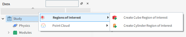
Tip: In the 3D View window (see also Create and Modify a 3D View), you can also move and resize the Region of Interest area by clicking and dragging the handles (colored dots). (See also Use Colored Directional Handles.)
See Also:
From the Data panel, under Regions of Interest, select the entry that you want to change.
From the Data Editors panel, do one of the following:
To edit the entity, from the shape tab for the item (Cube or Cylinder), change the settings you want.
To remove the entity, click the Remove button.
See Also:
Motion Frames are the method by which you enable geometry components (wall or surfaces)-or when coupled with Particle Custom Inlets to translate, rotate, vibrate, swing, and/or move during your simulation. If a surface is attached to an Inlet/Outlet, this component will also inherit the motion assigned to the geometry. You first define your desired movement within the Motion Frame, and then assign the Motion Frame to the geometry or Particle Custom Inlet you want to move. After setting up and applying your Motion Frames, it is a good idea to preview your motions in a Motion Preview window before processing the simulation.
Because the crushing movement can be more complicated to set up than other kinds of movements, Rocky also enables you to create a Cone Crusher Frame, which works similarly to a Motion Frame but has its own unique parameters.
What would you like to do?
Learn more About Creating and Applying Motion Frames
Learn more about Using Motion Frames to Create Specific Movements
See Also:
Creating and applying one or more Motion Frames to an imported geometry-or when coupled with Custom Inputs, the "frozen" portion of a frozen Fiber-enables that component to move or animate during your simulation. You can create simple movements-including translation, rotation, vibration, and swinging motions-or more complex movements by nesting several Motion Frames, and/or by enabling six degrees of freedom (6DOF) functionality (also known as Free Body Motion). Crushing movements are defined with a separate kind of frame, called a Cone Crusher Frame, but are created, applied, and previewed in the same manner as a standard Motion Frame. (See also About Creating and Applying Cone Crusher Frames to Imported Geometries.)
Motion Frames can be set only for imported geometries and Custom Inputs when set with frozen Fiber particle set, but it is important to note that all default conveyors included within Rocky have Keep in place (Global) translation values already enabled. This is how the particles appear to move along the conveyor belt even though the conveyor surface itself appears static.
Motion Frames work best in conjunction with the Motion Preview window as it allows you to view and test your motions before processing your simulation. (See also Preview a Motion in 3D.)
Note: When a geometry is disabled in Rocky by increasing its enable time (See also Imported Wall Parameters.), it is removed from the particle contact search process. However, if the geometry is associated with a motion frame, its position and orientation are still updated in accordance with the motion frame's dynamics. The geometry's mass properties are accounted for in the calculation of motion frame reactions, ensuring consistency in the simulation's overall dynamics.
Periodic Translation (Vibration) and Periodic Rotation (Pendulum) motions are defined by specifying the amplitude and frequency values along a sine wave. The amplitude defines how far from the center point the movement translates (or rotates) and the frequency defines how many complete wave cycles will occur per second. The point along the sine wave period at which the motion begins along the sine wave is defined by the Initial Phase value. An Initial Phase value of zero degrees (default) causes the sine wave to start at the center point of the motion (Figure 1). For a simple linear vibration moving back and forth along the X axis, the frame would start at the zero position, move to the right most limit (maximum amplitude), reverse direction past the zero position to the left most limit (minimum amplitude), and then complete the cycle by reversing direction again to the zero (or 360 degree) position.
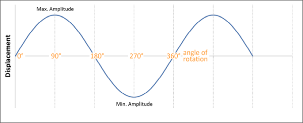
By comparison, changing the Initial Phase value to 90 degrees moves the starting point of the sine wave to the maximum amplitude, or in the simple linear vibration example, the right-most limit along the X axis (Figure 2). In this example, the frame would start its motion at the right-most limit along the X axis, then reverse direction past the zero position to the left most limit (minimum amplitude), and then reverse again to end its cycle at the right-most limit position.
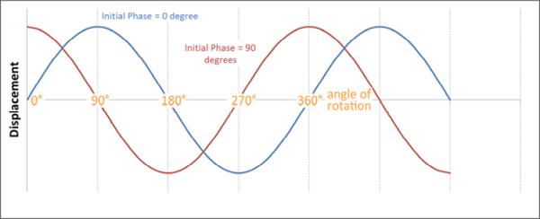
Changing the Initial Phase can be useful in cases where you want the center of the motion to remain the same but want the motion itself to begin from a non-center position. This is especially useful when combining two motions to create a complex motion.
For example, to create a circular vibration motion along the XY axes, you would create two separate vibration motions: the first along the X axis with Initial Phase at zero degrees, and the second along the Y axis with the Initial Phase at 90 degrees. This enables the vibration along the Y axis to start at its maximum (highest) position at the same time the vibration along the X axis begins its movement to the right from its center point. The combination of these two motions creates the desired circular vibration motion.
Tip: To see a walk-through example that uses vibration motions, refer to the following Workshop:
Tutorial - Vibrating Screen in the Rocky Tutorial Guide.
See Also:The [Webinar] Analyzing Vibrating Screen Equipment Efficiency Using Particle Simulation and the [Presentation] Practical Aspects of Vibrating Screen Simulation with DEM Test.
Periodic motions enables you to loop or repeat a set of motions within your simulation. When Enable Periodic Motion is turned on for a frame, the full list of motions contained within that frame will be repeated as soon as the motion with the last Stop Time completes. The amount of time between the earliest motion's Start Time and the latest motion's Stop Time is saved within Rocky as the periodic motion period.
This periodic motion period is useful to know when setting geometry replication as it can help you define your Replication Interval. To include an evenly spaced copy of the geometry along your periodic motion path, the Replication Interval should be equal to the periodic motion period divided by the Number of Replications you have defined.
Tip: To see a walk-through example that includes both periodic motions and geometry replication, refer to the following Workshop: Tutorial - Bucket Conveyor in the Rocky Tutorial Guide.
Free body motions, including Free Body Translation and Free Body Rotations, enable the frame to move freely in response to outside forces. These forces can come from particle contacts, gravity, or from an additional force that you prescribe through the Additional Force or Additional Moment motions, the Spring-Dashpot Force or Spring-Dashpot Moment motions, or the Linear Time Variable Force or Linear Time Variable Moment motions.
Free body motions do not currently respond to other boundary interactions, nor are they directly affected by CFD fluid flow. So setting an object to drop freely onto another object from some height will cause the object to fall through the other object. Having that same object drop freely onto a bed of particles, however, will cause the object to displace the particles and slow the object's falling as expected.
So too with CFD coupling simulations. Setting (on the Rocky side only) a flap-like object affixed at its top to rotate freely against a flow of fluid from the CFD side will cause the fluid to run straight through the flap without any movement. Having that same fluid carry a flow of particles, however, will cause the flowing particles to move the flap due to CFD fluid forces acting upon the particles, and not from the fluid forces over the geometry. Note: Geometries that are represented on both the DEM and CFD sides of a coupling simulation should not use free body motions. Rather, these geometries should use only the Fluent Motion Frame that is automatically created when the Fluent case is imported into Rocky. (See also About Importing Movements from Fluent section below.)
An Additional Force, Spring-Dashpot Force, or Linear Time Variable Force can be added to a Free Body Translation motion in cases where you want an additional force in a given direction to affect the translation, and you want that force to be considered in the motion calculation along with the weight, gravity, particle interactions.
For example, to simulate a car tire rolling along a bed of particles, aside from setting Free Body Translation and Free Body Rotation motions to simulate the horizontal translation and rotation of the tire, you could also add an Additional Force to account for the forward motion of the car itself. In this way, the acceleration and velocity of the translation will be affected by the particles and gravity values: given the same force applied, the car moves slower in sticky mud and faster when on dry road. If only a Translation were given instead of a combined Additional Force and Free Body Translation, the velocity of the translation would remain constant no matter the conditions of the other particles and forces coming into contact with it.
So too, an Additional Moment, Spring-Dashpot Moment, or Linear Time Variable Moment can be added to a Free Body Rotation motion in cases where you want an additional moment (or torque) in a given direction to affect only the rotation, and you want that additional torque to be included along with gravity and particle interactions in the motion calculation.
Free body motions can also have range limits applied to restrict free movement in a given direction.
Important: In order to preview a free body motion in the Motion Preview window or start processing the simulation, ensure there is a geometry component in the project that has the free body motion associated to it; otherwise, you will get an error.
In this release of Rocky, you are able to add many more types of concurrent free body motions and Frames, including nested Frames, as long as free body motions of the same type (Translation or Rotation) and direction do not overlap in time. Tip:See Geometry Limitations for an updated list of what to be aware of when working with Motion Frames that use Free Body motions.
In this version of Rocky, the Motion Preview window will preview the effects of gravity and any additional (prescribed) forces/moments that you define for free body motions, but will not be able to predict motions as a result of interactions with particles.
Note: Free body motions are not compatible with geometry replication features.
Tip: To see walk-through examples that use free body motions, refer to the following Workshops:
Important: Once the geometry has a free body motion you must correctly define the Boundary Mass, Gravity Center an Moment of Inertia properties to avoid issues.
Free Body Translation: Tutorial - Drop Weight Test in the Rocky Tutorial Guide
Free Body Rotation and Spring Dashpot Moment: Workshop 06 - High Pressure Grinding Rolls (HPGR)
2-Way coupling simulations between Ansys Fluent and Rocky (See also About Using the 2-Way Fluent Method) will now support Fluent's Moving Meshes for simple translation and/or simple rotation movements. For geometry movements that are represented on both the DEM and CFD sides, this ability helps ensure that the translation or rotation motions are kept the same in both programs. Multiple zones can be imported.
To enable this ability, the desired translation and/or rotation motion should be represented only on the Fluent side using Moving Meshes. Once these settings are saved into the Fluent CAS (CAS.H5 or CAS.GZ) file, that file is then imported into the Rocky project as part of the Fluent Two Way Coupling process, which then automatically turns the Fluent Moving Meshes information into new Rocky Motion Frame entries, one per Cell Zone with motions you have defined.
Important: If you decide to use expressions when defining your moving meshes in Fluent, Rocky will support this but will be unable to automatically replicate the Fluent motions for you in Rocky. In these particular cases, you must ensure that you manually create Motion Frames in Rocky that replicate the geometry movement in Fluent as closely as possible.
After the Motion Frames are created (either automatically by Rocky or manually by you), they need to be assigned to the appropriate geometry components within Rocky. These can be identical to the Fluent geometries if they were imported into Rocky from the Fluent CAS, CAS.H5, or CAS.GZ file, or can be completely different geometries that need to maintain the same motions as in Fluent, depending upon your simulation goals.
Unlike other Motion Frames created in Rocky, the parameters of any Fluent Motion Frames that were automatically created by Rocky will be disabled but still visible in the UI. This is to ensure the movements between the two programs are kept the same.
In order to create complex motions, Rocky allows you to nest motion frames under other motion frames. By doing so, the nested frame (child) becomes linked to the frame above it in the tree (parent). The child motion frame will move together with the parent motion frame and will also prescribe its own motions.
Because of this, only the child frame in a nested frame situation will be assigned to a geometry, as the child inherits its parent's motions in combination with its own motions.
Figure 3 below shows an example of a two child frames (Frame <01> <01> and Frame <01> <02>) nested beneath a parent frame (Frame <01>).
Tip: To see a walk-through example of nested motion frames, refer to the following Workshop:
Like any other Data panel item, you can duplicate an individual Motion Frame to create an exact copy of it (see also Duplicate a Data Panel Item). This exact copy includes any nested or child Frames that exist underneath the Frame that you are copying.
In Figure 3 below, Frame <01> <01> and Frame <01> <02> are nested or child Frames of Frame <01>. When Frame <01> is duplicated, both child Frames are duplicated as well (Figure 4), so that the new Frame <02> includes two child Frames: Frame <02> <01> and Frame <02> <02>.
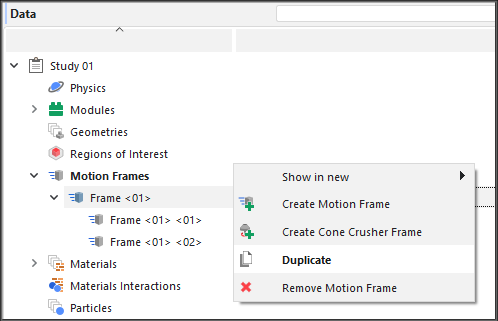
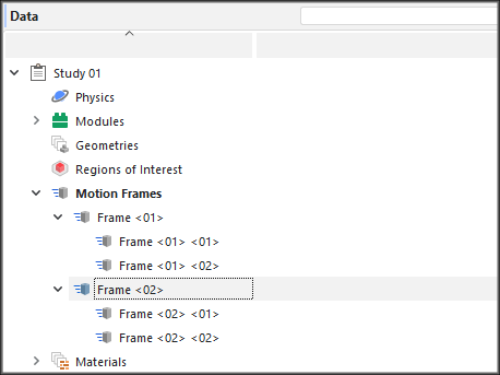
Motion Frames that are active at the time a processed simulation is saved for restart purposes (see also Save a Copy of a Partially Processed Simulation for Restart Purposes) will be copied to the new simulation, and will retain their original geometry assignments. However, even though the geometries using the frames can be removed from the copy, the copied frames themselves cannot be removed from the copy. These copied frames will also only allow changes to the Stop Time field for the existing motion (as long as the copied motion hasn't completed yet, meaning the Stop Time value is positive); new motions can be added to the existing frame, however, by clicking the Add Motion button.
In addition, only new motion frames can be assigned to new geometries in the copy; newly added geometries cannot be assigned frames copied from the original simulation, and geometries with motion frames copied from the original simulation cannot be assigned newly added motion frames. (See also About Changing Geometries and/or Particles in a Partially Processed Simulation.)
Be aware that if you choose to use parametric expressions in either the Start Time or Stop Time fields of your original simulation project, know that only the resulting values and not the variables and/or mathematical functions you entered will be retained in the project copy you save for restart purposes. (See also I get a "Links removed" message when I save my project for restart purposes.)
Each Motion Frame has its own orientation reference (i.e., coordinate system) upon which its movements are based. The current (i.e., instantaneous) orientation is represented in the Motion Preview window by the axis for the Frame.
In this version of Rocky, all Frames use only an implicit "local" reference, which uses the current orientation of the selected Frame to define the next movement. In this way, the reference is always moving along with the Frame.
Tip: In this version of Rocky, it is no longer possible to set a "parent" reference for a frame. However, you can recreate similar "parent" reference behavior by using nested Frames.
Note: When opening a project created in an older version of Rocky, any Frames with references set to "parent" must be modified so that they behave correctly in the "local" reference. See also I get "reference" errors in my Motion Frames when I open an older project.
You are able to assign a Motion Frame to Inlets or Outlets for particles or fluid. To do that you need to add a Motion Frame to the surface that is attached to that Inlet or Outlet (see also About Adding and Editing Inlets and Outlets).
You can also add Motion Frames to a Particle Custom Inlet when Rocky detects that the Particle set assigned to the Particle Custom Inlet is a multi-element frozen Fiber one. In these cases, the frozen Segments of the injected fibers will move according to the definition of the motion frame assigned.
See also Apply a Motion Frame to a Geometry. See also Apply a Motion Frame to a Custom Input.
User processes created for post-processing, such as cubes and cylinders, can now use motion frames to move around the domain and extract data while following geometries or particles. (see also Filter Views and Data with User Processes).
See also Apply a Motion Frame to a User Process.
See the images and tables below to understand how to create and apply Motion Frames to your imported geometries and Particle Custom Inlets.
Table 1: Motion Frames parameters (Main Entity)
|
Setting |
Description |
Range |
|---|---|---|
|
Default axes size |
Sets the size of the axes used to represent the Motion Frames in the Motion Preview window. Changing the size is useful in cases where the geometries are significantly bigger or smaller than the motion axes, as seeing the axes in relation to the movement of the geometry is critical to understanding and verifying the movement setup. Affects all Motion Frames axes in the project. (See also Preview a Motion in 3D.) Note: The axes for Motion Frames are different than the axes for the windows themselves; the latter have their own display settings that you can modify. (See also About Using the Window Editors Panel to Change the Window Axes Displays.) |
Positive value |
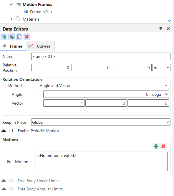
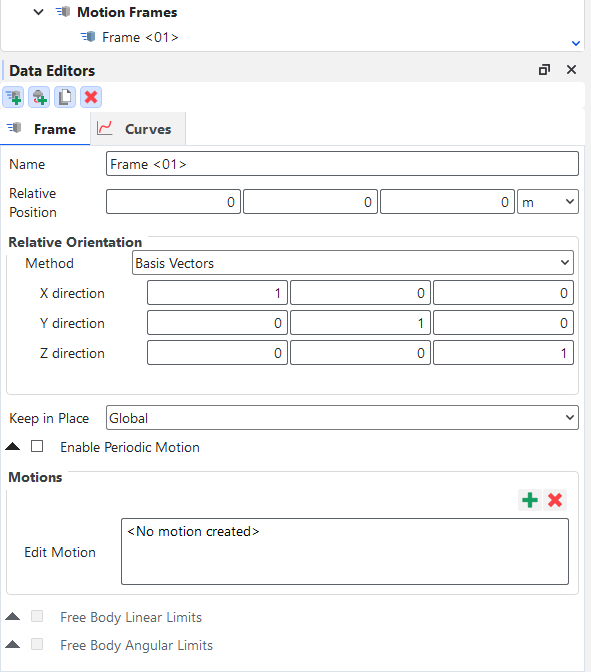
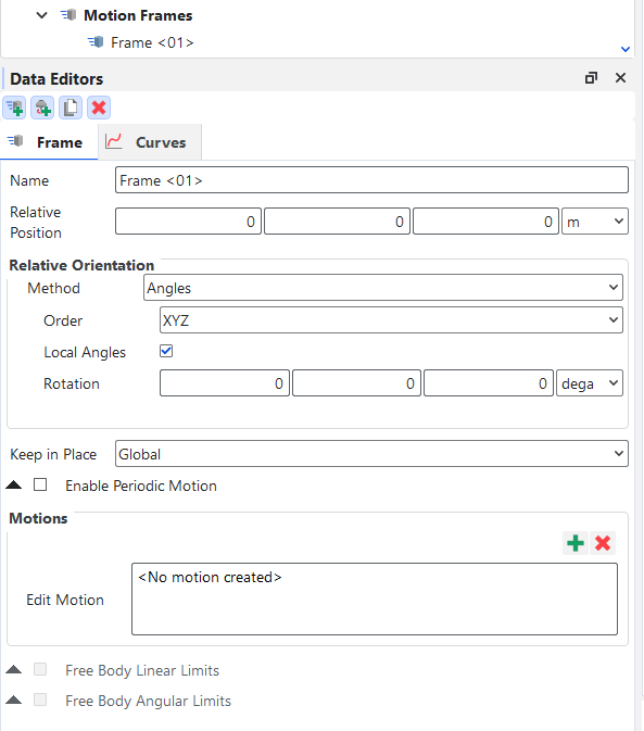
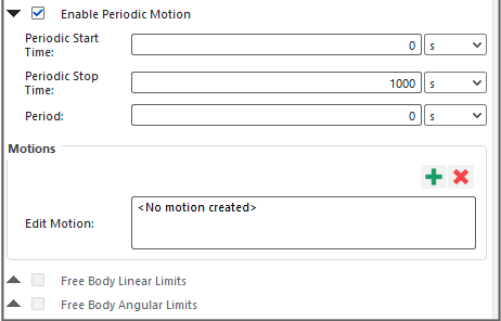
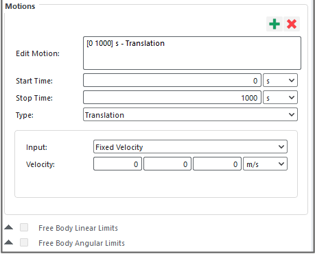
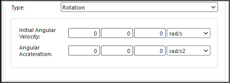
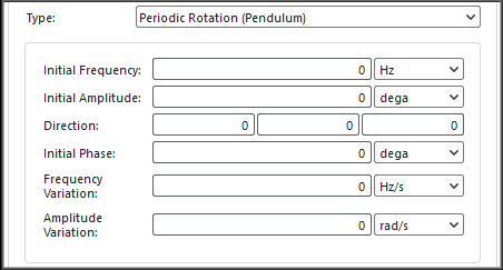
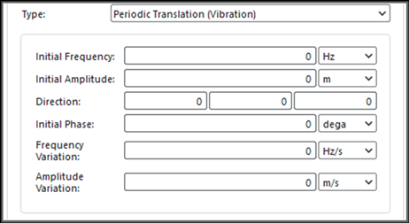
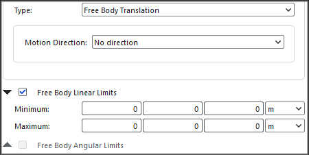
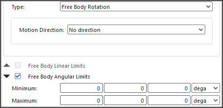
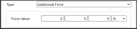
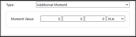
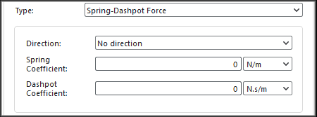
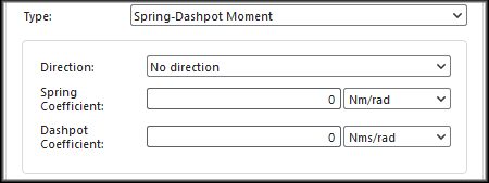
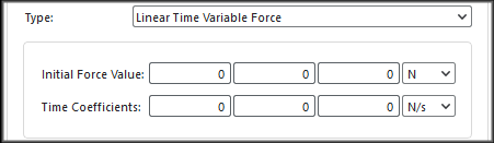
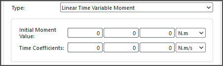
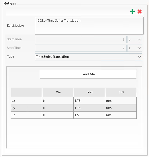
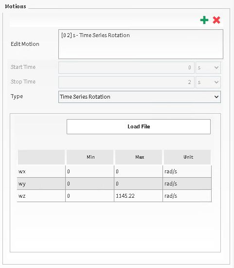
Table 2: Motion Frames parameters (Individual Frames)
Setting | Description | Range |
|---|---|---|
Name | Enables you to set a unique identifier for the selected motion frame. Note: When importing movements from Fluent, this will be equal to the Zone Name that was set for the Cell Zone in Fluent. | 99 character limit |
Relative Orientation | Enables you to select how you want to define the orientation of the motion frame shape. Specifically:
| Angles; Angle and Vector; Basis Vectors. Angle and Vector; Basis Vectors. |
Relative Orientation Angle and Vector | ||
Angle | When Angle and Vector is selected for Orientation, this is the angle the motion frame will rotate around the Vector defined. | Any value |
Vector | When Angle and Vector is selected for Orientation, this is the X, Y, and Z components that define the vector around which the motion frame will rotate, using the Angle defined. | No limit but the values entered will be normalized |
Relative Orientation Basis Vector | ||
X direction | When Basis Vectors is selected for Orientation, this is the coordinate values defining the first of three directional vectors that together define the final orientation of the motion frame. Note: To ensure correct results, make sure you define this vector as orthogonal (perpendicular) to the other two vectors. | No limit but,the values entered will be normalized |
Y direction | When Basis Vectors is selected for Orientation, this is the coordinate values defining the second of three directional vectors that together define the final orientation of the motion frame. Note: To ensure correct results, make sure you define this vector as orthogonal (perpendicular) to the other two vectors. | No limit but,the values entered will be normalized |
Z direction | When Basis Vectors is selected for Orientation, this is the coordinate values defining the third of three directional vectors that together define the final orientation of the motion frame. Note: To ensure correct results, make sure you define this vector as orthogonal (perpendicular) to the other two vectors. | No limit but,the values entered will be normalized |
Relative Orientation Angles | ||
Order | When Angles is selected for Orientation, this defines the order in which the three Rotation text fields will be applied. | XYZ; ZXY; YXZ; YZX; ZXY; ZYX. |
Local Angles | When Angles is selected for Orientation, this defines what coordinate system will be used as a basis for the angle specified. Specifically:
| Turns on or off |
Rotation | When Angles is selected for Orientation, this is the degree of cube rotation in each of the three directions specified by the Order provided. | Any value |
Keep in Place | Specifies whether or not the motion frame to which the frame is assigned will appear to move physically from one location to another. Specifically:
Notes:
See also I get "Displacement" errors in my Motion Frames when I open an older project. | Turns on or off |
Enable Periodic Motion | Enables the motion(s) defined for the selected frame to be repeated or looped for a defined period within the simulation. (See also Use Motion Frames to Enable Geometry Motions to be Repeated.) | Turns on or off |
Periodic Start Time | When Enable Periodic Motion is selected, this defines the amount of delay after the motion(s) Start Time and Stop Time to begin and end the motion to be repeated. Specifically:
| Positive values |
Periodic Stop Time | When Enable Periodic Motion is selected, this defines the time during the simulation when the motion(s) will stop, regardless of what is set for Stop Time. Specifically:
Tip: To ensure that the periodic motion continues for the entire simulation, keep this value set to the default (1000 s) or set it higher than your simulation duration. | Positive values |
Period | When Enable Periodic Motion is selected, this defines how much of the original motion(s) will be repeated. Specifically:
| Positive values |
Edit Motion | Lists the individual motions you have defined for the selected motion frame. Motions are automatically named in accordance with the following method: [StartTime StopTime]s - Type | Automatically determined |
Start Time | The time you want the selected motion to begin. Note:If you choose to use parametric expressions in this field, know that only the resulting value and not the variables and/or mathematical functions you enter will be retained in any project copies you save for restart purposes. (See also I get a "Links removed" message when I save my project for restart purposes.) | Positive values Tip: Tip: Check the Status panel to ensure that any variables or mathematical functions you might use results in valid values. (See also Double-Click the Status Panel to Jump to the Appropriate UI Location.) |
Stop Time | The time you want the selected motion to end. Note: Any gaps of time between multiple motions will be interpreted as no movement. Note: If you choose to use parametric expressions in this field, know that only the resulting value and not the variables and/or mathematical functions you enter will be retained in any project copies you save for restart purposes. (See also I get a "Links removed" message when I save my project for restart purposes.) | Positive values Tip: Check the Status panel to ensure that any variables or mathematical functions you might use results in valid values. (See also Double-Click the Status Panel to Jump to the Appropriate UI Location.) |
Type | Defines the type of movement. Specifically:
| Translation; Rotation; Periodic Rotation (Pendulum); Periodic Translation (Vibration); Free Body Translation; Free Body Rotation; Additional Force; Additional Moment; Spring-Dashpot Force; Spring-Dashpot Moment; Linear Time Variable Force; Linear Time Variable Moment |
Translation Parameters | ||
Input | Determines what velocity and acceleration values you want the motion to consider. Specifically:
| Fixed Velocity; Initial and Final Velocity; Initial Velocity and Acceleration |
Velocity | When Fixed Velocity is chosen for Input , this enables you to set a single translational velocity in the X, Y, and Z directions respectively. | Any value |
Initial Velocity | When Initial and Final Velocity or Initial Velocity and Acceleration is chosen for Input, this sets the starting translational velocity of the selected motion as defined in the X, Y, and Z directions respectively. A positive or negative value will prescribe the orientation of the movement over a given direction. | Any value |
Final Velocity | When Initial and Final Velocity is chosen for Input, this sets the ending translational velocity of the selected motion as defined in the X, Y, and Z directions respectively. A positive or negative value will prescribe the orientation of the movement over a given direction. | Any value |
Acceleration (computed) | When Initial and Final Velocity is chosen for Input, this displays the amount of acceleration in the X, Y, and Z directions respectively that Rocky calculates is required to achieve the Final Velocity given the Initial Velocity value. | Display only; values are calculated by Rocky |
Acceleration | When Initial Velocity and Acceleration is chosen for Input, this sets the amount of acceleration of the selected motion as defined in the X, Y, and Z directions respectively. | Any value |
Final Velocity (computed) | When Initial Velocity and Acceleration is chosen for Input, this displays the final velocity in the X, Y, Z directions respectively that Rocky calculates given both the Initial Velocity and Acceleration values. | Display only; values are calculated by Rocky |
Rotation Parameters | ||
Initial Angular Velocity | Sets the starting rotational (angular) velocity of the selected motion as defined in the X, Y, and Z directions respectively.
| Any value |
Angular Acceleration | Sets the amount of rotational (angular) acceleration of the selected motion as defined in the X, Y, and Z directions respectively. | Any value |
Pendulum and Vibration Parameters | ||
Initial Frequency | When Pendulum or Vibration is chosen for Type, this sets the starting frequency of the of the selected motion. | Any value |
Initial Amplitude | When Pendulum or Vibration is chosen for Type, this sets the starting amplitude of the selected motion. | Any value |
Direction | When Pendulum or Vibration is chosen for Type, this is the X, Y, and Z vector components that define the direction of the selected motion. Specifically:
| No limit but values entered will be normalized |
Initial Phase | When Pendulum or Vibration is chosen for Type, this determines the angular degree at which the motion begins along the sine wave that defines the oscillating movement. Specifically:
| Any value |
Frequency Variation | When Pendulum or Vibration is chosen for Type, this determines the amount of variation in frequency per unit of time for the selected motion starting from the Initial Frequency value. | Any value |
Amplitude Variation | When Pendulum or Vibration is chosen for Type, this determines the amount of variation in amplitude per unit of time for the selected motion starting from the Initial Amplitude value. | Any value |
Free Body Translation and Free Body Rotation Parameters (Otherwise known as Six Degrees of Freedom (6DOF)) | ||
Free Motion Direction | When Free Body Translation or Free Body Rotation are chosen for Type, this determines the axis or axes that free motion is allowed. Specifically:
| No direction; X direction; Y direction; Z direction; X and Y directions; X and Z directions; Y and Z directions; All directions |
Free Body Limits | ||
Free Body Linear Limits | When Free Body Translation is selected from the Type list, this enables you to limit the linear movement to occur only between the Minimum and Maximum coordinate locations you set. | Turns on or off |
Free Body Angular Limits | When Free Body Rotation is selected from the Type list, this enables you to limit the angular movement to occur only between the Minimum and Maximum coordinate locations you set. | Turns on or off |
Minimum | When Free Body Linear Limits or Free Body Angular Limits are enabled, this sets the location of the minimum limit through which you want free body movements allowed, as defined in the X, Y, and Z directions respectively. | Any value |
Maximum | When Free Body Linear Limits or Free Body Angular Limits are enabled, this sets the location of the maximum limit through which you want free body movements allowed, as defined in the X, Y, and Z directions respectively. | Any value |
Additional Force and Additional Moment Parameters | ||
Force Value | When Additional Force is chosen for Type , this enables you to set the amount of additional, applied force you want acted upon the selected frame. This value is defined in the X, Y, and Z axes respectively, and is itself affected by particle interactions and gravity. Note: This motion is designed to only be used in tandem with a Free Body Translation motion. | Any value |
Moment Value | When Additional Moment is chosen for Type , this enables you to set the amount of additional, applied moment (torque) you want acted upon the selected frame. This value is defined in the X, Y, and Z axes respectively, and is itself affected by particle interactions and gravity. Note: This motion is designed to only be used in tandem with a Free Body Rotation motion. | Any value |
Spring-Dashpot Force and Spring-Dashpot Moment Parameters | ||
Spring Coefficient | Defines the stiffness of the spring that attaches the frame to its original position. Note: This motion is designed to only be used in tandem with a Free Body Translation or Free Body Rotation motion. | Any value |
Dashpot Coefficient | This value when multiplied by the frame's translational or angular velocity, gives you the actual resistance force or moment. Note: This motion is designed to only be used in tandem with a Free Body Translation or Free Body Rotation motion. | Any value |
Linear Time Variable Force and Linear Time Variable Moment Parameters | ||
Initial Force Value | When Linear Time Variable Force is chosen for Type, this defines the initial value of the force when the motion begins at its Start Time. (See Type definitions above for full equations.) and gravity. Note: This motion is designed to only be used in tandem with a Free Body Translation motion. | Any value |
Initial Moment Value | When Linear Time Variable Moment is chosen for Type, this defines the initial value of the moment (torque) when the motion begins at its Start Time. (See Type definitions above for full equations.) Note: This motion is designed to only be used in tandem with a Free Body Rotation motion. | Any value |
Time Coefficients | When either Linear Time Variable Force or Linear Time Variable Moment are selected as Type, this coefficient is used to define the actual force (or moment) that will be applied to the motion frame by multiplying it by the motion time to obtain the load as a function of time, which will then be added to the Initial Force Value (or Initial Moment Value) defined. (See Type definitions above for full equations.) Note: This motion is designed to only be used in tandem with a Free Body Translation or Free Body Rotation motion. | Any value |
| External Velocity Profile | ||
|
Time Series Translation |
When Time Series Translation is chosen for Type, this defines the movement displayed in the maximum, minimum, and unit (m/s) for the columns:
|
Positive Values |
|
Time Series Rotation |
When Time Series Rotation is chosen for Type, this defines the movement displayed in the maximum, minimum, and unit (m/s) for the columns:
|
Positive Values |


What would you like to do?
A Cone Crusher Frame is a specific type of Motion Frame that based upon the parameters you define, automatically creates two separate Frames that you can apply to your mantle and shaft geometries. Because the Frames use free body motions, a Cone Crusher Frame cannot yet be previewed in the same manner as a Motion Frame.
What would you like to do?
See Also:
A Cone Crusher Frame is a unique kind of Motion Frame that simulates a crushing movement. It does so by enabling the frame to be inclined at a certain angle while being rotated around a vertical axis. An example of this kind of movement is when an inclined mantle is made to rotate around the vertical shaft of a cone crusher. (See also Crusher Simulation.)
Although the parameters for a Cone Crusher Frame are unique to this particular kind of frame, it is applied to your imported geometries in a manner similar to a standard Motion Frame. The main difference is that when you go to apply your Cone Crusher Frame to your crusher geometries, two separate Motion Frames will be listed in the Motion Frame box: one for your mantle geometry, and one for your shaft geometry. Rocky automatically creates these two frames for you based upon the parameters you define for the Cone Crusher Frame. Also, due to the Free Body Motion movements included, you cannot currently preview these frames in the Motion Preview window.
Tip: To see a walk-through example of setting up and applying a Cone Crusher Motion Frame, refer to the following Workshop: Tutorial - Cone Crusher in the Rocky Tutorial Guide.
See the images and table below to understand how to create and apply a Cone Crusher Frame to your imported geometries.
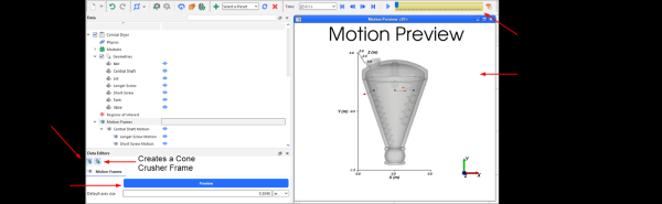 Figure 1: Motion Frames parameters in the Data Editors panel, and the Motion Preview window
* Motion Preview window works for all motions except for free body motions, which includes the ones created by the Cone
Crusher Frame
Figure 1: Motion Frames parameters in the Data Editors panel, and the Motion Preview window
* Motion Preview window works for all motions except for free body motions, which includes the ones created by the Cone
Crusher Frame
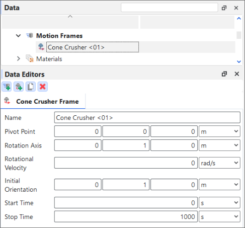
Table 1: Cone Crusher Frame parameters
Setting | Description | Range |
|---|---|---|
Name | Enables you to set a unique identifier for the selected frame. | 99 character limit |
Pivot Point | The coordinate location of the point around which the crusher and shaft will pivot, as specified in the X, Y, and Z directions. For first-level frames, this is based upon the global coordinate system. For nested or child frames, this is based upon the local coordinate system of the parent frame. | No limit |
Rotation Axis | The X, Y, and Z components that define the vector about which the crusher shaft and mantle are rotated. For first-level frames, this is based upon the global coordinate system. For nested or child frames, this is based upon the local coordinate system of the parent frame. | No limit but the values entered will be normalized |
Rotational Velocity | The angular velocity along the Rotation Axis. | No limit |
Initial Orientation | The X, Y, and Z components that define the vector about which the crusher shaft and mantle begin their rotation. | No limit but the values entered will be normalized |
Start Time | The time you want the crushing motion to begin. | Positive values |
Stop Time | The time you want the crushing motion to end. | Positive values |
What would you like to do?
From the Data panel, select Motion Frames.
From the Data Editors panel, ensure Default axes size is set the way you want, and then do one of the following:
To create a new parent Cone Crusher Frame, click the Create Cone Crusher Frame button. A new Cone Crusher entry appears under Motion Frames in the Data panel.
To create a new nested (child) Cone Crusher Frame, from the Data panel, select the parent Frame entry to which you want to add a child Cone Crusher Frame, and then from the Data Editors panel, click the Create Cone Crusher Frame button. A new Cone Crusher entry appears under the parent Frame you selected in the Data panel.
From the Data panel, select the Cone Crusher entry you just added and then from the Data Editors panel, enter the values you want. (See also About Creating and Applying Cone Crusher Frames to Imported Geometries.)
Tip: After creating a new Cone Crusher Frame, you must still apply the frame to your mantle and shaft geometries to have the geometries themselves move. (See also Apply a Cone Crusher Frame to Custom Mantle and Shaft Geometries.)
Note: Due to the free body motions involved, you cannot currently use the Motion Preview window to see and test the Cone Crusher Frames in 3D. (See also Preview a Motion in 3D.)
See Also:
Ensure the two geometries (mantle and shaft) to which you want to apply the Cone Crusher Frame have been imported.
Ensure the Cone Crusher Frame you want to apply has been created. (See also Create a Cone Crusher Frame.)
From the Data panel, select the imported mantle geometry to which you want to apply the Cone Crusher Frame.
From the Data Editors panel, select the Geometry tab, and then from the Motion Frame list, select the Cone Crusher Frame you want. (The Name will be appended with "Mantle".)
From the Data panel, select the imported shaft geometry to which you want to apply the Cone Crusher Frame.
From the Data Editors panel, select the Geometry tab, and then from the Motion Frame list, select the Cone Crusher Frame you want. (The Name will be appended with "Shaft".)
Note: Due to the free body motions involved, the Motion Preview window cannot currently preview these kinds of frames in 3D. (See also Preview a Motion in 3D.)
See Also:
From the Data panel, select Motion Frames.
From the Data Editors panel, ensure Default axes size is set the way you want, and then do one of the following:
To create a new parent Motion Frame, click the Create Motion Frame button. A new Frame entry appears under Motion Frames in the Data panel.
To create a new nested (child) Motion Frame, from the Data panel, select the parent Frame entry to which you want to add a child Motion Frame, and then from the Data Editors panel, click the Create Motion Frame button. A new Frame entry appears under the parent Frame you selected in the Data panel.
From the Data panel, select the Frame you just added and then from the Data Editors panel, do all of the following:
Enter the Name, Relative Position, Relative Rotation Vector, Rotation Angle, Keep in Place, and Periodic Motion values you want. (See also About Creating and Applying Motion Frames.)
Under Motions, click the Add Motion button, and enter the motion values you want. (See also Using Motion Frames to Create Specific Movements)
Repeat step 3b for every motion you want included within the new Motion Frame.
Tips:
After creating a new Motion Frame, you must still apply the Motion Frame to an imported geometry or Custom Input to have the component itself move. (See also Apply a Motion Frame to an Imported Geometry or Apply a Motion Frame to a Custom Input.)
After you have applied the Motion Frame to a geometry or Custom Input, you can use the Motion Preview window to see and test the movement in 3D. (See also Preview a Motion in 3D.)
See Also:
You can add Motion Frame to any geometry, wall or surface, created or imported into Rocky. An useful application is to add a Motion Frame to a surface that is attached to an Inlet or Outlet (See also About Adding and Editing Inlets and Outlets.) which allows for this inlet/outlet to be moved according to the Motion Frame. To apply a Motion Frame to a geometry do all of the following:
Ensure the Motion Frame you want to apply has been created. (See also Create a Motion Frame.)
From the Data panel, select the geometry to which you want to apply a Motion Frame.
From the Data Editors panel, select the Wall/Surface tab, and then from the Motion Frame list, select the Motion Frame you want.
Tips:
Use the Motion Preview window to see and test the movement in 3D. (See also Preview a Motion in 3D.)
To apply more than one movement to a single geometry, add multiple motions to a single Motion Frame, or create a nested (child) Motion Frame and then apply the child frame to the geometry. (See also Create a Motion Frame.)
See Also:
User processes created for post-processing, such as polyhedron (envelope), cubes and cylinders, can use motion frames to move around the domain and extract data while following geometries or particles.
Ensure the Motion Frame you want to apply has been created. (See also Create a Motion Frame.)
From the Data panel, select the User Process to which you want to apply a Motion Frame. (See also Filter Views and Data with User Processes.)
From the Data Editors panel, select the Polyhedron (Envelope)/Cube/Cylinder tab, and then from the Motion Frame list, select the Motion Frame you want.
Tip: To apply more than one movement to a single User Process, add multiple motions to a single Motion Frame, or create a nested (child) Motion Frame and then apply the child frame to the User Process. (See also Create a Motion Frame.)
See Also:
Ensure that the Particle Custom Inlet to which you want to apply a Motion Frame has been created. If the Particle set you assigned to the Input is a multi-element (flexible and/or discrete-breakable) Custom Fiber, at least one Segment should be defined as frozen. (This shape is also known as a frozen Fiber; see also About Adding and Editing Particle Inputs.) Important: All
releasetimes in the Particle Custom Inlet definition file must either be defined as 0 (zero) or thereleasefield itself must be omitted from the definition file.Ensure the Motion Frame you want to apply has been created. (See also Create a Motion Frame.)
From the Data panel, under Inputs, select the Particle Custom Inlet to which you want to apply a Motion Frame.
From the Data Editors panel, select the Particle Custom Inlets tab, and then from the Motion Frame list, select the Motion Frame you want.
Tips:
Even though you are able to use the Motion Preview window to see and test the movement in 3D, you will only be able to see the axes of the frame move and not the Custom Fibers. (See also Preview a Motion in 3D.)
To apply more than one movement to a single Particle Custom Inlet, add multiple motions to a single Motion Frame, or create a nested (child) Motion Frame and then apply the child frame to the Particle Custom Inlet. (See also Create a Motion Frame.)
See Also:
A Motion Preview Window is where you preview your motions to see how they affect the geometries in your simulation. Previewing is typically done after you have assigned the motion frame to the geometry but before you process the simulation.
Like other types of Rocky windows, you are able to define how the objects within the window and the window itself appears and function on screen. After you set up your Motion Preview window, you can choose to reuse the zoom, rotation, and pan settings in another window by saving and applying a Custom Camera Preset. You can also use the Motion Preview window as a basis for creating an animation of your motions.
What do you want to do?
See Also:
After you have defined one or more Motion Frames and have assigned them to your geometry components, a Motion Preview window is where you preview the geometry motions that you have defined. Previewing these motions before you process your simulation can allow you to catch and modify errors in your Motion Frame setup before particle calculations are introduced.
Notes:
In this version of Rocky, the Motion Preview window will preview the effects of gravity and any additional (prescribed) forces/moments that you have defined for free body motions, but will not be able to predict motions as a result of interactions with particles.
Even though you are able to preview the motion assigned to a Custom Input, only the axes for the frame will move; the particles themselves will not be visible in the preview.
Every Motion Frame with a free body motion defined must first be associated with a geometry component in order to preview it without error on the Motion Preview window.
After you set up your Motion Frames and apply them to the components you want to move (see also About Creating and Applying Motion Frames), you use the yellow-highlighted Time Toolbar to "play" the preview (Figure 1). (See also the Previewing Motions Using the Time Toolbar section in the About the Time Toolbar topic.)
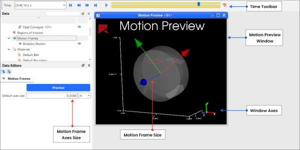
The length of the preview allowed by the Time Toolbar is based upon the Simulation Duration value you set in the Solver | Time tab (see also About Solver Parameters) with an upper limit of no more than 30,000 timesteps.
Within the Motion Preview window, each Motion Frame will be represented by its own set of axes. This axes set is tied to the local or parent coordinate of the frame and should not be confused with the set of window axes, which represents only the current orientation of the window itself. (See also About Using the Window Editors Panel to Change the Window Axes Displays.)
Tip: You can change the size of the Motion Frame axes through the Default Axes Size parameter. This is located on the Motion Frames tab of the main Motion Frames entity. (See also the Table 1: Motion Frames parameters (main entity) section in the About Creating and Applying Motion Frames topic.)
As with other windows in Rocky, there are various ways you can change what appears in a Motion Preview window, including fonts, overlays, background colors, and grid lines. If you want to share your motions outside of Rocky, you can also use the Motion Preview window as a basis for creating animations.
After a simulation is processed, Motion Preview windows are still viewable but not as useful for post processing as a 3D View window. This is because after a simulation is processed, both a 3D View and a Motion Preview window will show geometry movements, but only the 3D View window will also show particles. (See also About 3D View Windows.)
What do you want to do?
Notes:
In this version of Rocky, the Motion Preview window will preview the effects of gravity and any additional (prescribed) forces/moments that you define for free body motions, but will not be able to predict motions as a result of interactions with particles.
Even though you are able to preview the motion assigned to a Custom Input, only the axes for the frame will move; the particles themselves will not be visible in the preview.
Every Motion Frame with a free body motion defined must first be associated with a geometry component in order to preview it without error on the Motion Preview window.
Ensure that the motion you want to preview has been defined in a Motion Frame. (See also Create a Motion Frame).
Ensure that the geometry or Custom Input you want to move has been assigned the Motion Frame you want. (See also Apply a Motion Frame to an Imported Geometry or Apply a Motion Frame to a Custom Input.) Tip:Although you can preview a motion without first assigning it to a component, for geometries especially, it helps to see the movement if the Motion Frame is assigned to a geometry before previewing.
From the Data panel, select Motion Frames, and then from the Data Editors panel, click Preview. A new Motion Preview window appears in the Workspace.
Use the buttons on the Time toolbar (see also About the Time Toolbar) to play a preview of the motion as it might appear during the simulation. Tip:The Timestep slider turns yellow to indicate when it is being used to preview motion. If the Timestep slider is not yellow, it is being used to show simulated Timesteps as usual. Note: In preview mode, the Timestep slider is limited by the Simulation Duration value you set in the Solver | Time tab (see also About Solver Parameters) with an upper limit of no more than 30,000 timesteps.
Tips:
Zoom, pan, tilt, and fit the image just as you would in a 3D View window by using your mouse, keyboard, an/or the Camera Visualization toolbar. (See also Using the Mouse, Keyboard, or Toolbar to Change the View.)
Show/hide the individual Motion Frames you want previewed by using eye icons on the Data panel. (See also Show/Hide Components by Using Eye icons and Checkboxes.)
Change attributes of the geometries and motion objects shown within the window by using the Coloring tab. (See also About Using the Coloring Tab to Change the Motion Preview for a Frame.)
Change the attributes of the window itself, such as background colors, by using the Windows Editors panel. (See also About Using the Window Editors Panel to Change the Selected Motion Preview Window.)
For motions involving high frequency vibrations, ensure that you have set the Simulation Output Frequency (on the Solver | Time tab) low enough to properly preview the motion. (See also About Solver Parameters.)
See Also:
There are several ways you can change what you see in the Motion Preview window once you have created it, as explained below.
Zoom, pan, tilt, and fit the image by using your mouse, keyboard, and/or the Camera Visualization toolbar.
Change the colors and data attributes of the image, including the faces, edges, nodes, or vectors being displayed by using the Coloring tab on the Data Editors panel.
Show/hide the simulation entity you want displayed by using eye icons on the Data panel.
Change the attributes of the window itself, such as background colors, grid lines, and legend and caption details; and display options for the window axes by using the Window Editors panel.
You can also remove, rename, and show/hide a Motion Preview window just like any other window in Rocky.
What would you like to do?
See Also:
From the Window Editors panel, you can modify just the selected Motion Preview window to the change attributes including the background color, font color/sizes, and synchronize the Timesteps displayed when two or more view windows are open. You may also use the Window Editors panel to adjust the axes display settings for all the windows in your project.
What would you like to do?
When you use the Window Editors panel to change the selected Motion Preview window, you have the ability to change how items in the window appear on the screen. These items include background color, and font color/sizes (Figure 1). You can also change how multiple windows of the same type respond to changes in Timesteps.
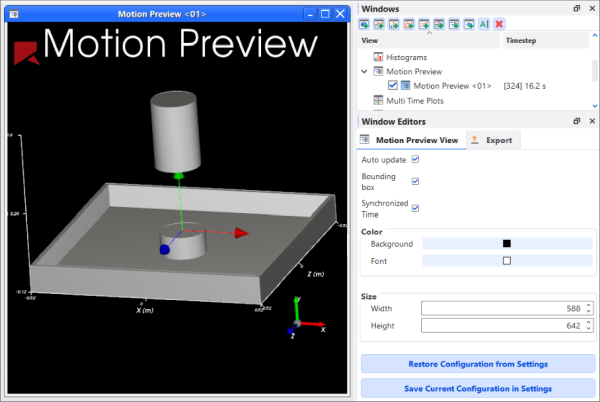
Tips:
You can also use Rocky Preferences to change the background color and fonts for all the Motion Preview windows in your project, instead of just the selected one. (See the "Preferences for Windows Properties" section in the About Setting Global Preferences topic.)
You can also change the window axes display for all windows in your project, including Motion Preview windows. (See also About Using the Window Editors Panel to Change the Window Axes Displays.) Note: The window axes is different from the motion frame axes, which has its own display settings. (See also About Creating and Applying Motion Frames.)
In this section, we will cover only the items on the Motion Preview View tab. Note: The Export tab will be covered in the About Exporting Data and Images Out of Rocky topic.
You use the Motion Preview View tab on the Window Editors panel to change how the window appears and how the data displayed within it is updated. These options include changing display items like the background color; labels, lines, and axes colors; color scale label sizes; and window height and width. In addition, you can choose to show or hide the Bounding box, which displays measurements illustrating the simulation boundaries; use Auto update to enable or prevent the view from being updated when data affecting it is changed; or choose to have multiple views updated with the same Timestep by using Synchronized Time.
See the image above and table below to understand more about how you can use the Window Editors panel to change a Motion Preview window.
Table 1: Motion Preview View tab options on the Window Editors panel
Setting | Description | Range |
|---|---|---|
Auto update | When enabled, any change made to the display settings of the selected Motion Preview window or to the items affecting the data or settings calculated and displayed within the Motion Preview, including the Timestep or Geometries displayed, will be updated in the Motion Preview window automatically. Because automatically updating the window with each separate change can be computationally intensive, you can clear this option to have all calculated items and more computationally intensive display options remain unchanged in the window until you enable Auto update again. Tip: You will know when the calculations in a Motion Preview window are not being updated when you see a thick red border around the window. | Turns on or off |
Bounding box | When enabled, displays measurements illustrating the simulation boundaries in the selected Motion Preview window. | Turns on or off |
Synchronized Time | When enabled and the window (or any other window with this checkbox enabled) is selected, the details shown in this (and any other Synchronized Time) window will be updated when the current Timestep is changed on the Time toolbar. (See also About the Time Toolbar.) When cleared and the window is selected, only this window will be updated when the current Timestep is changed on the Time toolbar. Tip: To keep the Timestep synchronized between multiple Motion Preview or other windows, ensure each window has this option enabled. | Turns on or off |
Color Background | Enables you to change the color that appears behind the geometries in the Motion Preview window. | Options limited by the choices in the Select Color dialog |
Color Font | Enables you to change the color of the labels, borders, and axes lines displayed in the Motion Preview window. | Options limited by the choices in the Select Color dialog |
Size Width | Enables you to numerically change how wide the selected window is. Useful in cases where you need exact dimensions for image consistency, or when generating animations. | Whole positive values between 123 and 5000. |
Size Height | Enables you to numerically change how tall the window is. Useful in cases where you need exact dimensions for image consistency, or when generating animations. | Whole positive values between 0 (zero) and 5000. |
Restore Configuration from Settings | Clicking this button replaces the values set on the tab with the ones that have been saved to the (internal) Rocky Settings folder. (See also Rocky File Types and Folders.) | (Button selection) |
Save Current Configuration in Settings | Clicking this button overwrites the values that have been saved to the (internal) Rocky Settings folder with the ones currently set on the tab. (See also Rocky File Types and Folders.) | (Button selection) |
What would you like to do?
See Also:
Ensure the Window Editors panel is visible. (From the View menu, click Window Editors.)
From the Workspace, select the Motion Preview window that you want to change. (See also Preview a Motion in 3D.)
From the Window Editors panel, select the Motion Preview View tab and then change the options you want.
Tips:
You can also open the Window Editors panel for a window by right-clicking an empty space within the Motion Preview window (for example, the background behind the geometries), and then clicking Settings.
You can also use Rocky Preferences to change the background color and fonts for all the Motion Preview windows in your project, not just selected one. (See the "Preferences for Windows Properties" section in the About Setting Global Preferences topic.)
To reuse in future projects the settings you made to this tab, click the Save Current Configuration in Settings button.
To apply settings you have already saved (either by previously using the Save Current Configuration in Settings button or by saving selections within the Preferences dialog) to this tab, click the Restore Configuration from Settings button.
See Also:
The Coloring tab, which is located on the Data Editors panel for all simulation entities and User Processes, enables you to change the image of the items being displayed within your Motion Preview window. These include the geometry components and any user processes created from those geometry components. It also includes individual Motion Frames whose Coloring tab shows options related to the axes of the Frame that is selected in the Data panel.
What would you like to do?
See Also:
Using the options on the Coloring tab is one way you can change the appearance of the items being displayed in a Motion Preview window. Visualization options for the Faces, Edges, and Nodes can be modified with the Coloring tab for any of the following entities:
Inlets
Any User Process created from any of the above entities
In addition, when an individual Motion Frame is selected in the Data panel, the Coloring tab for that entity shows options related to the axes of the selected Frame (Figure 1).
See the images and tables below to help you understand how to use the Coloring tab to change a view for selected entity.
Figure 3.123: Coloring tab when a Motion Frame is selected in the Data panel AND a Motion Preview window is selected
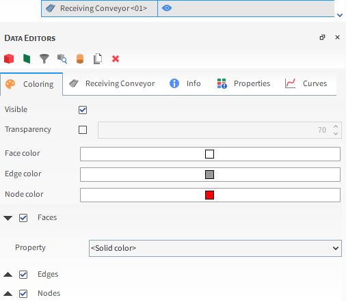
Table 1: Coloring tab parameter options for a Motion Frame when a Motion Preview window is selected
Setting | Description | Range |
|---|---|---|
Visible | When enabled, shows the selected entity in the active view window. Note: This is the same as using the Data panel eye icon. (See also Show/Hide Components by Using Eye icons and Checkboxes.) | Turns on or off |
Inherit Axes Size? | When enabled, allows the selected Frame to use the same axes size as what was set in the main Motion Frames entity (see also About Creating and Applying Motion Frames to Imported Geometries). When cleared, enables you to set a unique axes size for the selected Motion Frame. | Turns on or off |
Axes Size | When the Inherit Axes Size? checkbox is cleared, this defines the custom axes size for the selected Frame. | Positive value |
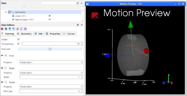
Table 2: Coloring tab parameter options for a geometry component when a Motion Preview window is selected
Setting | Description | Range |
|---|---|---|
Visible | When enabled, shows the selected entity in the active view window. Note: This is the same as using the Data panel eye icon. (See also Show/Hide Components by Using Eye icons and Checkboxes.) | Turns on or off |
Transparency | Enables boundaries to be drawn transparently in the selected view window. A value of 0 (zero) makes the faces completely solid or opaque. A value of 100 makes the faces completely transparent or hidden. | Turns on or off; 0-100 |
Color | When Faces, Edges, and/or Nodes are selected and the Property is <Solid Color>, this enables the selected display type to be colored in the one solid color chosen. Note: For Faces, Transparency options affect how opaque this color appears in the view. | Options limited by the Select Color dialog |
Faces | Enables the entire surface of the entity to be visible and affected by the various Faces coloring options. | Turns on or off |
Property | Three separate lists under Faces, Edges, and Nodes respectively provide properties and other color options that apply to the display type within which the list is contained. Specifically:
| <Solid color>; List of properties automatically generated from the Properties tab |
Show on Node? | When Faces is enabled and a property is selected from the Property list under Faces, this enables the visualization of the selected property to be evenly interpolated across the entity for a smoother visualization. | Turns on or off |
Edges | Enables only the edges bordering the components making up the entity boundaries visible and affected by the various Edges coloring options. | Turns on or off |
Width | When Edges is selected, this changes the thickness of the lines used to draw the borders. Entering 1 will provide the narrowest line. | Positive values |
Nodes | Enables the points marking the intersections of the entity's individual components to be visualized as dots and affected by the various Nodes coloring options. | Turns on or off |
Point Size | When Nodes is selected, this changes the size of the dots used to draw the nodes. Entering 1 will provide the smallest dot. | Positive values |
What would you like to do?
See Also:
From the Workspace, select the Motion Preview window to which you want to apply changes. (See also Preview a Motion in 3D.)
From the Data panel, do one of the following:
Under Geometries, select the geometry component or inlet that you want to change.
Under Motion Frame, select the Frame you want to change.
From the Data Editors panel, select the Coloring tab, and then change the settings that you want. The changes you make are shown automatically in the Motion Preview window.
See Also:
Once you know how to create and apply Motion Frames to an imported geometry (see also About Creating and Applying Motion Frames to Imported Geometries), there are many different types of movements you can create. Use this section to learn more about how to create some specific movements for your geometries.
What would you like to do?
Use Motion Frames to Enable a Regularly Swinging Boundary (e.g. a Pendulum)
Use Motion Frames to Enable a Geometry to Freely Move Linearly
Use Motion Frames to Enable a Geometry to Freely Move Linearly with an Added Force
Use Motion Frames to Enable a Geometry to Freely Rotate Around its Center Point
Use a Cone Crusher Frame to Enable a Geometry to Adopt a Crushing Motion
Use Motion Frames to Enable Multiple Movements of a Geometry in one Simulation
Ensure the geometry you want to move has already been imported.
Create a Motion Frame as you normally would (see also Create a Motion Frame), but under Motions (step 3b), ensure that you do all of the following:
Determine when you want the motion to start and stop by entering the values you want for Start Time and Stop Time.
From the Type list, select Translation.
From the Input list, do one of the following:
To set only a fixed velocity with no acceleration, select Fixed Velocity, and then enter the Velocity you want in the X, Y, and Z axes respectively.
To set both the initial and final velocity and have Rocky compute the acceleration required to achieve those values, select Initial and Final Velocity and then enter the Initial Velocity and Final Velocity you want in the X, Y, and Z axes respectively.
To set both the initial velocity and the acceleration values and then have Rocky compute the final velocity that results from those values, select Initial Velocity and Acceleration and then enter the Initial Velocity and Acceleration values you want in the X, Y, and Z axes respectively.
Apply the new Motion Frame to the geometry you want to move. (See also Apply a Motion Frame to an Imported Geometry.)
Use the Motion Preview window to see and test the movement in 3D. (See also Preview a Motion in 3D.)
See Also:
Ensure the geometry you want to move has already been imported.
Create a Motion Frame as you normally would (see also Create a Motion Frame), but ensure that you do all of the following:
For Relative Position, enter the location of the geometry's center point.
Under Motions (step 3b), do all of the following:
Determine when you want the motion to start and stop by entering the values you want for Start Time and Stop Time.
From the Type list, select Rotation.
Enter the Initial Angular Velocity you want in the X, Y, and Z axes respectively.
If you want velocity affected by acceleration, enter the Angular Acceleration you want in the X, Y, and Z axes respectively.
Apply the new Motion Frame to the geometry you want to move. (See also Apply a Motion Frame to an Imported Geometry.)
Use the Motion Preview window to see and test the movement in 3D. (See also Preview a Motion in 3D.)
See Also:
Note: Use this procedure when the swinging motion is applied to the geometry in a predictable and regular manner. To enable a boundary that swings freely based upon particles acting upon it, see the procedure Use Motion Frames to Enable a Geometry to Rotate Freely Around a Non-Center Point (e.g., a Gate or Rubber Curtain).
Ensure the geometry you want to move has already been imported.
Create a Motion Frame as you normally would (see also Create a Motion Frame), but under Motions (step 3b), ensure that you do all of the following:
Determine when you want the motion to start and stop by entering the values you want for Start Time and Stop Time.
From the Type list, select Periodic Rotation (Pendulum).
Enter the Initial Frequency and Initial Amplitude.
For Direction, enter the X, Y, Z vector components defining the 2D plane upon which the swinging will occur.
For Initial Phase, enter the starting angular degree (Plane Angle) you want to use.
If you want the frequency or amplitude to vary per unit of time for the selected motion, enter what you want for Frequency Variation and Amplitude Variation.
Apply the new Motion Frame to the geometry you want to move. (See also Apply a Motion Frame to an Imported Geometry.)
Use the Motion Preview window to see and test the movement in 3D. (See also Preview a Motion in 3D.)
See Also:
Ensure the geometry you want to move has already been imported.
Create a Motion Frame as you normally would (see also Create a Motion Frame), but under Motions (step 3b), ensure that you do all of the following:
Determine when you want the motion to start and stop by entering the values you want for Start Time and Stop Time.
From the Type list, select Periodic Translation (Vibration).
Enter the Initial Frequency and Initial Amplitude.
For Direction, enter the X, Y, Z vector components defining the direction over which the vibrating motion will occur.
For Initial Phase, enter the starting angular degree (Plane Angle) you want to use.
If you want the frequency or amplitude to vary per unit of time for the selected motion, enter what you want for Frequency Variation and Amplitude Variation.
Apply the new Motion Frame to the geometry you want to move. (See also Apply a Motion Frame to an Imported Geometry.)
Use the Motion Preview window to see and test the movement in 3D. (See also Preview a Motion in 3D.) Tip:For motions involving high frequency vibrations, ensure that you have set your Solver | Output Frequency low enough to properly preview the motion. (See also About Solver Parameters.)
See Also:
Ensure the geometry you want to move has already been imported.
Create a Motion Frame as you normally would (see also Create a Motion Frame), but under Motions (step 3b), ensure that you do all of the following:
Determine when you want the motion to start and stop by entering the values you want for Start Time and Stop Time.
From the Type list, select Free Body Translation.
From the Free Motion Direction list, select the axis or axes that you want free motion enabled. Tip:To have Free Motion enabled in every possible direction, select All directions.
Apply the new Motion Frame to the geometry you want to move. (See also Apply a Motion Frame to an Imported Geometry.) Note: With free body motions, missing this step will result in errors when you later try to either preview the motion or process the simulation.
Use the Motion Preview window to see and test the effects of gravity. (See also Preview a Motion in 3D.)
Note: Because the movement of a geometry with Free Motion is directly affected by particle interactions yet to be calculated, the Motion Preview window will only be able to preview the effects of gravity and any additional (prescribed) forces/moments you have defined.
See Also:
Ensure the geometry you want to move has already been imported.
Create a Motion Frame with a Free Body Translation Motion Type. (See also Use Motion Frames to Enable a Geometry to Freely Move Linearly.)
Add a second Motion to the selected Frame by clicking the Add Motion button, and then do all of the following:
Determine when you want the motion to start and stop by entering the values you want for Start Time and Stop Time.
From the Type list, select Additional Force.
For Force Value, enter the X, Y, and Z components defining the amount of additional, applied force you want acted upon the selected Frame.
#. Apply the new Motion Frame to the geometry you want to move. (See also Apply a Motion Frame to an Imported Geometry.) Note: With free body motions, missing this step will result in errors when you later try to either preview the motion or process the simulation. #. Use the Motion Preview window to see and test the effects of gravity and the additional (prescribed) forces/moments that you defined. (See also Preview a Motion in 3D.)
Note: Because the movement of a geometry with Free Motion is directly affected by particle interactions yet to be calculated, the Motion Preview window will only be able to preview the effects of gravity and any additional (prescribed) forces/moments that you have defined.
See Also:
Ensure the geometry you want to move has already been imported.
Create a Motion Frame as you normally would (see also Create a Motion Frame), but ensure that you do all of the following:
For Relative Position, enter the location of the geometry's center point.
Under Motions (step 3b), do all of the following:
Determine when you want the motion to start and stop by entering the values you want for Start Time and Stop Time.
From the Type list, select Free Body Rotation.
From the Free Motion Direction list, select the axis or axes that you want free motion enabled. Tip:To have Free Motion enabled in every possible direction, select All directions.
Apply the new Motion Frame to the geometry you want to move. (See also Apply a Motion Frame to an Imported Geometry.) Note: With free body motions, missing this step will result in errors when you later try to either preview the motion or process the simulation.
Use the Motion Preview window to see and test the effects of gravity. (See also Preview a Motion in 3D.)
Note: Because the movement of a geometry with Free Motion is directly affected by particle interactions yet to be calculated, the Motion Preview window will only be able to preview the effects of gravity and any additional (prescribed) forces/moments you have defined.
See Also:
Ensure the geometry you want to move has already been imported.
Create a Motion Frame with a Free Body Rotation Motion Type (see also Use Motion Frames to Enable a Geometry to Freely Rotate Around its Center Point) but be sure to set the Frame Relative Position to be the coordinate location of the point you want the geometry to rotate around.
Add a second Motion to the selected Frame by clicking the Add Motion button, and then do all of the following:
Determine when you want the motion to start and stop by entering the values you want for Start Time and Stop Time.
From the Type list, select Additional Moment.
For Moment Value, enter the X, Y, and Z components defining the amount of additional, applied moment (torque) you want acted upon the selected Frame.
Apply the new Motion Frame to the geometry you want to move. (See also Apply a Motion Frame to an Imported Geometry.) Note: With free body motions, missing this step will result in errors when you later try to either preview the motion or process the simulation.
Use the Motion Preview window to see and test the effects of gravity and the additional (prescribed) forces/moments that you defined. (See also Preview a Motion in 3D.)
Note: Because the movement of a geometry with Free Motion is directly affected by particle interactions yet to be calculated, the Motion Preview window will only be able to preview the effects of gravity and any additional (prescribed) forces/moments that you have defined.
See Also:
Ensure that both the mantle and shaft geometries you want to move have already been imported.
Create a Cone Crusher Frame as you normally would (see also Create a Cone Crusher Frame).
Apply the new Cone Crusher Frame to the two geometries you want to move. (See also Apply a Cone Crusher Frame to Custom Mantle and Shaft Geometries.)
Note: Due to the free body motions involved, you cannot currently use the Motion Preview window to see and test the Cone Crusher Frames in 3D. (See also Preview a Motion in 3D.)
See Also:
Ensure the geometry you want to move has already been imported.
Create a Motion Frame as you normally would (see also Create a Motion Frame).
Do one of the following:
To create an additional motion within the selected Motion Frame, click the Add Motion button, and set up the additional motion as you normally would.
To create a separate Frame linked to the selected Motion Frame, do the following:
Click the Add Motion Frame button. A nested (child) Frame appears beneath the original Frame in the Data panel.
From the Data panel, select the new Frame, and then set up the motion as you normally would.
Apply the Motion Frame to the geometry you want to move. (See also Apply a Motion Frame to an Imported Geometry.) Specifically:
For multiple motions within one Motion Frame, apply the single Motion Frame to the geometry. All motions within the Motion Frame will be applied.
For multiple nested Motion Frames, apply the lowest-level child Motion Frame to the geometry. All Motion Frames linked to the child, including their defined motions, will be applied.
Use the Motion Preview window to see and test the movement in 3D. (See also Preview a Motion in 3D.)
See Also:
Ensure the geometry you want to have periodic motions has already been imported.
Create a Motion Frame as you normally would (see also Create a Motion Frame), but but for part 3a, do the following:
Be sure that you enable the Enable Periodic Motion checkbox.
In the Periodic Start Time box, enter the amount of delay after the motion(s) Start Time and Stop Time to begin and end the motion to be repeated.
In the Periodic Stop Time box, enter the exact time you want the motion(s) to stop, regardless of what is set for its Stop Time.
Tip: To ensure that the periodic motion continues for the entire simulation, keep this value set to the default (1000 s) or set it higher than your simulation duration.
In the Period box, enter how much of the original motion(s) will be repeated.
Continue setting up your Motion Frame as you normally would.
Use the Motion Preview window to see and test the movement in 3D. (See also Preview a Motion in 3D.)
Tips:
To have the periodic motion appear at simulation onset, keep both the Start Time and Periodic Start Time zero (0).
See Also:
Rocky enables you to specify unique properties for both solid and fluid materials. Conveyor belts, geometries, and particle sets and fluid elements used in your simulation can each have specific materials, allowing you to ensure that the various components being simulated interact with each other in as realistic a way as possible.
What would you like to do?
See Also:
By default, Rocky defines three Solid Material sets for each simulation (for Default Belt, Default Boundary and Default Particle). While you can modify the settings for these default Materials and also add additional Material definitions if you choose, you cannot remove them from the simulation.
Materials you define here will be used when defining the parameters for Geometries, Particles, and Materials Interactions.
If you have enabled one or more external Modules that affect your Materials settings, you might also have separate, module-specific settings that you can define. Refer to the Module's documentation (if provided) for more information. (See also Rocky Simulation Entities that can be Affected by Modules.)
Use the figures and table below to help you understand the various parameters you can modify for Materials.
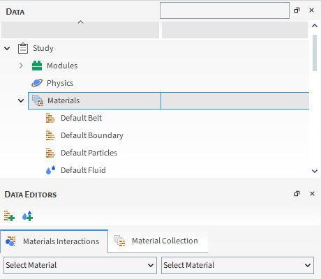
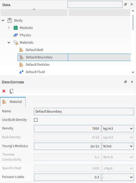
Table 1: Material parameter options (all available)
Setting | Description | Range |
|---|---|---|
Bulk Solid Fraction for Materials | For all Materials that have the Use Bulk Density checkbox enabled, this number is applied to the (disabled) Density value of the Material. For all Materials that have the Use Bulk Density checkbox cleared, this number is applied to the (disabled) Bulk Density of the value. Notes:
| 0<1 |
Name | Enables you to specify a unique identifier for the Material. | 99 character limit |
Use Bulk Density | When selected, the Density of the particles will be calculated using both the Bulk Density and the Bulk Solids Fraction for Materials values. When cleared, the Density value you enter directly will be used instead. Note: No matter what you choose here, only the Density value-either entered directly by you or calculated by Rocky (and shown grayed-out) based upon the bulk density values you provided-is used for DEM calculations. | Turns on or off |
Density | The particle density or true density of a particulate solid or powder is the density of the material that makes up the particles. No matter whether this value is entered by you or is calculated by Rocky (and shown grayed- out) based upon the bulk density values you provided, only this value will be used for DEM calculations. | Positive values |
Bulk Density | The bulk density or apparent density of a material is defined as the mass of particles divided by the total volume they occupy. The total volume includes particle volume, inter-particle void volume, and internal pore volume. Therefore, bulk density is not an intrinsic property of a material; it can change depending upon how the material is handled and compacted; i.e., it depends upon the Bulk Solid Fraction. For example, a powder poured into a cylinder will have a particular bulk density; if the powder is then compacted by the application of a certain force over the particles, particles will move and stay closer together, resulting in a higher bulk density. Bulk density of granular materials is usually reported both as "freely settled" (or "poured" density) and "tapped" density, which is the bulk density of the material after a specified compaction process. | Positive values |
Young's Modulus | A measure of the capacity of a material to withstand changes in length when under lengthwise tension or compression. Defines the relationship between force per unit area and proportional deformation, and is assigned as separate values to each particle and boundary material defined. Applied in contact stiffness calculations used in the models for normal and tangential forces for each pair of particle-to-particle or particle-to-boundary collisions. In general, the higher the value, the more accurate the results but the longer the processing time. | Positive values |
Thermal Conductivity | When Thermal Model is enabled (see also About Physics Parameters), this sets the thermal conductivity value for the material. | Any value |
Specific Heat | When Thermal Model is enabled (see also About Physics Parameters), this sets the specific heat value for the material. | Any value |
Poisson's Ratio | This sets the Poisson's Ratio value for the material. Note: Even though you are always able to set this parameter, it will only be used in the following scenarios:
| Any value Tip: Most materials will have a Poisson's Ratio value ranging between 0.0 and 0.5 |
See Also:
By default, Rocky defines a Fluid Material. While you can modify the settings for this default Material and also add additional Material definitions if you choose, you cannot remove it from the simulation.
Materials you define here will be used when defining the parameters for the Fluid phase, and its interactions.
If you have enabled one or more external Modules that affect your Materials settings, you might also have separate, module-specific settings that you can define. Refer to the Module's documentation (if provided) for more information. (See also Rocky Simulation Entities that can be Affected by Modules.)
Use the figures and table below to help you understand the various parameters you can modify for Fluid Materials.
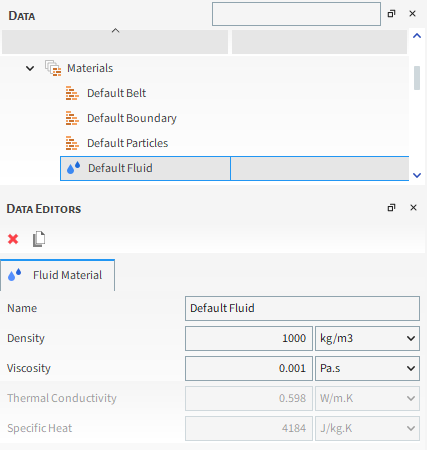
Table 1: Fluid material parameter options
Setting | Description | Range |
|---|---|---|
Name | Enables you to specify a unique identifier for the Material. | 99 character limit |
Density | The initial density of the SPH elements which is used in the equation of state to compute the relation between pressure and density. | Positive values |
Viscosity | Defines the fluid material dynamic viscosity. | Positive values |
Thermal Conductivity | When Thermal Model is enabled (see also About Physics Parameters), this sets the thermal conductivity value for the material. | Any value |
Specific Heat | When Thermal Model is enabled (see also About Physics Parameters), this sets the specific heat value for the material. | Any value |
Sound Speed* | Parameter used in the equation of state to compute the relation between pressure and density. It also defines the SPH solver timestep. | Positive values |
*While low sound speed can leed to numerical instabilities, high sound speeds increase the simulation cost due to the smaller time step. Refer to SPH technical manual for guidelines on selecting the material sound speed.
See Also:
Rocky enables you to specify unique frictions and adhesion values for each Material-to-Material combination that exists in your simulation, including the interaction of a Material to itself, and also to each other Material defined in the Materials list.
Modifying Materials Interactions values enables you to calibrate how "wet" or "sticky" a Material acts when it comes into contact with another Material, enabling you to create simulations that more closely mirror real-world conditions.
Tip: It is good practice to calibrate your particle settings to the real-world behavior of the material you are simulating before changing your materials interaction settings. You may wish to use the Material Wizard and/or the Calibration Suite to help you with this task.
While the Adhesive Force models used for these interaction settings are defined as part of the Set Simulation-Wide Parameters step (see also About Physics Parameters), and the characteristics of the individual Materials are defined in the Modifying Material Compositions step (see also About Modifying Material Compositions, the purpose of this step is to define specific material-to-material parameters. These can include parameters for Momentum, Adhesion, and Restitution.
Important: Even though Rocky enables you to set interactions of geometries to other geometries, these types of interactions have no value to your simulation. The only values that will affect your simulation are those interactions between particles (particle-to-particle) or between particles and boundaries (particle-to-geometry).
If you have enabled one or more external Modules that affect your Materials Interactions settings, you might also have separate, module-specific settings that you can define. Refer to the Module's documentation (if provided) for more information. (See also Rocky Simulation Entities that can be Affected by Modules.)
Use the figure and table below to help you understand the various parameters you can modify for Materials Interactions.
Figure 3.128: Materials Interactions parameters in the Data Editors panel for a Constant Adhesive Force
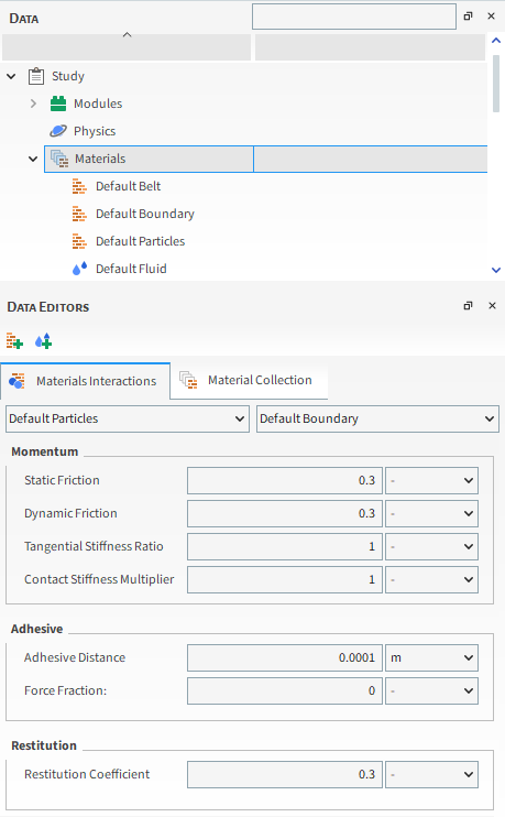
Table 1: Materials Interactions parameter options
|
Setting Momentum |
Description |
Range |
|
Static Friction |
Maximum ratio of contact tangential force to normal force before onset of sliding. |
Positive values (see also Best Practices for Setting Up Particles) |
|
Dynamic Friction |
Maximum ratio of contact tangential force to normal force after onset of sliding. |
Positive values; usually less than Static Friction (see also Best Practices for Setting Up Particles) |
|
Tangential Stiffness Ratio |
When the Linear Spring Coulomb Limit model is selected for Tangential Force (see also About Physics Parameters), this defines the ratio of tangential contact stiffness to normal contact stiffness. This parameter controls the bulk Poisson's ratio of granular materials. Tip: If knowing the exact relationship between this value and the resulting bulk Poisson's ratio is required, calibration is recommended. This is due to the fact that in addition to this value, other factors including size distribution and friction parameters affect the final bulk Poisson's ratio amount. |
0-1 Tip: It is recommended that 1 be used for most simulations. |
|
Contact Stiffness Multiplier |
When the Advanced Features checkbox is enabled on the Additional Features tab of the Options | Preferences dialog (see also About Setting Global Preferences), this enables you to keep (value = 1) or increase (value > 1) the effect of stiffness upon the selected pair of materials when they come into contact during the simulation. Increasing the contact stiffness can help decrease the particle overlap, and is accomplished by multiplying this value by the contact stiffness that Rocky calculates. Tip: To learn more about how Rocky calculates Contact Stiffness, refer to the DEM Technical Manual. (From the Rocky Help menu, point to Manuals and then select DEM Technical Manual.) Note: This text field does not support parametric variables. (See also I cannot enter an input variable or mathematical function into a text field) |
1 or greater |
|
Adhesive | ||
|
Adhesive Distance |
When a Constant or Linear Adhesive Force is chosen, this is the distance between the two Materials before forces are applied. |
Positive values |
|
Force fraction |
When a Constant Adhesive Force is chosen, this is the ratio of the adhesive force on the first Material to the gravity force of the second Material. |
Positive values |
|
Stiffness fraction |
When a Linear Adhesive Force is chosen, this is the ratio of adhesive stiffness to the loading elastic stiffness of the contact between the two materials. |
0-1 |
|
Surface Energy |
When a JKR Adhesive Force is chosen, this sets what Surface Energy will be used. For more information about these models, see the Rocky Technical Manual. (From the Rocky program Help menu, point to Manuals, and then click DEM Technical Manual.) |
Positive values |
|
Restitution | ||
|
Restitution Coefficient |
Measure of energy dissipation. |
Greater than 0 (zero) but less than or equal to 1 Note: The recommended range is 0.1 - 1.0 |
|
Velocity Limit |
When the Experimental (Beta) Features checkbox is enabled on the Options | Preferences dialog (see also About Setting Global Preferences) and Velocity Dependent is selected for Restitution Model (see also About Physics Parameters), this is the velocity limit for the restitution. |
Values above 10e-5 |
|
Velocity Exponent |
When the Experimental (Beta) Features checkbox is enabled on the Options | Preferences dialog (see also About Setting Global Preferences) and Velocity Dependent is selected for Restitution Model (see also About Physics Parameters), this is the velocity exponent for the restitution. |
Any value |
|
Other "Modules" Settings | ||
|
(Varies) |
These settings are specific to only certain external Module and are therefore not documented in the Rocky User Manual. Refer to the Module's documentation (if provided) for more information. (See also Rocky Simulation Entities that can be Affected by Modules) |
(Varies) |
What would you like to do?
See Also:
Ensure that you have set the Adhesive Force parameters you want as part of the Set Simulation-Wide Parameters step. (See also About Physics Parameters.)
Ensure that you have set the Materials you want and have defined their compositions. (See also About Modifying Material Compositions.)
From the Data panel, select Materials. The Materials Interactions parameters become active in the Data Editors panel.
From the Data Editors panel, do all of the following:
From Select Material list on the left, select the first Material in the Material-to-Material combination for which you want to modify interaction values.
From the Select Materials list on the right, select the next Material in the Material-to-Material combination for which you want to modify interaction values. The parameters that define the interaction between the two Materials you selected appear in the Data Editors panel.
Modify the values as you want.
Repeat steps 3a-3c for each of the Material-to-Material combinations you want to modify.
See Also:
A Particle set is created when you specify the shape of a particular particle, and then choose the size ranges (and, if desired, the breakage parameters) you want replicated in your simulation.
Particle sets are a subset of the Particles entity, which contain the Properties and Curves for your Particle set(s). You can preview Particle shapes in a Particles Details window, and if you have collected collision statistics during processing, can use that same window to view the results on a representative particle.
See Also:
You can add as many unique Particle sets containing as many size ranges each to a given simulation as you like, but you must have added at least one Particle set and one Particle Input to process a simulation.
See the sections below for details on the various settings you can assign to a particle set.
On the main Particle tab (Figure 1), the Shape you choose for your Particle set largely determines what models and settings can be applied thereafter.
Shape attributes such as whether your particle is spherical or shaped; has sharp corners or rounded corners; made of three-, two-, or one-dimensional components; is convex or concave; and so on, affect whether a particle can be divided (or meshed) into various Elements, made to be flexible, have calculations such as breakage or thermal applied to them, and more.
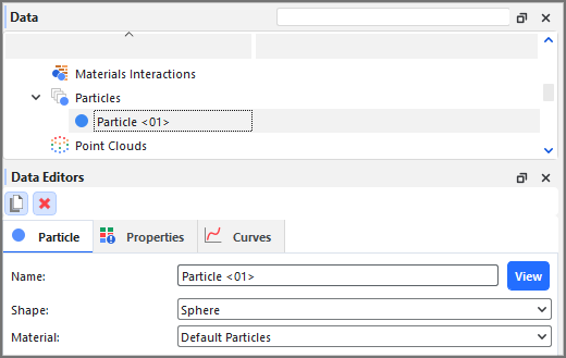
There are currently four categories of particle shapes that can be used in Rocky:
Fiber particles, which are strand-like 3D objects made by stringing together linear Segments and where each segment can have its own thickness. This thickness along with the sieve size (see the Size Tab section below) helps determine the number of elements used to make up the shape (see the Composition Tab section below). Rocky comes with a Straight Fiber by default (Table 1), but other Custom Fiber shapes (Table 2) can be imported with a text or spreadsheet file. (To learn more about creating a Custom Fiber definition file, see About Defining and Importing Custom Particle Shapes.)
Shell particles, which are sheet- or container-like 3D objects made by joining two-dimensional, open surfaces of a definable thickness. Because they contain no interior volume, the mass of a Shell particle is much lower than a similarly shaped Solid particle. Similar to a Custom Fiber shape, you can determine the thickness of the surfaces that make up the Shell shape which, along with sieve size, affect the mass and the number of elements Rocky will use to make up the shape (see the Composition Tab section below). No default Shell particles come with Rocky, but you can add your own Custom Shell shapes (Table 2) by importing an .stl file.
Solid particles, which are closed 3D objects of full interior volume. Seven Solid shapes are provided by default (Table 1), and you can also import your own Custom Polyhedron shape (Table 2) from an .stl file. (See also About Defining and Importing Custom Particle Shapes.)
Assembly particles, which are made by combining the shape of other Particles sets together into a single, unique particle (Table 3). When compared to importing a similar custom .stl shape, an Assembly particle has the ability to run much faster due to simpler calculations, especially when multiple convex shapes are assembled to represent a concave shape.
Note: Different shapes types have different capabilities in Rocky. Refer to Rocky Particle Shapes and Capabilities for specifics.
Table 1: Default shape types in Rocky
Default Spherical (Solid) | Default Fiber | |
|---|---|---|
|
|
|
|
|
|
|
|
|
|
|
|
|
|
|
|
|
|


Table 2: Example custom (imported) shape types
Custom Polyhedron (Solid) | Custom Shell | Custom Fiber |
|---|---|---|
Note: If any portion of a Custom Polyhedron is concave, no matter how small a portion, Rocky considers the whole shape to be concave. |
|
|

Table 3: Example Assembly shape types
Using Only Default (Solid) Shapes | Using Solid and Straight Fiber Shapes | Using Custom Imported Convex Shapes |
|---|---|---|
|
|
|


(See also About Particle Assemblies.)
You can review the shape you select (or import) from the Shape list by choosing to see a View (Figure 2) of the particle shape, which opens in its own window called a Particles Details window. (See also About Particles Details Windows).

In this version, the preview reflects the size of the largest particle in the selected Particle set. (See Size Tab section below for more information.)
Notes:
The Particles Details window can also be used to display collision statistics for certain particle shapes after processing. (See also About Intra-Particle Collision Statistics.)
For Assembly shapes, the Particles Details 3D view shows the actual position of the part when the size type is Original Size Scale, and it is set to 1 (which is the default setting).
The Geometric Center for an Assembly particle is represented in the Particles Details window as a yellow dot, and the Center of Mass is represented by a blue dot.
You can modify some of the default shapes that come with Rocky by adjusting the attributes-such as the vertical and horizontal aspects, and number of corners-on the Shape sub-tab (Figure 3).
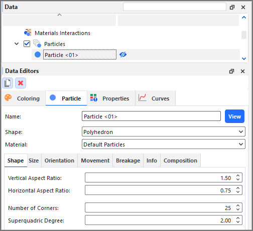
In this way, you can derive a wide variety of different real-particle shapes. (See also Appendix A: Particle Shape Examples.)
If you are creating an Assembly shape, you will have different options on the Shape tab (Figure 4). These options enable you to choose which individual particles' shapes (parts) will make up the final assembled shape, and how those parts are presented (locations, sizes, rotations) in the Assembly. (See also About Particle Assemblies.)
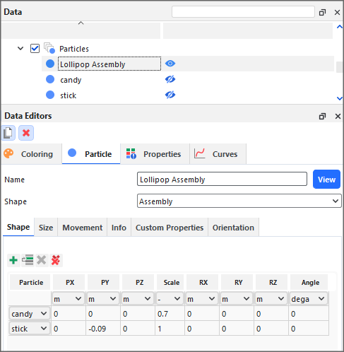
After importing your Custom Polyhedron shape, you will be able to use the options on the Shape tab to select a different STL file (Figure 5).
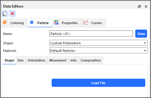
When importing a Custom Shell particle shape, Rocky assigns an initial (and arbitrary) thickness value during import. This value is reflected in the Particles Details window when 100% Original Size Scale is selected on the Size tab. (See Size Tab section below.) The Shape tab will then allow you to enter a new Thickness value so that you may achieve the desired thickness of your imported particle shape (Figure 6).
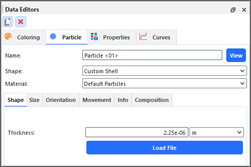
The Thickness value that is entered here represents the actual thickness of the largest particle in the set at 100% of its imported size, taking into account any scaling that you have indicated on the Import File Info dialog. Halving the Thickness value will reduce the relative thickness of all particles in your set by 50%; doubling the value will increase the relative thickness 200%, and so on.
Once you have set up your particle shape to your liking, you can then choose to export it to an .stl file for further analysis outside of Rocky. (See also Export a Particle Shape to an STL File.)
The Size tab (Figure 7) is where you define the Particle Size Distribution (PSD) of your Particle set, and the method by which the particle size will be measured.
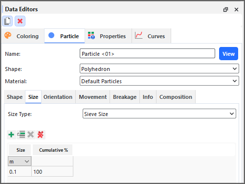
In this version of Rocky, there are three different methods, or **Size Type**s, by which you can define your particle sizes:
Sieve Size (formerly "Sieve"), which for especially default Rocky shapes, bases particle size upon a virtual mesh
hole just big enough for the particle to pass through. Note: Due to the way Sieve Size is calculated, it should be used only for even and balanced particle shapes (such as the default Solid particles included with Rocky) and not for fibers or shapes with high aspect ratios. (For more detail on how Sieve Size is calculated in Rocky, see the DEM Technical Manual. (From the Rocky Help menu, point to Manuals, and then click DEM Technical Manual.)) - Equivalent Sphere Diameter (formerly "Equivalent Diameter"), which for especially irregular objects, bases particle size upon the diameter of a sphere with equivalent volume. Tip:To see a walk-through example of setting and using Equivalent Sphere Diameter, refer to the following Workshop: Tutorial - Windshifter in the Rocky Tutorial Guide. - Original Size Scale, which for especially imported and Assembly shapes, bases particle size upon the original size of the shape. Tip:To see a walk-through example of setting and using Original Size Scale, refer to the following Workshop: Tutorial - Tablet Coater in the Rocky Tutorial Guide.
The Size Type you choose then determines how you reference your resulting PSD: by (sieve) Size, (sphere) Diameter, or by (original) Scale Factor respectively. Figure 8 illustrates the difference between the three types.
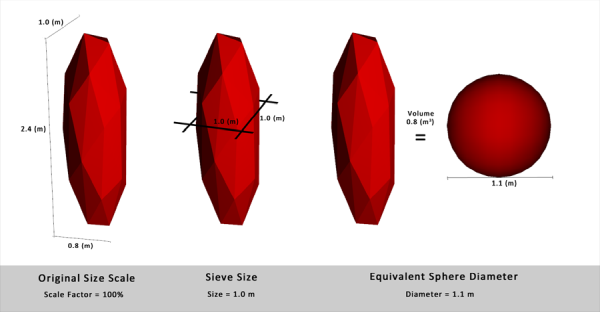
Note: The Particles Details window for the particle set will reflect the size of only the largest particle in the Particle set.
Tip: To show the exact size of your imported shape within the Particle Details window, use the Original Scale Size for Size Type and set the biggest size to 100%.
The PSD in Rocky is linear by Particle Mass or, on a semi-log scale, by the resulting particle size, and not by number. When you enter the percentage of cumulative mass and then either particle sieve Size, sphere Diameter, or original size Scale Factor (representing the three available Size Types, respectively), these represent points on a semi-log plot. Anything between two points follows the linear rule:

For rigid particles composed of Single Elements, a range of sizes, diameters, or scale factors can be defined for the PSD. For flexible or rigid particles composed of Multiple Elements (also known as meshed particles-see the Composition Tab section below), only one size, diameter, or scale factor should be defined per Particle set.
(See also Set Particle Size Ranges.)
For simulations with Coarse Grain Modeling enabled (see also About Physics Parameters), there will be an additional option on the Size tab (Figure 9).
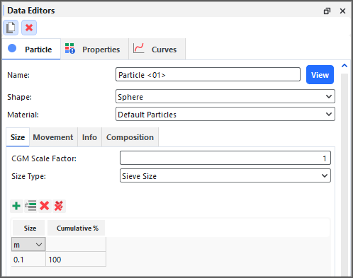
The purpose of this additional option is to increase the particle size while maintaining the system behavior using a reduced number of (larger) particles. For example, you can study the behavior of smaller particles-for example, those measured in micrometers or microns (μm)-without having the computational cost of simulating each tiny particle individually. Rather than creating an impractical case involving, perhaps, many thousands of millions of tiny particles, you can analyze the same case but with a reduced number of bigger particles.
This is accomplished by allowing you to specify a unique CGM Scale Factor for each of your Particle sets, which enables you to define a much larger, easier-to-process particle whose main purpose is to represent the behavior of a certain amount of smaller particles within your simulation.
When used, the CGM Scale Factor employs a series of corrections to the larger, representative particle in order to achieve physical behavior coherence with the size of the smaller, real-sized particle. It also ensures that the thermal model, contact model, and various forces used in the simulation will be modified to take into account the characteristics of the smaller, real-sized particle. When a Rocky simulation is carried out with CFD Coupling, the CGM scale Factor will also modify the correlations for drag and thermal properties in a similar manner.
The Orientation tab (Figure 10) is where you define what direction your particles will enter the domain.

By default, particles are injected into the domain perpendicular to the inlet (Figure 11). As shown in the examples below, you can change the default orientation in relation to the inlet to have all particles come in at a different angle (Figure 12), have particles come in at random angles (Figure 13), and many options in between.
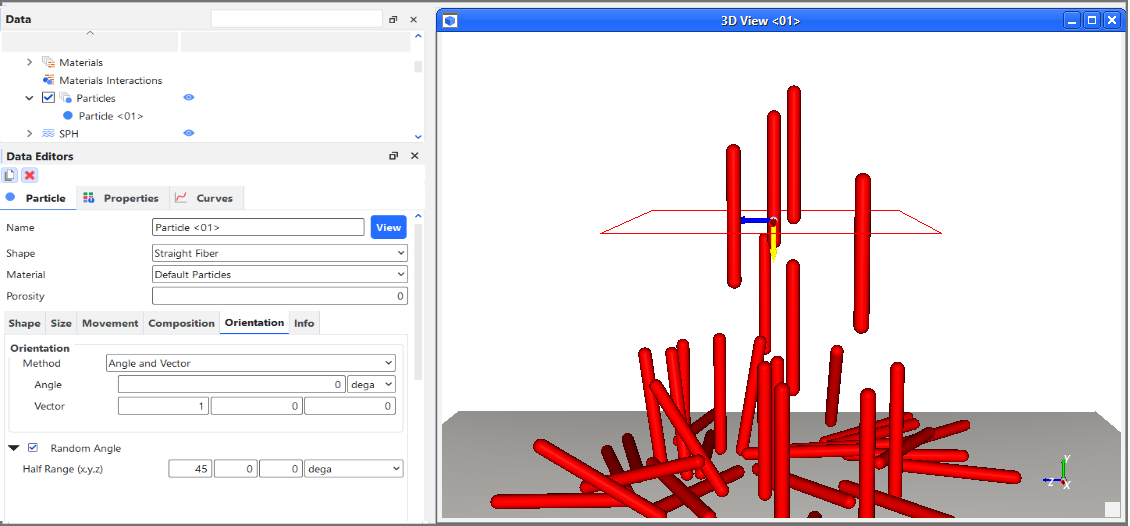
Figure 3.140: A Particle set with a 45 degree Rotation Angle along the X axis being released from an inlet
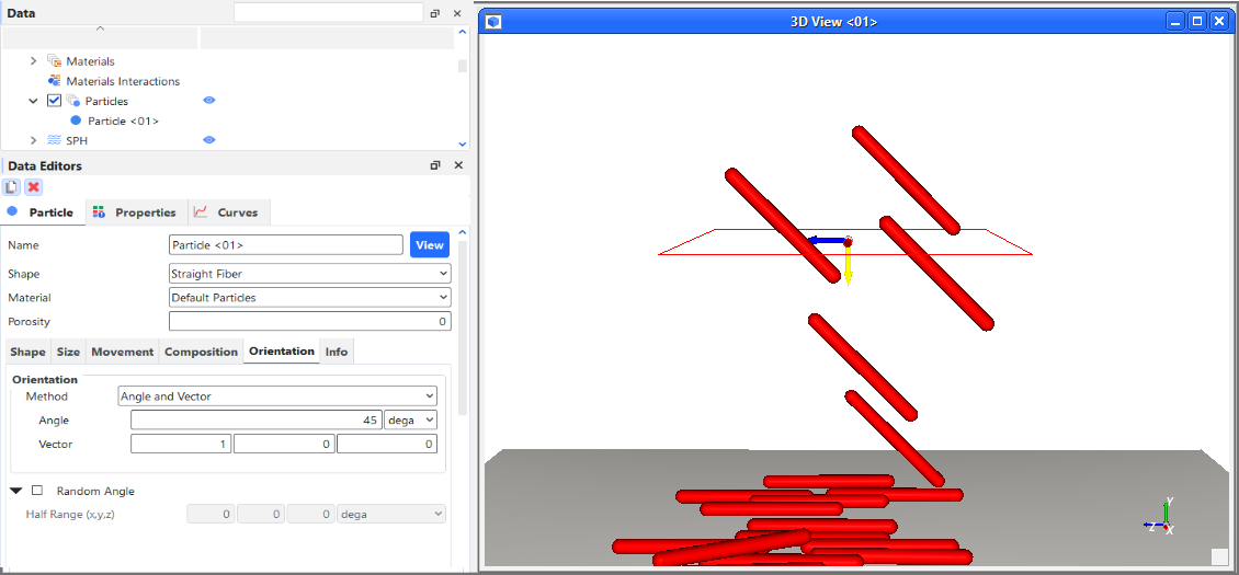
Figure 3.141: A Particle set that allows random orientations within 45 degrees of the X axis being released from an inlet
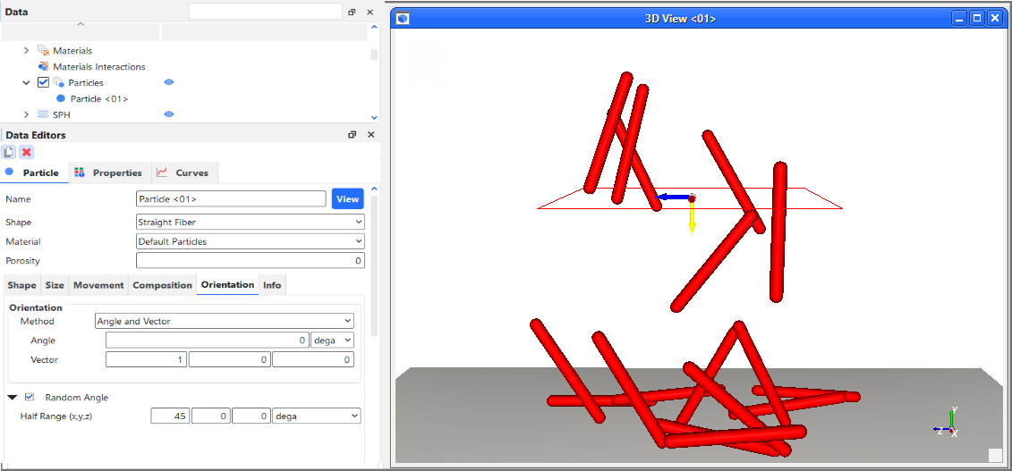
Important: The orientation of the Particle is in relation to the orientation of the inlet from which the Particle set is released. (See also About Adding and Editing Particle Inputs.)
Fixed (i.e., not random) particle orientations can be previewed in the Particles Details window (Figure 14). For particles with random orientations, the Particles Details will show only the base orientation off of which the random orientations will be calculated.
Figure 3.142: Particles Details window showing example particle rotated 90 degrees in the Z direction
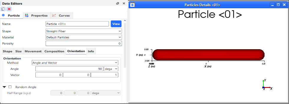
The Movement tab includes the rolling resistance, rotations, and (for non-Assembly shapes only) particle mass parameters that you can apply to a Particle set, as shown in Figure 15. For Assembly particle shapes (Figure 15a), the mass properties are calculated automatically by Rocky unless you have decided to override these values by using the Custom Properties tab. (See also the Custom Properties Sub-Tab section below.)
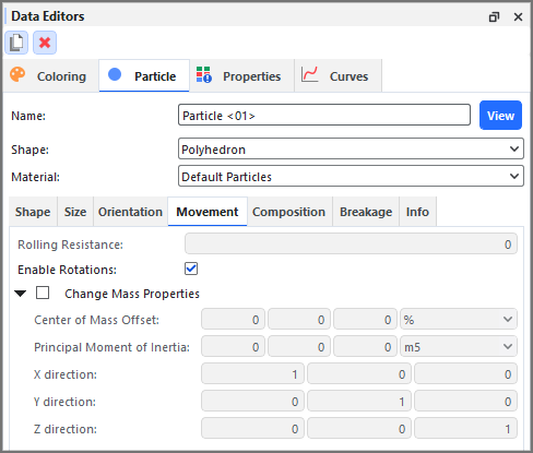
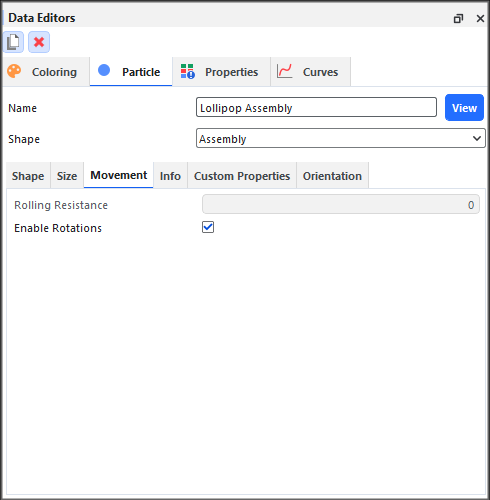 Figure 15a: Particle, Movement tab on the Data Editors panel for an Assembly particle shape
The Rolling Resistance value can be set only after a Rolling Resistance Model has been defined in the Physics | Momentum tab. (See also About Physics Parameters.) In addition, Rolling Resistance can be set only for rigid particles that are convex in shape. Therefore, flexible particles and concave-shaped rigid particles will always have zero (0) Rolling Resistance.
Enable Rotations can be edited only for rigid particles. Therefore, flexible particles will always have Enable Rotations turned on. Note: Although flexible particles will always include rotations, you can use the Include Rotational Deformations checkbox on the Breakage sub-tab if you want to disregard stresses caused by rotational deformations (bending or torsion) when considering Discrete Breakage criteria.
While any non-Assembly particle shape can make use of them, Particle mass properties are intended primarily for custom imported particle shapes (see also About Defining and Importing Custom Particle Shapes) and can be used to shift the particle's center of mass and/or override its moment of inertia.
The Custom Properties tab (Figure 15b) is for Assembly particle shapes and should be used only if the following criteria are met:
Two or more parts making up your Assembly particle overlap.
The Rocky-defined Mass, Area, Volume and other properties are not accurate enough for your simulation purposes.
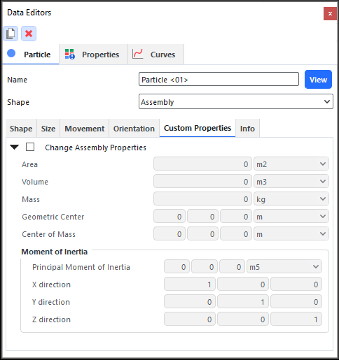
Figure 15b: Particle, Custom Properties tab on the Data Editors panel for Assembly particle shapes
If you decide to define your own Custom Properties for Assembly shape, you can discover the values you need from the CAD program with which you designed your ideal (Assembly) particle shape.
The Composition tab contains the meshing and flexibility and joint plasticity models that are available for the selected Particle set (Figures 16-17).


Figure 3.146: Particle, Composition tab for Fibers when both Anisotropic and Bilinear Elastoplastic Joint Model are enabled
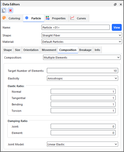
By default, each Rocky particle is generated as a single, undivided, inflexible element. When Multiple Elements are selected as the Composition however, the particle shape will be composed of many separate Elements. Rocky calculates these separate elements by applying a meshing model, which enables the particle to become flexible if desired, and in the case of Fibers, can also provide additional detail when coupled with CFD fluid forces.
Meshing is implemented in different ways depending upon which kind of shape you select, as described in Table 4 below.
Table 4: How meshing is implemented in different particle shapes
Solid Shapes (3D) (Polyhedron and Custom Polyhedron only) | Shell Shapes (2D) | Fiber Shapes (1D) |
|---|---|---|
|
|
|
When Multiple Elements are selected, Solid shapes are divided into a minimum amount of tetrahedrons that are (roughly) equal in volume. The number of tetrahedrons can be (roughly) increased by using the Target Number of Elements field, but can only be decreased to the minimum amount of elements calculated by Rocky. | By default when Multiple Elements are selected, Shell shapes are divided into a minimum amount of triangles that are (roughly) equal in area. The number of triangles can be (roughly) increased by using the Target Number of Elements field, but can only be decreased to the minimum amount of elements calculated by Rocky. When the Remesh to Target checkbox is cleared, however, Shell shapes are divided along the same triangular segments of the geometry's imported .stl file. In this situation, the number of triangle elements can only be increased or decreased in the .stl file itself (using a CAD program, such as Ansys SpaceClaim) and then re-imported into Rocky. | When Multiple Elements are selected, Fiber shapes are divided into "links" of (roughly) equal length. The number of divisions can be (roughly) increased or decreased by using the Target Number of Elements field. |
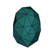
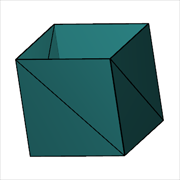

You can choose (roughly) how fine to mesh your particle by entering the Target Number of Elements you want. Because each particle shape will have different minimum element amounts, and different element ranges outside of which the meshing cannot maintain the integrity of the selected shape, Rocky helps you set an appropriate value in the following two ways:
By indicating the minimum number of elements in an error message located at both the bottom of the Data Editors panel and within the Status panel (Figure 19).
By providing how many actual Elements (or tessellations) the particle will be composed of via the Elements value on the Particle | Info sub-tab. (See also the Info Tab section below.)
Figure 3.147: Example error messages shown when a Target Number of Elements value is below the minimum calculated by Rocky
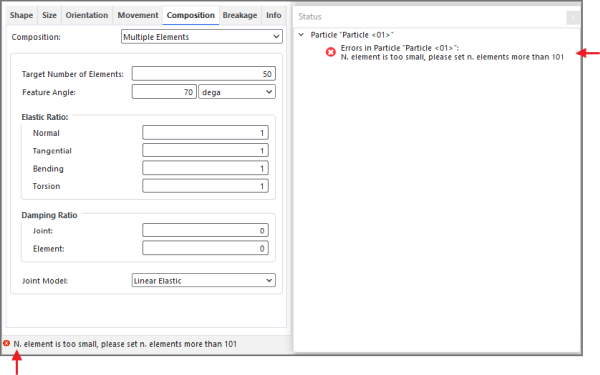
Besides (roughly) controlling the quantity of the individual Elements, for Solid and Shell particles Rocky also allows you to (roughly) control the shape of the individual Elements that make up the meshed particle. In cases where the original particle is made up of triangles with sharp edges, the meshing process can change the angles of those edges resulting in a final particle shape that can differ-perhaps undesirably-from the original. It is for this reason that Rocky provides an Feature Angle parameter (Figure 20) that enables to you specify how much of the original triangular edges are preserved during meshing, and how many are ignored. In this way, you can have more control over the final shape of your meshed particle, while still retaining its ability to become flexible.
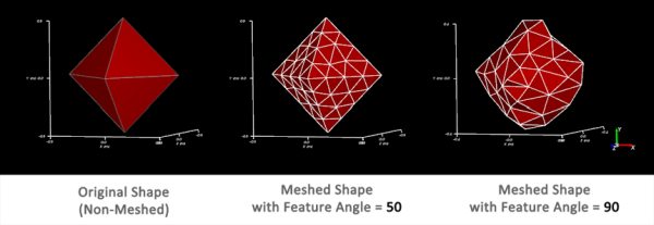
Note: The value you set for Feature Angle can influence the minimum amount of Elements required by Rocky.
Tip: You can visualize the individual Elements in the Particles Details window by turning on Edges from the Coloring tab.
The Breakage tab settings determine how the particles break and fragment upon contact with other particles or boundaries (Figure 21).
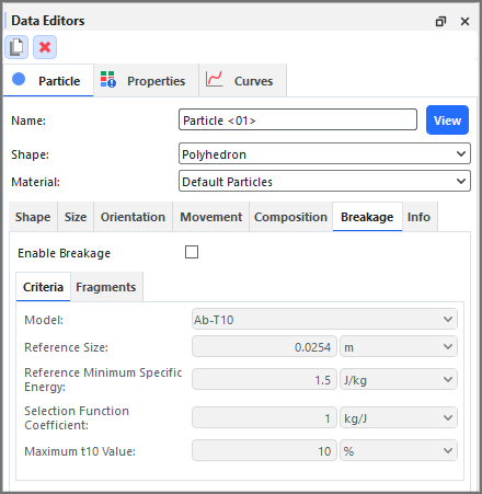
Both the Shape and the Composition of your particle set will determine whether or not breakage modeling is available, and whether Instantaneous Breakage or Discrete Breakage models can be applied. (See also About Particle Breakage.)
In this version of Rocky, only the following Shape | Composition option combinations support breakage calculations (Table 5).
Table 5: Shape Type and Composition Combinations that Support Breakage Calculations
Shape Type | Composition |
|---|---|
Either Straight or Custom Fiber | Multiple Element |
Custom Shell | Multiple Element |
Solid Polyhedron | Either Single or Multiple Element |
Solid Briquette | Single Element |
Solid Faceted Cylinder | Single Element |
Solid Custom Convex Polyhedron | Either Single or Multiple Element |
Solid Custom Concave Polyhedron | Multiple Element |
Once you choose a compatible particle shape and composition, there will be two kinds of breakage models available: one set of Instantaneous Breakage models for rigid particles composed of only a Single Element, and another set of Discrete Breakage models that are specific for flexible particles composed of Multiple Elements.
For single-element particles, the Instantaneous Breakage models available include the Ab-T10 and the Tavares models. Both models preserve both mass and volume.
Note: In this version of Rocky, the TBM breakage model is provided as an external module. Refer to the Install an External Module topic for details.
For multi-element (flexible) particles, the Discrete Breakage models available include Griffith Energy Criterion, Shear Stress Criterion, Tensile Stress Criterion, Tensile or Shear Stress Criterion, and von Mises Stress Criterion.
Depending upon which breakage Model you choose, different settings will be provided (Figures 22-28).
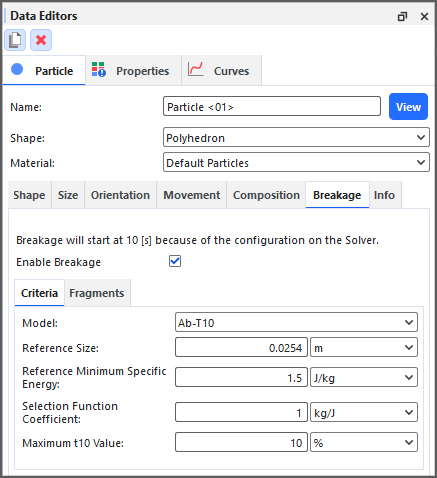
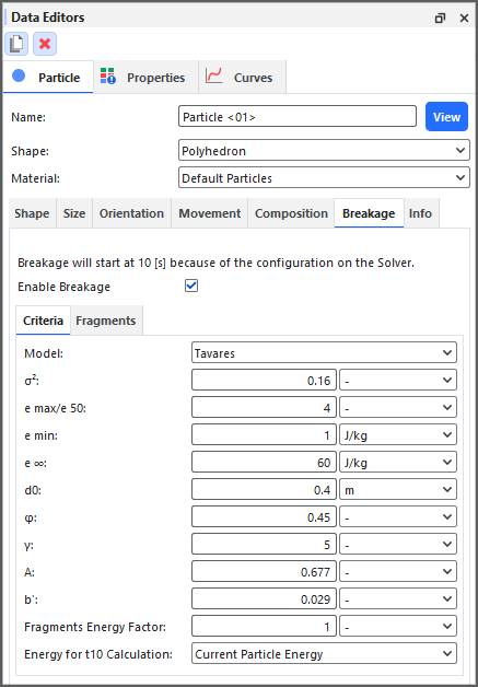
Figure 3.152: Particle, Breakage tab on the Data Editors panel showing the Griffith Energy Criterion model settings
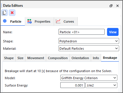
Figure 3.153: Particle, Breakage tab on the Data Editors panel showing the Shear Stress Criterion model settings
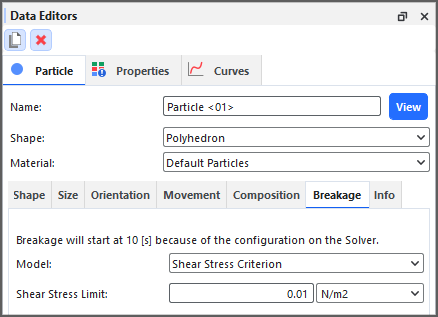
Figure 3.154: Particle, Breakage tab on the Data Editors panel showing the Tensile Stress Criterion model settings
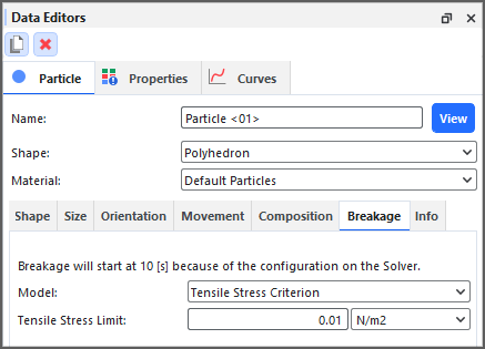
Figure 3.155: Particle, Breakage tab on the Data Editors panel showing the Tensile or Shear Stress Criterion model settings
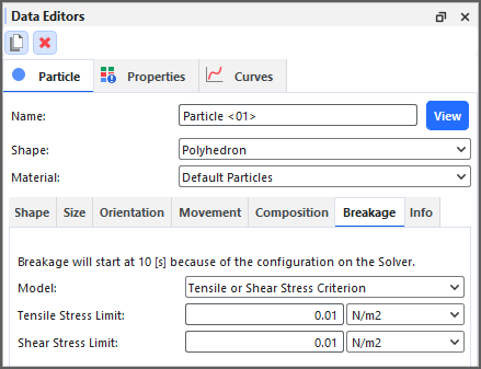
Figure 3.156: Particle, Breakage tab on the Data Editors panel showing the von Mises Stress Criterion model settings
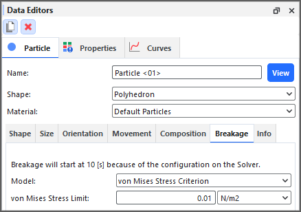
In addition, the Instantaneous Breakage models will have additional options on the Fragments sub-tab (Figures 29-30).
Note: There are no fragment distribution options provided for the Discrete Breakage models.
Figure 3.157: Particle, Breakage, Fragments sub-tab on the Data Editors panel showing the Gaudin-Schumann distribution model
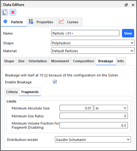
Figure 3.158: Particle, Breakage, Fragments sub-tab on the Data Editors panel showing the Incomplete Beta distribution model
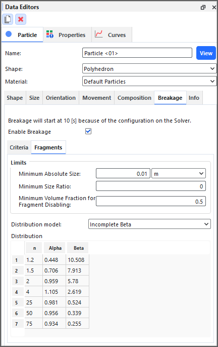
The Info tab provides more details about the parameter set that you defined, and can help you determine whether the settings you have will meet your needs (Figure 31).
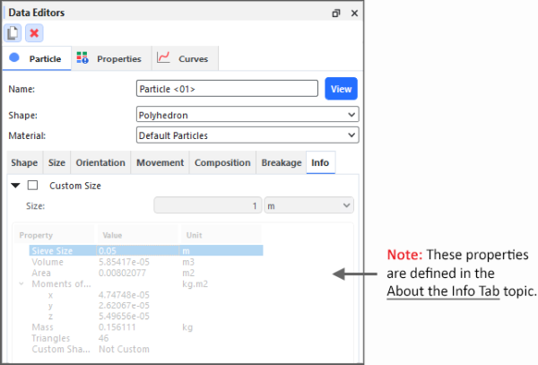
To keep you from having to switch from tab to tab, a Custom Size parameter is provided which when selected, enables you to experiment with alternate particle sizes and immediately see how it affects the property values listed, such as particle Mass and number of Elements. Once you arrive at a Custom Size you like, you can then go back to the Size tab and make your final changes accordingly.
Tips:
To learn more about the properties listed at the bottom of the Info tab, refer also to the About the Info Tab topic.
Unlike other Info tabs in Rocky, you can change what is used in the Unit column by clicking the unit you want to change and selecting a new option from the list that appears.
If you have enabled a module that affects your individual Particle set settings, you might also have a separate Modules sub-tab with additional settings that you can define (Figure 32). Refer to the Module's documentation (if provided) for more information. (See also Rocky Simulation Entities that can be Affected by Modules.)

See the tables below (and refer to the images above) to help you understand how to add and edit particle sets.
Table 6 : Main Particle tab options (Figure 1 above)
Setting | Description | Range |
|---|---|---|
Name | Enables you to specify a unique identifier for the particular Particle set. | 99 character limit |
Shape | The initial default (and custom imported) shapes you can use as starting point for defining your final particle shape. Most default shapes have Shape attributes that you can use to modify the shape further. (See also About Defining and Importing Custom Particle Shapes). | Solid shapes:
Fiber shapes:
Shell shapes:
Assembly shapes:
|
Material | Defines the density and Young's Modulus of the Particle set based upon the options you've defined in the Materials list. (See About Modifying Material Compositions for more information.) | List is based upon the Materials that have been defined |
| Porosity | Defines the particle porosity percentage, according to the particle type. | Positive values |
Table 7 : Particle, Shape sub-tab options (Figures 2-6 above)
Setting | Description | Range |
|---|---|---|
Solid and Fiber Shape Settings | ||
Vertical Aspect Ratio | Changes the height (Y value) of the particle assuming a Z value of 1. | Value limited by list box. Note: The upper limit for the shapes that allow this setting are provided below:
|
Horizontal Aspect Ratio | Changes the width (X value) of the particle assuming a Z value of 1. | Value limited by list box |
Smoothness | Changes how smooth or sharp the particle edges are. The higher the value, the smoother the edges. | Value limited by list box |
Side Angle | For Briquettes, changes the angle of the corners. | Value limited by list box |
Number of Corners | Changes how many points a particle's surface has. | Value limited by list box |
Superquadric Degree | Changes how square or elliptical a particle appears. The higher the value, the more square the shape. | Value limited by list box |
Shell Shape Settings | ||
Thickness | For Shell particles, this determines the current absolute thickness of each 2D plane that makes up the shape, using as its baseline the original size of the imported shape at 100% scale. The value entered is reflected in the Particles Details window and affects the resulting mass of the particle as well as the number of Element that are required to make it flexible (also known as Meshed). Important: This value is based only on the original, imported size of the particle and does not take into account changes to the size of your particle. However, a corresponding thickness will be applied to all particles in your set, regardless of their size. Tip: For best results, adjust the Thickness only when viewing the particle at 100% Original Size Scale. (See Table 6 below.) | Positive values |
Assembly Shape Settings | ||
Particle | For Assembly shapes only, this is the Particle set whose shape you want to use as a part within your final Assembly. Note: For Particle Assembly the porosity parameter will be defined for each particle that makes up the assembly. Moreover, it is possible to define the porosity in the field Custom Properties. | Any Particle set defined as single element (rigid), non-breakable or Straight shape. |
PX | For Assembly shapes only, this is the part's position on the X axis. Note: The Particles Details window shows only the part's position relative to the gravity center of the whole Assembly. | Any value |
PY | For Assembly shapes only, this is the part's position on the Y axis. Note: The Particles Details window shows only the part's position relative to the gravity center of the whole Assembly. | Any value |
PZ | For Assembly shapes only, this is the part's position on the Z axis. Note: The Particles Details window shows only the part's position relative to the gravity center of the whole Assembly. | Any value |
Scale | For Assembly shapes only, this determines the part's size relative to the largest size of the PSD that is defined on the Size tab for the original Particle set. For example:
| Any value |
RX | For Assembly shapes only, this is the X component that defines the vector about which the part is rotated. This is used in conjunction with the Angle parameter to define the final orientation of the part. | No limit but the values entered will be normalized |
RY | For Assembly shapes only, this is the Y component that defines the vector about which the part is rotated. This is used in conjunction with the Angle parameter to define the final orientation of the part. | No limit but the values entered will be normalized |
RZ | For Assembly shapes only, this is the Z component that defines the vector about which the part is rotated. This is used in conjunction with the Angle parameter to define the final orientation of the part. | No limit but the values entered will be normalized |
Angle | For Assembly shapes only, this is the degree of rotation about the defined rotation vector (RX, RY, and RZ). | No limit |
Table 8: Particle, Size sub-tab options (Figures 7-9 above)
Setting | Description | Range |
|---|---|---|
CGM Scale Factor | When Coarse Grain Modeling is enabled (see also About Physics Parameters), this scale factor will be applied to the particle Size (Diameter or Scale Factor) you enter to determine the final simulated size of the particle and how many smaller particles' behavior it represents. Specifically:
Note: If more one Size row is specified for the Particle set, the same scale factor will be applied to all particle sizes in the set. (See also I cannot find Particle Size Scale Factor). | 1.0 or greater |
Size Type | Determines how the size of the particle will be measured. Specifically:
| Sieve Size; Equivalent Sphere Diameter Original Size Scale |
Size | When Sieve Size is set for Size Type, this is the dimension of the mesh sieve that determines particle size. Note: For particles composed of only a Single Element (see also Composition Tab section above), more than one size row can be specified if desired. For particles composed of Multiple Elements, only one size may be specified. If only one size is specified for a particle set, only particles of that size will be used during the simulation. This is because the smallest Size value specified will always have no range. If more than one size is specified for a particle set, a range of sizes within the Size parameter will be used for each Cumulative % provided. The one exception is for the smallest Size value, which will have no range. For example, for the sizes and percentages specified below:
See also Set Particle Size Ranges. | Positive values; sizes should decrease as you go down the Size table |
Diameter | When Equivalent Sphere Diameter is set for Size Type, this is the diameter of a sphere that has a volume equivalent to that of the particle, which determines particle size. Note: For particles composed of only a Single Element (see also Composition Tab section above), more than one diameter row can be specified if desired. For particles composed of Multiple Elements, only one diameter row may be specified. If only one diameter is specified for a particle set, only particles of that equivalent diameter will be used during the simulation. This is because the smallest Diameter value specified will always have no range. If more than one diameter is specified for a particle set, a range of diameters within the Diameter parameter will be used for each Cumulative % provided. The one exception is for the smallest Diameter value, which will have no range. For example, for the diameters and percentages specified below:
See also Set Particle Size Ranges. | Positive values; diameters should decrease as you go down the Diameter table |
Scale Factor | When Original Size Scale is set for Size Type, this is the percentage or factor of the original particle size to which the new particle size should be scaled. Note: For particles composed of only a Single Element (see also Composition Tab section above), more than one scale factor row can be specified if desired. For particles composed of Multiple Elements, only one scale factor row may be specified. If only one scale factor is specified for a particle set, only particles of that resulting size will be used during the simulation. This is because the smallest Scale Factor value specified will always have no range. If more than one scale factor is specified for a particle set, a range of resulting sizes within the Scale Factor values will be used for each Cumulative % provided. The one exception is for the smallest Scale Factor value, which will have no range. For example, for the diameters and percentages specified below:
See also Set Particle Size Ranges. | Positive values; factors should decrease as you go down the Scale Factor table |
Cumulative % | When more than one size, diameter, or scale factor are specified for a particle set, this is the percentage of particle mass that will be devoted to that particular sieve size, sphere diameter, or original scale factor range. The first row (top most value) should represent the largest particle size in the set. Subsequent rows should represent decreasingly smaller sizes as needed. (See also Size, Diameter, or Scale Factor descriptions above.) See also Set Particle Size Ranges. | 0<100; values should decrease as you go down the respective Size, Diameter, or Scale Factor tables |
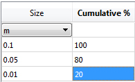
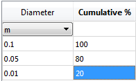
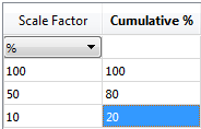
Table 9: Particle, Orientation sub-tab options
Setting | Description | Range |
|---|---|---|
Orientation | ||
Method |
Enables you to select how you want to define the orientation of the particle shape. Specifically:
| Angles; Angle and Vector; Basis Vectors. |
Method Angles | ||
Order | When Angles is selected for Orientation, this defines the order in which the three Rotation text fields will be applied. | XYZ; ZXY; YXZ; YZX; ZXY; ZYX. |
Local Angles |
When Angles is selected for Orientation, this defines what coordinate system will be used as a basis for the angle specified. Specifically:
| Turns on or off |
| Rotation | When Angles is selected for Orientation, this is the degree of particle rotation in each of the three directions specified by the Order provided. | Any value |
| MethodAngle and Vector | ||
| Angle | When Angle and Vector is selected for Orientation, this is the angle the cube will rotate around the Vector defined. | Any value |
| Vector | When Angle and Vector is selected for Orientation, this is the X, Y, and Z components that define the vector around which the particles will rotate, using the Angle defined. | No limit but the values entered will be normalized |
| MethodBasis Vectors | ||
| X direction |
When Basis Vectors is selected for Orientation, this is the coordinate values defining the first of three directional vectors that together define the final orientation of the particle.
Tip: To ensure correct results, make sure you define this vector as orthogonal (perpendicular) to the other two vectors.
| No limit but the values entered will be normalized |
| Y direction | When Basis Vectors is selected for
Orientation, this is the coordinate values
defining the second of three directional vectors that together define the final
orientation of the particle. Tip: To ensure correct results, make sure you define this vector as orthogonal (perpendicular) to the other two vectors. | No limit but the values entered will be normalized |
| Z direction | When Basis Vectors is selected for
Orientation, this is the coordinate values
defining the third of three directional vectors that together define the final
orientation of the particle. Tip: To ensure correct results, make sure you define this vector as orthogonal (perpendicular) to the other two vectors. | No limit but the values entered will be normalized |
| Random Angle | ||
| Half Range (x, y, z) |
Defines the X, Y, and Z angle limits within which Rocky will randomly orient each individual particle within the Particle set. Tips:
| No limit |
Table 10: Particle, Movement sub-tab options (Figure 15-15a above)
Setting | Description | Range |
|---|---|---|
Rolling Resistance | When a Rolling Resistance Model is defined on the Physics | Momentum tab (see also About Physics Parameters), this setting changes how particle shapes that are both rigid and convex roll on the boundary surface. A higher value reduces rolling. Tips:
Note: Neither Flexible particles nor concave-shaped rigid particles support editing this value; as a result, it will always be set to zero (0) for these shapes. See Also: | 0 - 1 |
Enable Rotations | When selected for rigid particle shapes, allows the particle to rotate during the simulation. Note: Flexible particles do not support editing this value; as a result, it will always be selected (enabled) for these shapes. | Turns on or off |
Change Mass Properties | When enabled (for non-Assembly shapes only), this allows you to change the position of the particle's center of mass and moment of inertia values. Tips:
| Turns on or off |
Center of Mass Offset | When Change Mass Properties is enabled, these three values specify the displacement of the particle's center of mass relative to its geometric center in the X, Y, and Z directions, expressed as percentages of the particle's sieve size. This relationship can be described as:
For example, if a
particle of Sieve
Size | -50% to +50% |
Principal Moment of Inertia | When Change Mass
Properties is enabled,
these are the particle's
principal
moments of inertia
along the X, Y, and Z
axes defined below. The
values you enter
should be defined
based upon the
Center of Mass
Offset position you
have set, and
should assume the
particle has a sieve
size equal to
Note: The units here indicate that the values you provide should be the moment of inertia divided by the density. This is different than the Moment of Inertia Property calculated during post-processing. (See also About Properties). | Positive values greater than but not equal to zero |
X direction | The X, Y, and Z components that define the X axis for the Principal Moment of Inertia. Note: This is based upon the global coordinate system. | No limit but the values entered will be normalized, and the base must be positive orthonormal |
Y direction | The X, Y, and Z components that define the Y axis for the Principal Moment of Inertia. Note: This is based upon the global coordinate system. | No limit but the values entered will be normalized, and the base must be positive orthonormal |
Z direction | The X, Y, and Z components that define the Z axis for the Principal Moment of Inertia. Note: This is based upon the global coordinate system. | No limit but the values entered will be normalized, and the base must be positive orthonormal |


Table 10a: Particle, Custom Properties sub-tab options (Figure 15b above)
Setting | Description | Range |
|---|---|---|
Change Assembly Properties | When enabled for Assembly particle shapes, this allows you to enter the values of Area, Volume, Geometric Center, Center of Mass and other properties from the CAD program with which you designed your Assembly particle shape. | Turns on or off |
Area | The Area of your Assembly particle. | Positive values greater than but not equal to zero. |
Volume | The Volume of your Assembly particle. | Positive values greater than but not equal to zero. |
Geometric Center | The Geometric Center you want to set for your particle assembly. | Coordinates inside the particle bounding box. |
Center of Mass | The Center of Mass you want to set for your particle assembly. | Coordinates inside the particle bounding box. |
Moment of Inertia | When Change Assembly
Properties is enabled,
these are the particle's
principal
moments of inertia
along the X, Y, and Z
axes defined below. The
values you enter
should be defined
based upon the
Center of Mass
position you
have set, and should
assume the particle has
an Original Size Scale
equal to Note: The units here indicate that the values you provide should be the moment of inertia divided by the density. This is different than the Moment of Inertia Property calculated during post-processing. (See also About Properties). | Positive values greater than but not equal to zero |
X direction | The X, Y, and Z components that define the X axis for the Principal Moment of Inertia. Note: This is based upon the global coordinate system. | No limit but the values entered will be normalized, and the base must be positive orthonormal |
Y direction | The X, Y, and Z components that define the Y axis for the Principal Moment of Inertia. Note: This is based upon the global coordinate system. | No limit but the values entered will be normalized, and the base must be positive orthonormal |
Z direction | The X, Y, and Z components that define the Z axis for the Principal Moment of Inertia. Note: This is based upon the global coordinate system. | No limit but the values entered will be normalized, and the base must be positive orthonormal |
Table 11: Particle, Composition sub-tab options (Figure 16-20 above)
Setting | Description | Range |
|---|---|---|
Composition | Determines whether the particle will be composed of one or many Element. Specifically:
Note: Only Fibers, Shells, and Polyhedron and Custom Polyhedron (Solid) shapes are currently able to be meshed. (See also Program Limitations). | Single Element; Multiple Elements |
Remesh to Target | For Shell particles only, defines how the triangular elements that make up the shape surface are determined. Specifically:
| Turns on or off |
Target Number of Elements | When Multiple Elements are selected, this allows you to (roughly) control the number of individual Element that will comprise your particle shape. The higher the value, the more accurate the representation but the longer the processing time due to the increased calculations. Tips:
| Positive values |
Feature Angle | For Solid and
and Shell particles,
when Multiple
Elements
are selected, this
sets the angle limit at
which the meshing
algorithm in Rocky will
try to preserve the
edges of the
triangular components
that make up the base
shape when turning them
into individual
Element. An edge is
defined as the line that
connects two
triangles and the
feature angle is the
angle between the two
triangles' normals
(Figure 21).
Changing this setting is useful for particle shapes containing triangles with sharp edges where the default meshing calculations generate individual Element shapes that change the sharp parts of the original particle shape. in an undesirable way (Figure 14). Tip: You can visualize the shape of the individual Elements in the Particles Details window by turning on Edges from the Coloring tab. | 0-180 |
Elasticity | When Multiple Elements are selected, this determines how the elasticity of the joint between the individual Element are treated. Specifically:
| Isotropic; Anisotropic |
Elastic Ratio | When Multiple Elements are selected, and Isotropic is selected for Elasticity, this determines the degree of flexibility of the particle. Formally, this parameter is defined as the ratio of the Young's modulus of the joints to the bulk Young's modulus defined for the particle's material. (See also About Modifying Material Compositions). | There are two sets of ranges:
Tip: To avoid either too soft or too rigid particles, it is recommended that you use values closer to 1.0 |
Elastic Ratio Normal | When Anisotropic is selected for Elasticity, this defines the degree of flexibility in the Normal direction. | 1e-5 - 1 (non-Fiber shapes only) 1e-5 - 100 (Fiber shapes only) |
Elastic Ratio Tangential | When Anisotropic is selected for Elasticity, this defines the degree of flexibility in the Tangential direction. | 1e-5 - 1 (non-Fiber shapes only) 1e-5 - 100 (Fiber shapes only) |
Elastic Ratio Bending | When Anisotropic is selected for Elasticity, this defines the degree of flexibility when the particle is bent. | 1e-5 - 1 (non-Fiber shapes only) 1e-5 - 100 (Fiber shapes only) |
Elastic Ratio Torsion | When Anisotropic is selected for Elasticity, this defines the degree of flexibility when the particle is twisted. | 1e-5 - 1 (non-Fiber shapes only) 1e-5 - 100 (Fiber shapes only) |
Damping Ratio Joint | When Multiple Elements are selected, this determines the degree of decay of oscillations of the joint between the individual Elements that compose the particle, and is applied as joint forces and moments proportional to the respective joint deformation velocities. It is effective in reducing or removing high-frequency oscillations. | 0-1 |
Damping Ratio Element | When Multiple Elements are selected, this determines the degree of decay of oscillations among the Elements that compose the particle, and is applied as Element forces proportional to difference between the Element velocity and the velocity of the center of mass of the particle to which the Element belongs. It is effective in reducing or removing oscillations of low frequency. | 0-1 |
Conductivity Ratio | When both the Thermal Model is enabled (see also About Physics Parameters) and Multiple Elements are selected, this enables you to increase or reduce the heat transfer between Element relative to the heat transfer associated to collisions with other particles or boundaries. | 0.01 - 100 |
Joint Model | When Multiple Elements are selected, this defines the plasticity model being used to simulate the movements between the joint of the individual Element. Specifically:
| Linear Elastic; Bilinear Elastoplastic Note: If you have an external Module that adds in an additional Joint Model, you must use that model at least once in your simulation project if the Module is enabled. Refer to the Module's documentation (if provided) for more information. (See also Rocky Simulation Entities that can be Affected by Modules). |
Plastic Ratio | When Multiple Elements is selected and also Bilinear Elastoplastic is selected for Joint Model, this defines the ratio between the stiffness in the elastoplastic regime to the stiffness in the elastic regime. The smaller the value of this ratio, the more evident will be the permanent deformations on the joints. | 0-1 |
Torsion Angle Limit | For Shell and Fiber particle shapes only, when Multiple Elements is selected and also Bilinear Elastoplastic is selected for Joint Model, this defines the limit of the purely elastic regime on the bilinear elastoplastic model, for torsion deformation. | 0-360 degrees |
Bending Angle Limit | For straight and custom Fiber particle shapes only, when Multiple Elements is selected and also Bilinear Elastoplastic is selected for Joint Model, this defines the limit of the purely elastic regime on the bilinear elastoplastic model, for bending deformations. | Positive values |
1st Bending Angle Limit | For custom Shell particle shapes only, when Multiple Elements is selected and also Bilinear Elastoplastic is selected for Joint Model, this defines the limit of the purely elastic regime on the bilinear elastoplastic model, for bending deformations in the direction perpendicular to the thickness of the shell Element. | 0-180 degrees |
2nd Bending Angle Limit | For custom Shell particle shapes only, when Multiple Elements is selected and also Bilinear Elastoplastic is selected for Joint Model, this defines the limit of the purely elastic regime on the bilinear elastoplastic model, for bending deformations in the direction parallel to the thickness of the shell Element. | 0-180 degrees |
With Failure | For custom Fiber and Shell particle shapes only, when Multiple Elements is selected and also Bilinear Elastoplastic is selected for Joint Model, this allows you to add a sudden drop on the joint resistance to deformations when the angular deformation reaches the limiting value that controls the elastoplastic regime transition. | Turns on or off |
Failure Ratio | For custom Fiber and Shell particle shapes only, when Multiple Elements is selected and also Bilinear Elastoplastic is selected for Joint Model, this allows you to control the amount of drop on the joint resistance when the angular deformation reaches the limiting value that controls the elastoplastic regime transition. | 0-1 |
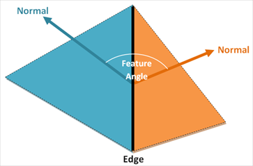
Table 12: Particle, Breakage sub-tab options for Single Element Particles (Figures 21-23 and 29-31 above)
Setting | Description | Range |
|---|---|---|
Enable Breakage | For Particle sets composed of Single Elements, this determines whether Instantaneous Breakage calculations will be taken into account during the simulation. | Turns on or off |
Criteria tab | tab | tab |
Model | Defines which method of Instantaneous Breakage calculations will be enabled during the simulation.
Important: Both Shape and Composition determine whether a particle set supports breakage and the models available. (See also About Particle Breakage). Tip: Refer to DEM Technical Manual for further detail on the specific models. (From the Rocky Help menu, point to Manuals, and then click DEM Technical Manual.) | Ab-T10; Tavares Note: If you have an external Module that adds in an additional Breakage Model, you must use that model at least once in your simulation project if the Module is enabled. Refer to the Module's documentation (if provided) for more information. (See also Rocky Simulation Entities that can be Affected by Modules). |
Ab-T10 Model Reference Size | This is the reference size used in drop weight tests. Typically, this size is 25 to 40 mm. This value and the Reference Minimum Specific Energy (for reference size) value are together used to compute the minimum specific energy for the particle. | Any positive value |
Ab-T10 Model Reference Minimum Specific Energy | This is the minimum specific energy for the Reference Size value. Both values are used to calculate the minimum specific energy for the particle. If the total specific energy for a particle that comes into contact with another particle or geometry is less than this value, breakage will not occur. This value is especially important in cases where particles break primarily on multiple impacts, such as in SAG or AG mills. For an instantaneous impact breakage event, such as with impact crushers or HPGRs, this value is not important and can set to zero. | Any positive value (zero is recommended) |
Ab-T10 Model Selection Function Coefficient | The particle breakage strength parameter, which is a material constant. Reducing this value decreases the rate of breakage. Note: This is "S" in the model equation referenced in the Potapov paper but is typically seen as "b" in other Ab-T10 equations. | Any positive value |
Ab-T10 Model Maximum t10 Value | Maximum degree of breakage. Though this value does not affect how easily a particle will break, it does affect the size of the resulting particles after breakage. The higher the value, the finer the fragments will be after breakage. Note: This is "M" in the model equation referenced in the Potapov paper but is typically seen as "A" in other Ab-T10 equations. | 0-100 |
Tavares Model
| Refers to the | Positive values |
Tavares Model
| Refers to the Ratio | Positive values |
Tavares Model | Refers to the minimum specific energy for breakage value used in the Tavares breakage equation. (See the Rocky DEM Technical Manual for further details.) | Positive values |
Tavares Model
| Refers to the | Positive values |
Tavares Model
| Refers to the | Positive values |
Tavares Model
| Refers to the | Positive values |
Tavares Model
| Refers to the | Positive values |
Tavares Model
| Refers to the | Positive values |
Tavares Model
| Refers to the | Positive values |
Tavares Model Fragments Energy Factor | Multiplies the value of the instantaneous specific impact energy by this factor. (See the Rocky DEM Technical Manual for further details.) | Any value (Recommended range is between 0-1.) |
Tavares Model Energy for t10 Calculation | Defines how the specific fracture energy will be determined when calculating the value of the t10 parameter. (See the Rocky DEM Technical Manual for further details.) | Current Particle Energy; Median Specific Fracture Energy (e50b) |
Fragments tab | ||
Limits Minimum Absolute Size | Smallest size the particle fragments can be after breakage is applied. | Positive values |
Limits Minimum Size Ratio | Smallest size the particle fragments can be at each breakage incident, relative to the parent particle (either a whole particle or a fragment). | 0-1 Note: Values are dimensionless |
Limits Minimum Volume Fraction for Fragment Disabling | Defines the minimum volume fraction that a broken particle (fragment) can have before being considered too small to be included in calculations. (See the Rocky DEM Technical Manual for further details.) | 0-1 |
Distribution model | Type of fragment distribution size used in the model. Specifically:
(See the Rocky DEM Technical Manual for further details.) | Gaudin-Schumann; Incomplete Beta Note: If you have an external Module that adds in an additional Distribution Model, you must use that model at least once in your simulation project if the Module is enabled. Refer to the Module's documentation (if provided) for more information. (See also Rocky Simulation Entities that can be Affected by Modules). |
Distribution | When Incomplete Beta is selected for Distribution model, this displays in table rows separate n,
Alpha, and Beta value sets, which Rocky then uses with the
(See the Rocky DEM Technical Manual for further details.) Tip: While the table is limited by the seven rows provided, you can edit the values by clicking the value you want to change, and then typing the new value you want. | Positive values Note: Values are dimensionless |


Table 13: Particle, Breakage sub-tab options for Multi-Element Particles (Figures 24-28 above)
Setting | Description | Range |
|---|---|---|
Model | Defines whether Discrete Breakage calculations will be enabled during the simulation and if so, which method will be used.
Important: Both Shape and Composition determine whether a particle set supports breakage and the models available. (See also About Particle Breakage). Tip: Refer to DEM Technical Manual for further detail on the specific models. (From the Rocky Help menu, point to Manuals, and then click DEM Technical Manual.) | None; Griffith Energy Criterion; Shear Stess Criterion; Tensile Stress Criterion; Tensile or Shear Stress Criterion; von Mises Stress Criterion. Note: If you have an external Module that adds in an additional Breakage Model, you must use that model at least once in your simulation project if the Module is enabled. Refer to the Module's documentation (if provided) for more information. (See also Rocky Simulation Entities that can be Affected by Modules). |
Griffith Energy Criterion Model Surface Energy | Amount of surface energy used by the Griffith breakage model to calculate the energy balance upon which the model is based. The larger the value of the surface energy, the more resistant to breakage the joint will be. | Positive values |
Shear Stress Criterion Model Shear Stress Limit | Value that defines when a joint breaks in the Shear Stress breakage model. Whenever the shear stress experienced by a joint is larger than this limit, the joint will break. | Positive values |
Tensile Stress Criterion Model Tensile Stress Limit | Value that defines when a joint breaks in the Tensile Stress breakage model. Whenever the tensile stress experienced by a joint is larger than this limit, the joint will break. | Positive values |
Tensile or Shear Stress Criterion Model Tensile Stress Limit | Value that defines the upper limit for tensile stress that can be experienced by a joint before breaking. In this model, the joint will break whenever either this or the shear stress limit is exceeded; whichever limit is reached first will determine breakage. | Positive values |
Tensile or Shear Stress Criterion Model Shear Stress Limit | Value that defines the upper limit for shear stress that can be experienced by a joint before breaking. In this model, the joint will break whenever either this or the tensile stress limit is exceeded; whichever limit is reached first will determine breakage. | Positive values |
von Mises Stress Criterion Model von Mises Stress Limit | Value that defines the upper limit for von Mises stress - which is a combination of the tensile and shear stresses - that can be experienced by a joint before breaking. | Positive values |
Include Rotational Deformations | Available only for Fiber and Shell particle sets composed of Multiple Elements (see also the Composition Tab section above), this determines whether the stresses caused by rotational deformations (bending or torsion) are included when considering Discrete Breakage criteria. | Turns on or off |
Table 14: Particle, Info sub-tab options (Figure 32 above)
Setting | Description | Range |
|---|---|---|
Custom Size | When Sieve Size is selected for Size Type on the Size sub-tab, this allows you to experiment with how different particle sizes affect certain Particle properties-such as volume, mass, and number of Element (see also About Properties)- without switching back and forth to different Particle tabs. When enabled, Property Values (bottom of Info tab) are calculated according to the Size value entered. When cleared, Property Values reflect the information entered on the Size sub-tab. | Turns on or off |
Size | When Custom Size is enabled, the value you enter here re-calculates the Property Values listed at the bottom of the Info tab. Tip: When you arrive at a size that meets your needs, ensure you change the real size value on the Size sub-tab. Only the Size tab value, and not this experimental value, is used during the simulation. Note: This text field does not support parametric variables. (See also I cannot enter an input variable or mathematical function into a text field). | No limit |
Custom Diameter | When Equivalent Sphere Diameter is selected for Size Type on the Size sub-tab, this allows you to experiment with how different particle diameters affect certain Particle properties-such as volume, mass, and number of Element (see also About Properties)- without switching back and forth to different Particle tabs. When enabled, Property Values (bottom of Info tab) are calculated according to the Diameter value entered. When cleared, Property Values reflect the information entered on the Size sub-tab. | Turns on or off |
Diameter | When Custom Diameter is enabled, the value you enter here re-calculates the Property Values listed at the bottom of the Info tab. Tip: When you arrive at a diameter that meets your needs, ensure you change the real diameter value on the Size sub-tab. Only the Size tab value, and not this experimental value, is used during the simulation. | No limit |
Custom Scale Factor | When Original Scale Size is selected for Size Type on the Size sub-tab, this allows you to experiment with how different particle scale factors affect certain Particle properties-such as volume, mass, and number of Element (see also About Properties)- without switching back and forth to different Particle tabs. When enabled, Property Values (bottom of Info tab) are calculated according to the Scale Factor value entered. When cleared, Property Values reflect the information entered on the Size sub-tab. | Turns on or off |
Scale Factor | When Custom Scale Factor is enabled, the value you enter here re-calculates the Property Values listed at the bottom of the Info tab. Tip: When you arrive at a scale factor that meets your needs, ensure you change the real scale factor value on the Size sub-tab. Only the Size tab value, and not this experimental value, is used during the simulation. | No limit |
Table 15: Particle, Module sub-tab options (Figure 33 above)
Setting | Description | Range |
|---|---|---|
Modules | ||
(Varies) | These settings are specific to only certain external Module and are therefore not documented in the Rocky User Manual. Refer to the Module's documentation (if provided) for more information. (See also Rocky Simulation Entities that can be Affected by Modules). | (Varies) |
What would you like to do?
See Also:
An Assembly is a type of Particle set made by combining the shapes of other Particle sets to form a single, unique particle. It can be useful in cases where you are trying to replicate the glued-sphere approach common in other DEM programs (see also Clustered x polyhedral shape: why is it important to consider particle shape), but its use also leads to faster simulations when compared to using a similar custom (imported) .stl shape. (See also About Defining and Importing Custom Particle Shapes.)
Especially when using multiple convex shapes to represent a traditional concave shape (Figure 1), the computational savings of using an Assembly particle can be significant.
Figure 3.161: Traditional (imported) concave bolt shape (left) compared with the same shape defined as an Assembly particle (right)
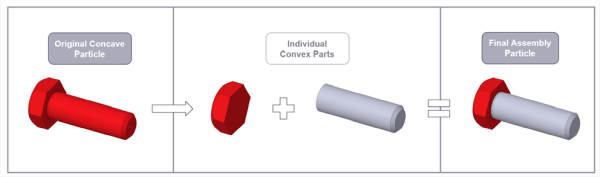
In Rocky, the shapes you combine together to form the Assembly shape are called parts. Parts are based upon Particle sets that you define separately from the Assembly itself. Once included in an Assembly, the Size, Shape, Material, and Center of Mass criteria of the original Particle set making up the part are used; all other settings (Orientation, Movement, Color, etc.) are ignored by the Assembly. This means that you can define your Assembly to be heterogeneous—by specifying different materials for each part—or homogenous by specifying same material for each part.
Once the parts are defined, the whole Assembly shape will take on its own PSD, Orientation, Movement, color, and other settings, and will behave in the simulation just like any other individual Particle set, including being able to be used in Thermal, Coarse-Graining, and CFD Coupled simulations. (For a full list of capabilities, refer to the Rocky Particle Shapes and Capabilities topic.)
In this version of Rocky, you are able to override the settings Rocky calculates for the Assembly's mass, area, volume, and other properties. This is usually necessary only if two or more parts in your Assembly particle overlap, and you require exact properties for your simulation to be successful.
To specify Custom Properties for your assembly shape, please do the following:
From the CAD program with which you designed your ideal (Assembly) particle shape, note the Area, Volume, Mass, Geometric Center, Center of Mass, and other properties you want Rocky to use for your Assembly particle shape.
In Rocky, from your Assembly particle's Particle | Custom Properties tab, enable the Change Assembly Properties checkbox, and then enter the information you want Rocky to use.
Tip: You can use the colored dots in the Particles Details window to preview where your Center of Mass (blue dot) and Geometric Center (yellow dot) are located.
In this version of Rocky, the Geometric Center for an Assembly particle is represented in the Particles Details window as a yellow dot, and the Center of Mass is represented by a blue dot. The Geometric Center and Center of Mass coincide when the density is uniform throughout the part. By default, Rocky determines the location for these centers based upon the following criteria:
The shape and mass of the original particle set upon which the part is based.
The size of the part as specified by the Assembly.
For a full list of limitations, refer to the Assembly Particle Shape Limitations section of the Particle and Input Limitations topic.
Creating an Assembly shape involves the following steps:
Define the individual Particle sets upon which the parts will be based.
Create a new Particle set defined as an Assembly shape.
Within the new Assembly Particle set, include rows on the Shape sub-tab for each part that defines its location, size scale, and rotation values.
(See also Create and View a Particle Assembly.)
What would you like to do?
See Also:
If you want your particles to break into fragments (Instantaneous Breakage; Figure 1) or come apart at their joints (Discrete Breakage; Figure 2) upon contact with other particles or boundaries, you may set up your simulation to calculate particle breakage.
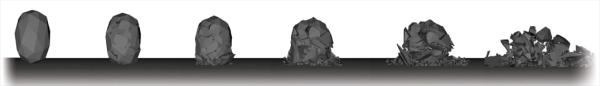
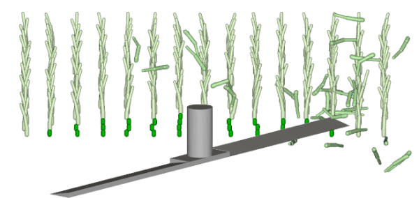
The Particle Shape type you choose and its Composition (see also About Adding and Editing Particle Sets) determines whether or not you are allowed to enable breakage calculations in Rocky, and which kinds of breakage models are available for use.
For rigid particles composed of only a Single Element, only sharp-cornered Solid shapes, such as Polyhedron, Briquette, Faceted Cylinder, and non-concave Custom Polyhedron (imported) particle shapes are compatible with Instantaneous Breakage calculations. The Instantaneous Breakage models available for you to use with these kinds of particle shapes are Ab-T10 and Tavares.
All other rigid, single-element particles are incompatible with breakage models. This includes spherical (Sphere) and rounded-corner Solid shapes (Sphero-Cylinder, Sphero-Polygon, Sphero-Polyhedron), concave-shaped Custom Polyhedrons, and any rigid Fiber and Shell that are composed of only a single element.
In this version of Rocky, any flexible particle composed of Multiple Element (also known as Meshed) are compatible with Discrete Breakage calculations. For Solid shapes, this includes multi-element Polyhedrons and both multi-element convex and concave Custom Polyhedron (imported) particle shapes. For flexible Fiber and Shell, this includes any shape as long as they are composed of Multiple Elements.
The Discrete Breakage models available for you to use with flexible particle shapes include Griffith Energy Criterion, Shear Stress Criterion, Tensile Stress Criterion, Tensile or Shear Stress Criterion, and von Mises Stress Criterion.
In this version of Rocky, there are Instantaneous Breakage models available for rigid particles composed of only a Single Element, and Discrete Breakage models that are specific for flexible particles composed of Multiple Elements. See below for details.
Note: In this version of Rocky, the TBM breakage model is provided as an external module. Refer to the Install an External Module topic for details.
For single-element particles, the Instantaneous Breakage models available are the Ab-T10 and Tavares models. All three models can preserve both mass and volume.
Ab-T10 Breakage Model The Ab-T10 breakage model is based upon the Voronoi fracture particle subdivision algorithm and treats every particle as a single entity that can be broken into fragments instantaneously based upon the breakage force and/or energy values defined.
For more information about how the Ab-T10 breakage model works, refer to the following resources:
The DEM Technical Manual (from the Help menu, point to Manuals and then click DEM Technical Manual)
Tip: For walk-through examples of particle breakage using the Ab-T10 model, review the following resources:
Tavares Breakage Model Like the Ab-T10 model, the Tavares breakage model is based upon the Voronoi fracture particle subdivision algorithm. In this model, however, the breakage energy probability and resulting fragment size distribution are based upon the Tavares et al. (UFRJ) approach. Modeling fracture by low-energy stressing is relevant for the simulation of a number of unit operations in particulate materials processing and handling, where particles are often subject to a complex series of loading events. Tavares' breakage model has been able to describe the progressive growth of crack-like damage (Figure 2) that ultimately leads to the fracture of a particle under stresses significantly lower than those required for breakage in a first event.
Figure 3.164: Illustration showing the effect of weakening due to accrual of damage in repeated loading events
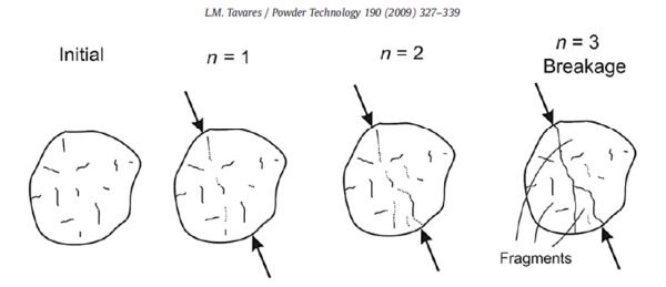
For more information about how the Tavares breakage model works, refer to the following resources:
The DEM Technical Manual (from the Help menu, point to Manuals and then click DEM Technical Manual)
Discrete breakage models can be used only for multi-element (flexible) particles. These types of particles can break only at the joints that otherwise keep the Elements of the particle glued together. Therefore, the fragments resulting from these breakage events will be single Elements or portions of joined Elements.
The Discrete Breakage models available in this version of Rocky are listed below:
Griffith Energy Criterion: This criterion is based on an energy balance that involves the surface energy as a intrinsic property of the joints. This criterion is recommended especially for modeling breakage of flexible solid particles.
Shear Stress Criterion: In this criterion, when the actual shear stress acting on a joint is larger than the specified shear stress limit, the joint will break. This is useful for modeling flexible breakage situations in which the shear or torsion loading conditions are dominant.
Tensile Stress Criterion: In this criterion, when the actual tensile stress acting on a joint is larger than the specified tensile stress limit, the joint will break. This is a useful for modeling breakage of flexible particles subjected mainly to stretching or bending.
Tensile or Shear Stress Criterion: In this criterion, both the actual tensile stress and the actual shear stress acting on a joint are evaluated at the same time and whichever criteria is satisfied first determines when the joint will break. This is useful for modeling breakage in cases in which both the normal and shear stresses are important.
von Mises Stress Criterion: In this criterion, when the (combined) actual tensile stress and actual shear stress acting on a joint is larger than the von Mises stress limit, the joint will break. This is useful for modeling breakage of flexible particles under complex loading conditions.
Tip: Refer also to the DEM Technical Manual. (From the Help menu, point to Manuals and then click DEM Technical Manual.)
Due to the additional calculations involved, a simulation with breakage can be expected to take significantly longer to process. For breakage simulations with very long estimated processing times, consider using Energy Spectra instead. (See also Collecting Data on Contacts and Energy Spectra.)
Limitations: Breakage calculations are not currently compatible with the following settings and functions:
Coarse Grain Modeling. (See also About Physics Parameters.)
Any spherical or rounded-corner Solid particle shapes, including Spheres, Sphero-Cylinder, Sphero-Polygon, and Sphero-Polyhedron particle shapes. (See also About Adding and Editing Particle Sets.)
Any imported Custom Polyhedron particle shapes that are concave and composed of only a single element. (See also About Defining and Importing Custom Particle Shapes.)
Any Shell particle shapes composed of only a single element.
Any Fiber particle shapes composed of only a single element.
For projects processed in older versions (prior to Rocky v4): - Particles Time Selection. (See also About the Particles Time Selection User Process.) - Particle Tagging, including Divisions Tagging. (See also About Particle Tagging.) - Residence Time Property. (See also About Properties.)
If want to save for restart purposes a partially processed simulation with breakage enabled, be aware that any fragments that were in the simulation at the time you save the copy will not be present in the copied version due to incompatibilities between the features. (See also Save a Copy of a Partially Processed Simulation for Restart Purposes.) Note: If you choose to restart processing a copy of a breakage simulation with active fragments at the time of saving, even though no fragments will be present at the initial output time, breakage should work as usual for the new Outputs that are processed thereafter.
When analyzing the Particle Properties of your completed breakage simulation (see also About Properties), be aware that the Impact Specific Energy values you display for particles that are capable of breaking may be inaccurate. This is because Rocky treats differently the storage of energy values for these types of particles only. Note also that this exception does not include broken fragments that are close to the minimum size, as these are considered non-breakable and, therefore, will display the correct Impact Specific Energy values.
What would you like to do?
If the existing particle shapes that come with Rocky do not meet your needs, you can define and import custom particle shapes to use within your simulations. For example, you can achieve a model of a real-world object by using a 3D scanner, or you can design one using a CAD tool like Ansys SpaceClaim. Nearly any kind of shape can be supported in Rocky: convex, concave, perforated, closed, open, and more.
There are three categories of custom particle shapes that can be imported into Rocky:
Custom Fiber particles, which are defined in a text or spreadsheet file.
Custom Shell particles, which are defined in an .stl file.
Custom Polyhedron (Solid) particles, which are defined in an .stl file, and can be categorized as either Convex or Concave. It is these Solid particles that are the best candidates for scanning using a 3D scanner.
Note: Different shapes types have different capabilities in Rocky. Refer to Rocky Particle Shapes and Capabilities for specifics.
See also About Adding and Editing Particle Sets.
To import Custom Shell and Custom Polyhedron (Solid) particles, Rocky needs an .stl file. One way to get that .stl file is to use a CAD program, such as Ansys SpaceClaim, to define your shape and then save the geometry as an .stl file. (See also Appendix F: Save Geometries as XGL, STL, or DXF Files.)
Tip: It is recommended that especially for Shell particle shapes, you do not re-import into Rocky rendered shapes that have been previously exported out of Rocky. (See also Export a Particle Shape to an STL File.) This is because after you import your original Shell shape, Rocky turns that 2D shape into a 3D shape in order to calculate the thickness value, and this 3D aspect is retained when you export the rendered shape out of Rocky. Because Rocky will except only an empty 2D shape when importing Shells, it will not recognize the (now 3D) exported shape as such and will instead want to import it as a solid 3D shape. To avoid this issue, export the Imported Shape instead.
How you design your Custom Polyhedron shape determines whether Rocky will categorize it as a Convex or Concave shape after import. Convex shapes will have no dents or hollows formed by its triangle faces. If Rocky detects even the smallest dent or hollow in the imported .stl, it will categorize that shape as concave-whether that was your intention or not.
Rocky will notify you of this detection via a Convert to Convex? message (Figure 1) that will display after import.
If you are satisfied with the shape being treated as concave, then you can choose the first option on the Convert to Convex? message.
If you still want your shape to be treated as convex, however, you will either need to have Rocky re-draw the shape so that it meets the convexity requirements, or you will need to re-draw and re-import the shape yourself. To do the former, you simply need to select the second option on the Convert to Convex? message. Rocky will use a convex hull algorithm to convert the shape for you.
Tips:
To see a walk-through example of importing a Custom Polyhedron particle shape, review Workshop 09 - Tablet Coater.
To learn more about how Rocky categorizes and calculates convex and concave shapes, refer to the DEM Technical Manual. (From the Rocky Help menu, point to Manuals, and then click DEM Technical Manual.)
Besides designing your Custom Polyhedron particle shape in a CAD program, you can also use a 3D scanner to convert your real-life object into an .stl file that you can then import into Rocky, as shown in Table 1.
Table 1: Typical scenario for scanning a real-world particle shape and importing it into Rocky
|
|
|
|
1. A real-world particle-such as this rock-is scanned on a 3D scanner | 2. The scanned particle is saved as a 3D model (.stl file) | 3. The .stl file is imported into Rocky as a Custom Polyhedron particle shape | 4. A Rocky simulation is conducted using the new custom particle shape |
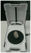


Unlike Custom Shell and Custom Polyhedron (Solid) shapes, Custom Fiber shapes are defined in a text file (Figure 2) or spreadsheet file (Figure 3) (see also File Types and Folders in Rocky).
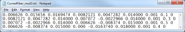
Fiber shapes are made up of separate but connected Segment. The location and characteristics of each Segment are defined in the Custom Fiber's definition file, which contains:
the coordinate location of the Segment's starting and ending nodes
the Segment's diameter (in meters)
an (optional) multiplier of the Young's modulus for the Segment, which is used to define a custom fiber with nonuniform flexibility
an (optional) parameter for turning the Fiber into a frozen Fiber. This works by defining one or more "frozen" Segments, which when used for multi-element (flexible and/or discrete-breakable) particles (see also About Adding and Editing Particle Sets) combined with Custom Inputs (see also About Adding and Editing Particle Inputs), allows the frozen portion of the fiber to "stick" to a certain location and have only the unfrozen portions of the fiber respond to interactions from other objects in the simulation. This can be useful for simulating a field of individual grass blades, for example. Important: This feature works only when the Custom Fiber is composed of multiple elements. (The Particle set's Composition parameter must be set to Multiple Elements.)
Each individual Segment making up the Fiber shape is defined in a separate row according to the following format:
x1,y1,z1,x2,y2,z2,diameter,k_multiplier,frozen,tag
Where:
(x1,y1,z1)represent the Segment's starting nodal coordinate location (in meters)(x2,y2,z2)represent the Segment's ending nodal coordinate location (in meters)diameteris the diameter (in meters) of the indicated Segment(optional)
k_multiplieris the Young's modulus multiplier for the indicated Segment Note: This Young's modulus multiplier is referred to as M in the DEM Technical Manual. (From the Help menu, point to Manuals, and then click DEM Technical Manual.)(optional)
frozenindicates whether Segment will be treated as frozen (1) or unfrozen (0)(Modules Only) tag: this column will only be used with modules that models the custom joint behavior.
Notes:
Values can be separated by spaces (text files only; Figure 2) or commas (spreadsheet files only; Figure 3).
For spreadsheet files only, the first row can be a header row, but this is not required (Figure 3).
Any lines that begin with a number sign (#) (also known as a pound sign or hashtag) will be ignored.
If left undefined, Rocky will treat
k_multiplieras 1 andfrozenas 0.
For example, to create the four-segmented fiber in Figure 3, the coordinate location for the node that starts the first Segment is entered on the row beneath the header (yellow), followed immediately by the coordinate location of the node that ends the first Segment (green), followed by its equivalent diameter (blue)-all in meters-followed by the Young's modulus multiplier (orange), and frozen indicator (gray).
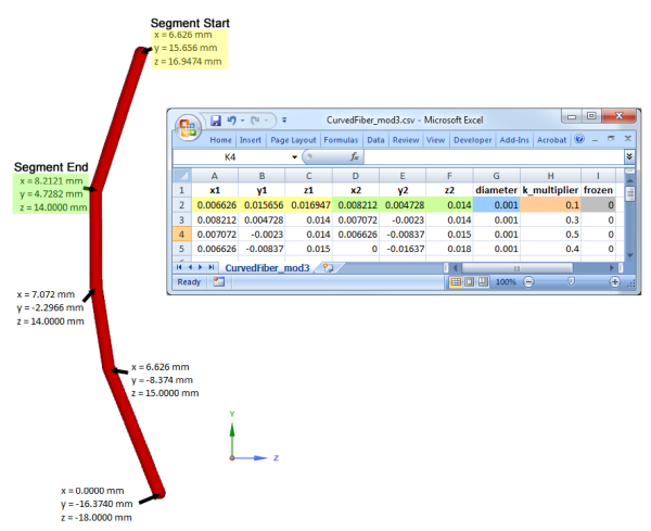
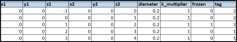
The third row defines the starting and ending node locations for the second Segment in the fiber, and so on. In this way, you can create a wide variety of different segmented shapes.
Important: To ensure predictable results when simulating a custom fiber with Segments that cross, design the fiber so that it includes a node at the desired crossing point. For example, when designing a + (plus) shaped particle whose two Segments cross at their center points, ensure that you include a node in the center of the shape by creating four separate entries in your definition file rather than two.
See also the Flexible custom fibers section in the DEM Technical Manual. (From the Help menu, point to Manuals and then click DEM Technical Manual.)
Important: The complexity of the shape you import has an impact on the overall simulation time so it is important that you aim for as few triangles (or, in the case of Custom Fibers, nodes) in your design as possible that still results in a uniform mesh with good shape representation (see Figure 4). The finer the mesh of your shape, the longer it will take for your simulation to complete.
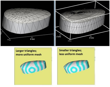 Figure 4 : Shape mesh comparison: The shape on the left has good
meshing and will process faster.
Figure 4 : Shape mesh comparison: The shape on the left has good
meshing and will process faster.
When you choose to import a custom particle shape, you will first be asked to select the shape file you want to use, and will then be asked to verify the import units and scaling criteria (Figure 4).
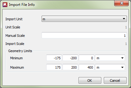
By default, Rocky will import the file as the original size specified in the .stl or .txt file but you can scale the particle down or up as you wish. Note: How you choose to size and scale your particle shape upon import affects how the particle size will be displayed in the Particles Details window only when Original Size Scale is selected on the Size tab for Size Type.
Use the table below to understand the various import parameters you can set for your custom particle shapes.
Table 1: Options on the Import File Info dialog
Setting | Description | Range |
|---|---|---|
Import Unit | Enables you to change the units of the imported shape. | Various units of length |
Unit Scale | Displays the unit scale based upon the Import Unit set. For example, if Import Unit is left as the default value, the Unit Scale will be 1. | Automatically determined |
Manual Scale | Enables you to manually adjust the scale by any factor you want. Leaving the value at 1 will have no additional affect upon the scale. | All values |
Import Scale | Displays the final import scale based upon the Manual Scale and Import Unit values set. For example, if both those options are left as the default values, the Import Scale will be 1. | Automatically determined |
Geometry Limits | ||
Minimum | The minimum coordinates (in X Y Z format) of the particle's geometry. | No limit |
Maximum | The maximum coordinates (in X Y Z format) of the particle's geometry. | No limit |
What would you like to do?
Learn more About Adding and Editing Particle Sets
Learn more about Rocky Particle Shapes and Capabilities
See Also:
From the Data panel, right-click Particles, and then click Create Particle. A new Particle set is listed under Particles in alphabetical (case-sensitive) order.
Select the Particle set you just added, and then from the Data Editors panel, find the Shape list and do one of the following:
From the Select file to import dialog, locate and select the file you want to use, and then click Open.
From the Import File Info dialog, choose the unit and scaling options you want, verify the resulting Geometry Limits, and then click OK.
If you are importing a Custom Polyhedron shape and happen to see the following Convert to Convex? message, select one of the following options, and then click OK:
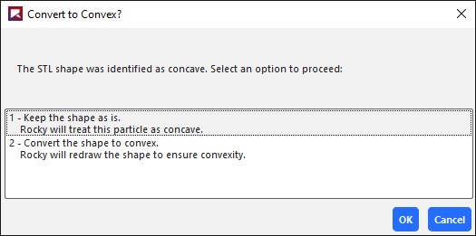
If you want Rocky to calculate the shape as a concave shape, select the 1 - Keep the shape as is option.
If you want Rocky to re-draw your shape so that it qualifies as convex and can be calculated as such, select the 2 - Convert the shape to convex option.
Click the View button to see a 3D view of the largest particle in the Particle set in a Particle Details window. Tip:Use the mouse to rotate, pan, and zoom the image, just like you would in a 3D View window. (See also Use the Mouse, Keyboard, or Toolbar to Change a 3D View.) Also, use the options on the Coloring tab to change the options for Edges and/or Faces (see also About Using the Coloring Tab to Change a 3D View.)
Continue to set up your Particle sets as you normally would. (See also Add and Edit Particle Sets.)
Note: To choose a different file to use for your Particle set, from the Shape sub-tab click Load File, and then follow steps 3-7 above.
Tip: It is recommended that especially for Shell particle shapes, you do not re-import into Rocky rendered shapes that have been previously exported out of Rocky. (See also Export a Particle Shape to an STL File.) This is because after you import your original Shell shape, Rocky turns that 2D shape into a 3D shape in order to calculate the thickness value, and this 3D aspect is retained when you export the rendered shape out of Rocky. Because Rocky will except only an empty 2D shape when importing Shells, it will not recognize the (now 3D) exported shape as such and will instead want to import it as a solid 3D shape. To resolve this issue, export the Imported Shape instead.
See Also:
From the Data panel, right-click Particles, and then click Create Particle. A new Particle set is listed under Particles in alphabetical (case-sensitive) order.
See Also:
From the Data panel, under Particles, click the name of the Particle set you want to modify. The parameters for the Particle set become active in the Data Editors panel.
From the Data Editors panel, modify the parameters as you want.
Tip: To see a detailed 3D view of your particle shape, click the View button.
See Also:
A Particles Details window is where you preview the shape you defined in your Particle set. If you have set collision statistics to be collected during processing, it is also where you will view the details of this data on a representative particle.
Like other types of Rocky windows, you are able to define how the window and the items within it appear and function on screen. After you set up your Particles Details windows, you can choose to reuse the zoom, rotation, and pan settings in another window by saving and applying a Custom Camera Preset. You can also use the Particles Details window as a basis for creating an animation of the Intra-particle Collision Statistics that were collected during the simulation.
What do you want to do?
See Also:
A Particles Details window is where you preview the shape you defined in your Particle set (Figure 1).
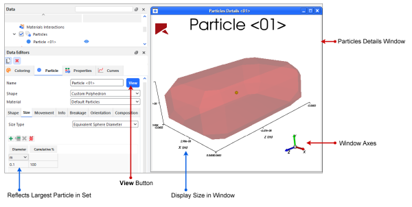
Note: The Geometric Center for a particle is represented in the Particles Details window as a yellow dot.
In addition, if you have set collision statistics to be collected during processing (see also About Collision Statistics for Particles), it is also where you will view the details of this data on a representative particle (Figure 2).
Figure 3.171: Particles Details window overview when used to view collision statistics after processing
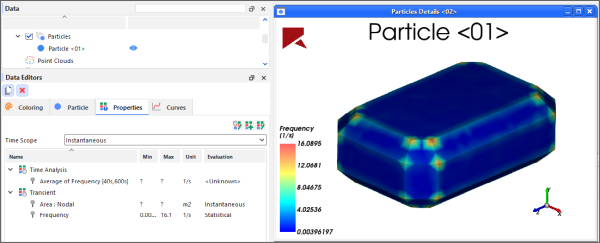
As with 3D View windows, you can use the data shown in the Particles Details window as a basis for creating an animation of the collisions results.
In both cases, you can open this window from the View button on the Particles tab of the selected Particle set (Figure 1).
In this version of Rocky, the preview reflects the size of the largest particle in the selected Particle set. (See also the Size Tab section of the About Adding and Editing Particle Sets.)
Notes:
In order to see the collision statistics, please remove the transparency of the particle.
When displaying particles at a very small scale, there can be display issues related to rendering and lighting. (See also Parts of my particle disappear or appear cut off.)
As with other windows in Rocky, there are various ways you can change what appears in a Particles Details window, including fonts, overlays, background colors, and grid lines.
What do you want to do?
From the Data panel, under Particles, click the name of the Particle set you want to preview. The parameters for the Particle set become active in the Data Editors panel.
From the Data Editors panel, on the Particle tab, click the View button. A new Particles Details window appears in the Workspace showing the selected particle shape in 3D.
Tips:
To show the exact size of an imported shape within the Particle Details window, use the Original Scale Size for Size Type and set the biggest size to 100%.
You can change the look of the Particles Details window in ways similar to a 3D Window. (See also Change a Particles Details Window.)
Note: The window will automatically update when the selected Particle Set's parameters change.
See Also:
There are several ways you can change what you see in the Particles Details window once you have created it, as explained below.
Change the level of zoom or rotation of the Particle by using your mouse, keyboard, or the camera options on the visualization toolbar.
Change the display of the Particle through the Coloring tab on the Data Editors panel.
Change the look of the window display through the Window Editors panel, including changing the default text overlay or adding a logo or image to the display.
When showing a Property after particle collisions have been collected, you can change the display of the colored legend by modifying the Color Scales for the Property you are displaying.
Change the display of the window axes through the top-most "root" Particles Details category on the Windows Editors panel.
What would you like to do?
Learn more about Using the Mouse, Keyboard, or Toolbar to Change a the View
Learn more about Using the Coloring Tab to Change a Particles Details Window
Learn more about Using the Window Editors Panel to Change a Particles Details Window
Learn more About Color Scales
Learn more About Using the Window Editors Panel to Change the Window Axes Displays
See Also:
Learn more About Particles Details Windows
From the Window Editors panel, you can modify just the selected Particles Details window the change the background color, font color/sizes, text and image overlays, and synchronize the Timesteps displayed when two or more view windows are open. You may also adjust the axes display settings for all the windows in your project.
What would you like to do?
See Also:
When you use the Window Editors panel to change the selected Particles Details window, you have the ability to change how items in the window appear on the screen. These items include background color, font color/sizes, and text and/or image overlays (Figure 1). You can also change how multiple windows of the same type respond to changes in Timesteps.
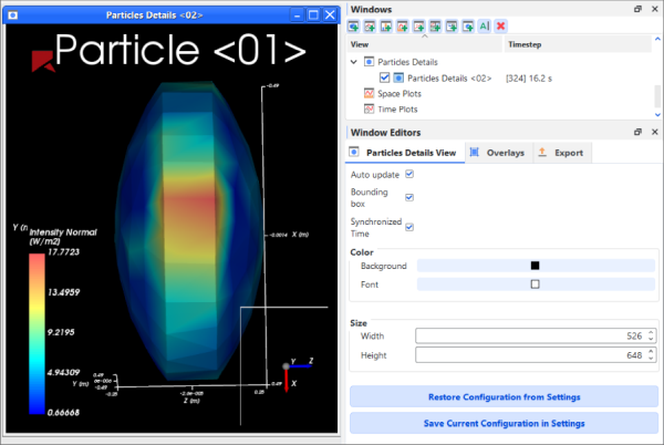
Tips:
You can also use Rocky Preferences to change the background color and fonts for all the Particles Details windows in your project, not just the selected one. (See the "Preferences for Windows Properties" section in the About Setting Global Preferences topic.)
You can also change the window axes display for all windows in your project, including Particles Details windows. (See also About Using the Window Editors Panel to Change the Window Axes Displays.)
In this section, we will cover only the items on the Particles Details View tab and the Overlays tab. Note: The Export tab will be covered in the About Exporting Data and Images Out of Rocky topic.
You use the Particles Details View tab on the Window Editors panel to change how the window appears and how the data displayed within it is updated. These options include changing display items like the background color; labels, lines, and axes colors; color scale label sizes; and window height and width. In addition, you can choose to show or hide the Bounding box, which displays measurements illustrating the simulation boundaries; use Auto update to enable or prevent the view from being updated when data affecting it is changed; or choose to have multiple views updated with the same Timestep by using Synchronized Time.
You use the Overlays tab on the Window Editors panel to change the default text or add image overlays. By default, the text overlay includes the name of the Particle set that you are previewing in the window, but can be changed or removed. Text overlays to include your own custom text or can include Keywords that will show project data, and Input/Output variables, directly on your window view. Image overlays can include company or association logos, photos of real-world equipment, or any applicable image that compliments your simulation. Adding these kinds of overlays are especially useful for generating videos and images from your simulation.
See the images and table below to understand more about how you can use the Window Editors panel to change the selected Particles Details window.
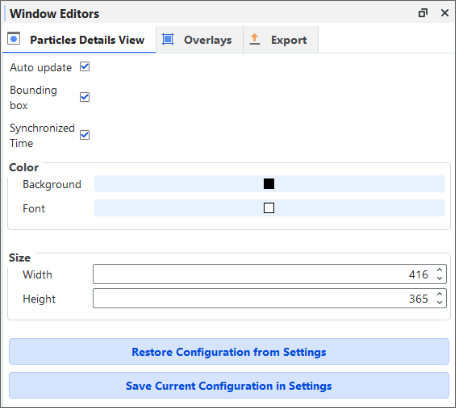
Figure 3.174: Initial Overlays tab options on the Window Editors panel showing default Particle Set text
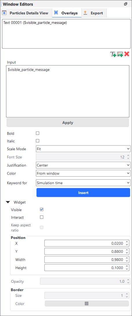
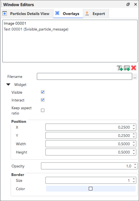
Particles Details View tab options on the Window Editors panel
Setting | Description | Range |
|---|---|---|
Auto update | When enabled, any change made to the display settings of the selected Particles Details window or to the particle shape displayed, will be updated in the Particles Preview window automatically. Because automatically updating the window with each separate change can be computationally intensive, you can clear this option to have all calculated items and more computationally intensive display options remain unchanged in the window until you enable Auto update again. Tip: You will know when the calculations in a Particles Details window are not being updated when you see a thick red border around the window. | Turns on or off |
Bounding box | When enabled, displays measurements illustrating the simulation boundaries in the selected Particles Details window. | Turns on or off |
Synchronized Time | When enabled and the window (or any other window with this checkbox enabled) is selected, the details shown in this (and any other Synchronized Time) window will be updated when the current Timestep is changed on the Time toolbar. (See also About the Time Toolbar).When cleared and the window is selected, only this window will be updated when the current Timestep is changed on the Time toolbar. Tip: To keep the Timestep synchronized between multiple Particles Details or other 3D windows, ensure each window has this option enabled. | Turns on or off |
Color Background | Enables you to change the color that appears behind the particle shape in the Particles Details window. | Options limited by the choices in the Select Color dialog |
Color Font | Enables you to change the color of the labels, borders, and axes lines displayed in the Particles Details window. | Options limited by the choices in the Select Color dialog |
Size Width | Enables you to numerically change how wide the selected window is. Useful in cases where you need exact dimensions for image consistency. | Whole positive values between 123 and 5000. |
Size Height | Enables you to numerically change how tall the window is. Useful in cases where you need exact dimensions for image consistency. | Whole positive values between 0 (zero) and 5000. |
Restore Configuration from Settings | Clicking this button replaces the values set on the tab with the ones that have been saved to the (internal) Rocky Settings folder. (See also Rocky File Types and Folders). | (Button selection) |
Save Current Configuration in Settings | Clicking this button overwrites the values that have been saved to the (internal) Rocky Settings folder with the ones currently set on the tab. (See also Rocky File Types and Folders). | (Button selection) |
Overlays tab options on the Window Editors panel for Text and Image Overlays
Setting | Description | Range |
|---|---|---|
Text Overlays Only | ||
Input | This box displays the text, phrase, or keyword that you want overlaid onto the selected window. It can be static text that you type in, can be dynamic text by using the Keyword for list, or can be a combination of both. | No limit |
Bold | Enables the selected text overlay to appear bold in the window. | Turns on or off |
Italic | Enables the selected text overlay to appear italic in the window. | Turns on or off |
Scale Mode | Determines how the text in the selected overlay scales in relation to its Font Size, the sizing box that surrounds it, and size of the window itself. Specifically:
| Font Size; Fit; Scaled Font Size |
Font Size | When Font Size or Scaled Font Size are chosen for Scale Mode, this sets the size of the text in the selected overlay. | Whole positive values |
Justification | Aligns the selected text horizontally in the overlay box. Tip: This feature is really only useful when you several lines of text. Use hard returns (press the Enter key) to force text to the next line. | Left Center Right |
Color | Enables you to indicate from what location the font color overlay text will be taken. Specifically:
| From window Custom |
Keyword for | Enables you to enter Rocky-specific placeholder values for data and settings that pertain to your simulation. As your simulation processes or as you change your timestep, and assuming you have selected Auto update on the (Window Type) tab (see Table 1 above), these values will be updated automatically in the text overlay. In addition to the items explained below, if you have defined any Input or Output Variables (see also About Defining and Using Input Variables and About Defining Output Variables), these will be listed here as well. See below for more information on keywords.
Tip: If you find that it takes too long to update the text displayed when changing Timesteps or other data, consider clearing the Auto update checkbox on the (Window Type) tab until your changes are complete. (See Table 1 above.) | Simulation time; Simulation time index; Simulation time value; Study Customer Name; Study Description; Study N. Particles; Study Name; Visible Particle Message |
Image Overlays Only | ||
Filename | This is the location and file name of the image you want overlaid onto the selected window. | .bmp .jpg .png .pnp |
Widget (both Text and Image Overlays) | ||
Visible | When enabled, shows the selected overlay in the window. When cleared, it hides the overlay. | Turns on or off |
Interact | When enabled, allows you to move and resize the selected overlay. When cleared, it locks the size and position. | Turns on or off |
Keep aspect ratio | When enabled, locks the aspect ratio of the sizing box surrounding the overlay so that when you resize it, the shape of the box is maintained. When cleared, you may change the shape of the sizing box surrounding the overlay. Note: The shape of the sizing box has no real effect upon the display of the overlay. No matter the shape, Rocky will automatically maximize the size of the content to fill it. | Turns on or off |
Position | X | For the selected overlay, this defines the X-position of the sizing box's lower left corner normalized in relation to the window size. A value of zero (0) is equal to the left window border and a value of 1 is equal to the right window border. | 0-1 |
Position | Y | For the selected overlay, this defines the Y-position of the sizing box's lower left corner normalized in relation to the window size. A value of zero (0) is equal to the lower window border and a value of 1 is equal to the upper window border. | 0-1 |
Position | Width | For the selected overlay, this defines the width of the sizing box normalized in relation to the window size. A value of 1 is equal to the full width of the window. | 0-1 |
Position | Height | For the selected overlay, this defines the height of the sizing box normalized in relation to the window size. A value of 1 is equal to the full height of the window. | 0-1 |
Opacity | Enables you to adjust the transparency of the overlay. The higher the value, the more opaque the overlay appears. The lower the value, the more transparent. | 0.0 - 1.0 (Values limited by UI) |
Border Size | Enables you to increase the thickness of the sizing box that surrounds the overlay. | Whole positive values including 0 (zero) |
Border Color | Enables you to change the color of the sizing box that surrounds the overlay. | Options limited by the choices in the Select Color dialog. |
What would you like to do?
See Also:
Ensure the Window Editors panel is visible. (From the View menu, click Window Editors.)
From the Workspace, select the Particles Details window that you want to change. (See also Preview a Particle Shape in 3D.)
From the Window Editors panel, select the Overlays tab and then do one of the following:
To add a new image, do all of the following:
Click the Add image overlay button. A new Image entry appears in the Overlays list.
Under Input click the … button next to Filename.
From the Load File dialog, navigate to and select the image file you want, and then click Open.
The location of the file you selected is displayed in the Filename box and the Image entry is appended with the file name. The image you selected appears in the selected window.
To edit an existing image, under Input, select the entry representing the image that you want to change.
Do any or all of the following: - To move the image, use your mouse to click the center of the image and drag it to a new location on the window. - To change the size of the image, click the image border in the window, and then drag to resize as desired.
Note: While the Keep aspect ratio (under Widget) setting will allow you to change the shape of the sizing box that surrounds the image, it will not affect the size of the image itself. No matter the shape of the sizing box, Rocky will maximize the image size to fill it.
To hide the image from the window, under Widget, clear the Visible checkbox.
To lock the size and position of the image, under Widget, clear the Interact checkbox.
To change how transparent the image is, under Widget, edit the Opacity value. Tip:Click away from the Opacity box to have your changes applied to the window.
To change the appearance of the box bordering the image, choose what you want under Widget for Border Size and Border Color.
To remove the image from the selected window, click the Remove overlay button.
See Also:
Ensure the Window Editors panel is visible. (From the View menu, click Window Editors.)
From the Workspace, select the Particles Details window that you want to change. (See also Preview a Particle Shape in 3D.)
From the Window Editors panel, select the Overlays tab and then do one of the following:
To edit an existing text overlay, select the name of the text you want to change from the list at the top of the panel.
To add a new text overlay, click the Add text overlay button. A new Text entry appears in the Overlays list at the top of the panel.
Do any or all of the following:
To enter your own text, under Input, place your cursor directly into the Text entry and then remove and add text as you like using your keyboard.
To have Rocky automatically display simulation-related text, including simulation time or study name, in the Input box, place your cursor where you want the text to be inserted, choose what you want from the Keyword for list, and then click Insert. The placeholder text appears in the Input box. Tip:To see the text replaced with real values on the selected window, click Apply.
To change how the text is displayed in the window, edit the Bold, Italic, Scale Mode, Font Size, Justification, and Color options as you want. (See also About Using the Window Editors Panel to Change the Selected Particles Details Window.)
To move the text, do one of the following:
Use your mouse to click the center of the text box and then drag it to a new location on the window.
Under Widget, use the Position options for X and Y.
To change the size and shape of the text box, do one of the following:
Click the text box border in the window, and then drag the border to resize or reshape the text box.
Under Widget, use the Position options for Width and Height.
Note: While the Keep aspect ratio (under Widget) setting will allow you to change the shape of the sizing box that surrounds the text, it will not affect the size of the text itself. No matter the shape of the sizing box, Rocky will maximize the text size to fill it.
To hide the text from the window, under Widget, clear the Visible checkbox.
To lock the size and position of the text box, under Widget, clear the Interact checkbox.
To change how transparent the text is, under Widget, edit the Opacity value. Tip:Click away from the Opacity box to have your changes applied to the selected window.
To change the appearance of the box surrounding the text, choose what you want under Widget for Border Size and Border Color.
To remove the selected overlay from the window entirely, click the Remove overlay button.
See Also:
Ensure the Window Editors panel is visible. (From the View menu, click Window Editors.)
From the Workspace, select the Particles Details window that you want to change. (See also Preview a Particle Shape in 3D.)
From the Window Editors panel, select the Particles Details View tab and then change the options you want.
Tips:
You can also open the Window Editors panel for a window by right-clicking an empty space within the Particles Details window (for example, the background behind the particle), and then clicking Settings.
You can also use Rocky Preferences to change the background color and fonts for all the Particles Details windows in your project, not just selected one. (See the "Preferences for Windows Properties" section in the About Setting Global Preferences topic.)
To reuse in future projects the settings you made to this tab, click the Save Current Configuration in Settings button.
To apply settings you have already saved (either by previously using the Save Current Configuration in Settings button or by saving selections within the Preferences dialog) to this tab, click the Restore Configuration from Settings button.
See Also:
The Coloring tab, located on the Data Editors panel for all simulation entities and User Processes, enables you to change the colors and data attributes of the particle shape being displayed in a Particles Details window. Faces, edges, and nodes can be shown or hidden; displayed in solid colors; or colored by a Property property of your choice.
In addition, when showing the results of Collisions Statistics, the Coloring tab also enables you to modify the limits, units, and legend options for the color scales used in your Particles Details windows.
What would you like to do?
See Also:
Using the options on the Coloring tab is one way you can change what is displayed in a Particles Details window for the Particle set that you want to change. Visualization options for the Faces, Edges, and Nodes can be modified with the Coloring tab.
When analyzing the results of Intra-particle Collision Statistics, you may from the Coloring tab also adjust the Color scales for the Property you are viewing. However, the options presented are quite different than the ones explained below. For more information, see also About Color Scales.
See the image and table below to help you understand how to use the Coloring tab to change a view for selected entity.
Figure 3.176: Example Coloring tab in the Data Editors panel showing Particle Set parameters for a Particles Details window
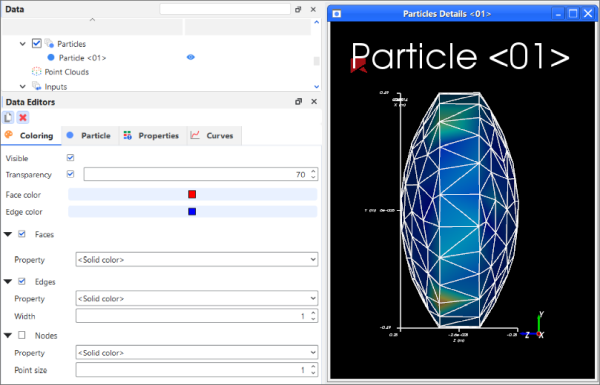
Table 1: Coloring tab parameter options for Particle sets in the Particles Details window
Setting | Description | Range |
|---|---|---|
Visible | When enabled, shows the selected entity in the active view window. Note: This is the same as using the Data panel eye icon. (See also Show/Hide Components by Using Eye icons and Checkboxes). | Turns on or off |
Transparency | Enables boundaries to be drawn transparently in the selected view window. A value of 0 (zero) makes the faces completely solid or opaque. A value of 100 makes the faces completely transparent or hidden. | Turns on or off; 0-100 |
Color | When Faces, Edges, and/or Nodes are selected and the Property is <Solid Color>, this enables the selected display type to be colored in the one solid color chosen. Note: For Faces, Transparency options affect how opaque this color appears in the view. | Options limited by the Select Color dialog |
Faces | Enables the entire surface of the entity to be visible and affected by the various Faces coloring options. | Turns on or off |
Property | Three separate lists under Faces, Edges, and Nodes respectively provide properties and other color options that apply to the display type within which the list is contained. Specifically:
| <Solid color>; List of properties automatically generated from the Properties tab |
Edges | Enables only the edges bordering the components making up the entity boundaries visible and affected by the various Edges coloring options. | Turns on or off |
Width | When Edges is selected, this changes the thickness of the lines used to draw the borders. Entering 1 will provide the narrowest line. | Positive values |
Nodes | Enables the points marking the intersections of the entity's individual components to be visualized as dots and affected by the various Nodes coloring options. | Turns on or off |
Point Size | When Nodes is selected, this changes the size of the dots used to draw the nodes. Entering 1 will provide the smallest dot. | Positive values |
What would you like to do?
See Also:
From the Workspace, select the Particles Details window containing the *Particle set* to which you want to apply changes. (See also Preview a Particle Shape in 3D.)
From the Data panel, under Particles, select the Particle set you want to change.
From the Data Editors panel, select the Coloring tab, and then change the settings you want. The changes you make are shown automatically in the selected Particles Details window.
See Also:
From the Data panel, under Particles, right-click the name of the Particle set you want to remove, and then click Remove Particle.
See Also:
In cases where you need to make use of your particle shape outside of Rocky, you may choose to export your rendered shape (any particle shape) or your originally imported shape (Custom Particle Shapes only) to an .stl file. Doing so enables you to select the size and units you want to use when exporting (Figure 1).
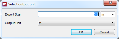
From the Data panel, under Particles, right-click the Particle set containing the shape you want to export, point to Export, and then do one of the following:
For default and custom imported particle shapes, click Rendered Shape to export Rocky's current (and perhaps altered) copy of the shape file.
For custom imported particle shapes only, click Imported Shape to export the original (unaltered) file.
From the Select output unit dialog, enter the Export Size, select from the Output Unit list the units you want, and then click OK.
From the Select target STL file dialog, click the drive or folder of the location to which you want to save the file.
In the File name box, enter a name for the file, and then click Save.
Note: If you are wanting to export a rendered Shell shape out of Rocky, be aware that the exported Shell shape will no longer be considered a true Shell (2D) shape due to the thickness Rocky applies to its walls. It is for this reason that it is recommended that you do not re-import a previously exported rendered Shell shape back into the Rocky program.
See Also:
Point Clouds enable you to import a text file containing field data that defines one or more points in space.
Tip: Unless you have enabled an external Module that makes use of Point Clouds, you can skip the Point Clouds part of your Rocky setup.
What would you like to do?
See Also:
In this version of Rocky, the primary purpose of Point Clouds are to support the functionality within custom external Modules whose models require information that varies through all three dimensions of the domain and/or over time.
Tip: Unless you have enabled an external Module that makes use of Point Clouds, you can skip the Point Clouds part of your Rocky setup.
Specifically, Point Clouds enable you to import a text file containing field data that defines one or more static points in space. Moreover, you can load a set of point clouds at once by importing a transient point cloud text file, which specifies the start and end times for individual static point clouds. This data can then be used by Rocky in various ways depending upon the functionality of the external Module making use of the Point Cloud.
(See also About Modules Parameters.)
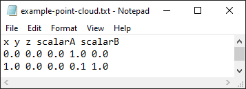
The text file you import for a Static Point Cloud must be formatted in the following way:
The file must be saved as a .txt extension with spaces separating each value. Important: No matter your system's location settings, ensure that you use dots (periods) and do not use commas to indicate decimals in this particular text file.
The first (header) row must contain the names of each value defined.
The first three (required) columns must be
(x, y, z), which together define the coordinate location of the point.The forth (required) column must include a scalar variable. (The variable you include will be dependent upon how the Point Cloud will be used.)
The fifth and subsequent columns (optional) can include additional scalar variables as needed.
The second and subsequent rows define the values for each individual point.
Figure 3.179: Example text file defining the main file of a Transient Point Cloud with three Static Point Clouds.
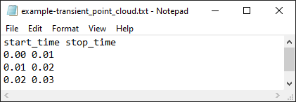
Transient Point Clouds consist of sets of Static Point Clouds that are applied during the simulation following specific start and end times. In order to import a Transient Point Cloud, it is necessary to import a main text file containing the start and end times of each Static Point Cloud that will be then automatically imported to compose the Transient Point Cloud.
The main text file you import for a Transient Point Cloud must be formatted in the following way (see Example text file defining the main file of a Transient Point Cloud with three Point Clouds):
The file must be saved as a .txt extension with spaces separating each value. Important: No matter your system's location settings, ensure that you use dots (periods) and not commas to indicate decimals in this particular text file.
The first (header) row must contain only the start_time and the stop_time names.
The second and subsequent rows define the start time and the stop time values for the Static Point Clouds that you want to be imported.
The start time value in the first row not necessarilly needs to be zero.
The stop time entry in the last row can be empty so the last Static Point Cloud will be enabled until the end of the simulation.
Figure 3.180: Example text files structure to define a Transient Static Point Cloud with three Static Point Clouds.
The Static Point Clouds text files that makes up the Transient Point Clouds must have the same format as the regular Static Point Clouds. (See also About Creating a Static Point Cloud Definition File.)
The Transient Point Cloud files structure must follow these rules (see Example text file defining the main file of a Transient Point Cloud with three Point Clouds):
The main Transient Point Cloud text file and each Static Point Cloud text files must be located at the same folder.
The filename of each of the Static Point Clouds must be the same one used for the main Transient Point Cloud txt file, but adding an index at the end of the filename.
The start and the stop times defined in the main text file rows will be considered to load the Static Point Clouds into the simulation. Each row is related to each Static Point Cloud index, starting from 0.
In this version of Rocky, you can visualize in a 3D View window the individual points defined within your Point Cloud Definition File (Figure 2).

(See also About Using the Coloring Tab to Change a 3D View.)
Use the image and table below to help you understand the settings for a Point Cloud.
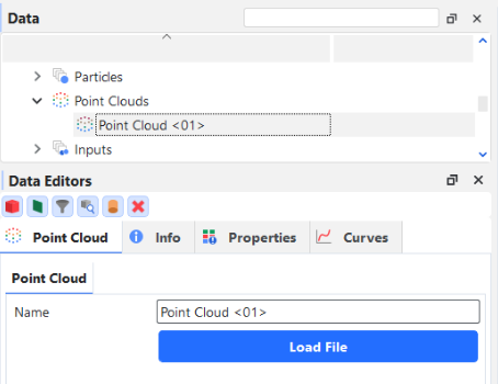
Table 1: Point Cloud parameter options
|
Setting |
Description |
Range |
|---|---|---|
|
Name |
Enables you to specify a unique identifier for the Point Cloud. |
99 character limit |
What would you like to do?
See Also:
Ensure you have enabled an external Module that makes use of Point Clouds.
Tip: If you do not plan to enable an external Module that makes use of Point Clouds, then you do not need to add a Point Cloud to your simulation.
Ensure you have a Point Cloud definition text file that is formatted according to the way Rocky expects. (See also About Point Clouds.)
From the Data panel, right-click Study, select Point Cloud, and then click Create Point Cloud.
From the Data panel, under Point Clouds select the newly added Point Cloud entry.
Note: The Point Clouds entity shows up only if you create a Point Cloud, otherwise it will be hidden from the Study.
From the Data Editors panel, on the main Point Cloud tab, enter a Name and then click the Load File button.
From the Select file to import dialog, navigate to and select the .txt file you want to use, and then click Open.
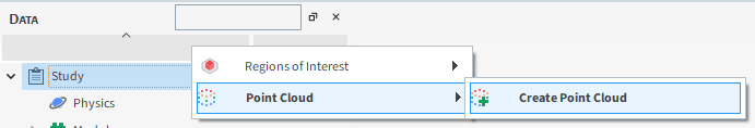
See Also:
From the Data panel, under Point Clouds select the Point Cloud entry you want to change.
From the Data Editors panel, do one of the following:
To edit the Point Cloud, from the main Point Cloud tab, do any of the following:
Enter a different Name.
Click the Load File button and then from the Select file to import dialog, navigate to and select the new .txt file you want to use, and then click Open.
To remove the Point Cloud, click the Remove Point Cloud button.
For the latest Rocky release, the support for Time Periodic was added to the Transient Point Clouds capabilities, enabling to execution of the whole Point Cloud data as periodic, repeating its data respecting the Start and Stop time that is available to configure in the Data Editors.
To edit the Time Periodic for the Transient Point Cloud, from the main Point Cloud tab, do the following
Check the Enable Periodic option in the Data Editors, and then, enter a Start Time and a Stop Time, which will control the times that the Periodic will begin and be finished. Then, the Point Cloud Data will repeat, constantly, respecting the Start-Stop time which were chosen.
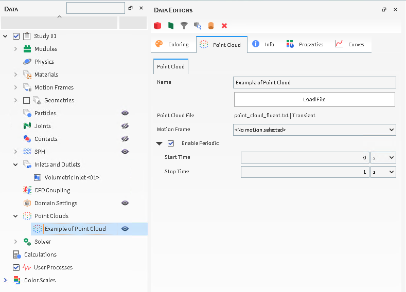
For the latest Rocky release, the support for Motion Frame was also added to Point Cloud capabilities, enabling to move of the Point Cloud data accordingly with the already configured Motion Frame, that can be selected in the Data Editors. This Motion Frame support is available for both Static and Transient Point Cloud data, as well it works with the new Time Periodic supprt.
To edit the Motion Frame for the Point Cloud, from the main Point Cloud tab, do the following
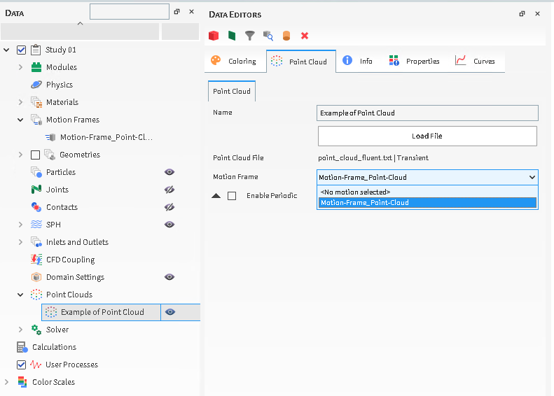
See Also:
The Inlet and Outlets entity on the Data panel is where you specify how and where various particle and fluid sets will be entering (or leaving) your simulation-for example, through continuous injection, volumetric inlet, or custom positioning that you define in a text or spreadsheet file-and get an estimate of how many particles might be released from those inlet locations during the simulation.
What would you like to do?
See Also:
Inlets define how particles or fluids are injected into a simulation. Outlets define the surface(s) where particles or fluids leave the simulation. In this version of Rocky, there are four different inlet methods (Particle Inlet, Particle Custom Inlet, Volumetric Inlet, and Fluid Inlet) and one outlet option. See the sections below to learn more about adding and editing the various kinds of inlets and outlet in Rocky.
The Particle Inlet method enables you to release particles in a continuous or periodic stream from the Entry Point (Surface or Feed Conveyor) that you select (Figure 1).
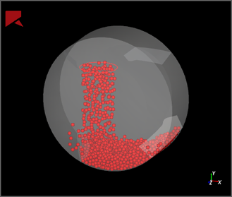
With this method, the size and shape of both the Entry Point and the particles within the set (see also About Adding and Editing Particle Sets), as well as the Mass Flow Rate and particle overlap criteria that that you define (see also About Solver Parameters) all have an effect on the injection speed and relative placement (or "packing") of the particles as they are released.
In addition, you are able to delay or halt particle injection at various times in the simulation.
The Fluid Inlet method enables you to set an inlet of fluid into your simulation. With this method, the temperature of the fluid (if a thermal model is enabled) and the surface that will serve as inlet can be defined. Additionally, you can choose to set the Mass Flow Rate or the Velocity as a boundary condition and be able to delay or halt fluid injection at various times in the simulation.
The Volumetric Inlet method enables you to inject a spheric region of closely packed particles into a simulation all at one time (Figure 2). Alternatively you can use this method to create a region that will be filled with fluid, using the SPH tab.
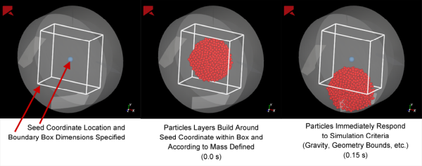
Rocky does this by building layers of particles around a central Seed Coordinate point you specify. These layers continue to build making the sphere bigger until one of two things happens: it either meets the Mass value that you set or it reaches the limits you define-whichever comes first. The limits you define must include a boundary box-the volume of which Rocky uses to limit the particle fill- but can also include the walls or surfaces of one or more boundaries within your simulation.
Choosing to constrain the fill by a geometry (wall or surface) enables you to have the fill build within, around, or through objects, which can be useful in certain situations (Figures 3-4).
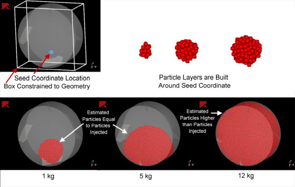
Figure 3.189: Example of a Volumetric Inlet following along the walls of the pipe geometry to which the inlet was constrained
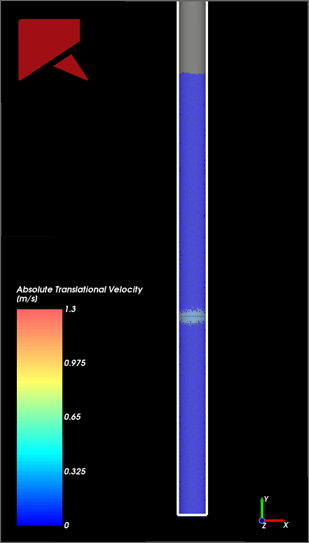
How closely the particles are to each other when they build around the Seed Coordinate (the "gap" between them) is determined by the Gap Scale Factor you set. A default factor of 1 places the particles right next to each other; a factor of 2 places the particles as if they were twice the size, and so on (Figure 5).
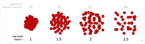
Defining a factor that is too big for your Box bounds will result in fewer particles being injected-as shown in the last example in Figure 5.
Note: Volumetric Inlets require a minimum of 3 particles in order to create the "Seed". You may need to adjust your Mass and other Volumetric Inlet properties to ensure that Rocky can generate enough particles to meet this requirement.
With the Volumetric Inlet method, the size and shape of the particles within the set (see also About Adding and Editing Particle Sets) and the set's Material properties (see also About Modifying Material Compositions)-not to mention the limits and Gap Scale Factor you define-all work together to determine how the Mass you enter translates into the amount of particles to be injected.
While the Volumetric Inlet option serves to provide maximum flexibility with regards to your set up, this complexity can also increase your chances for mistakes. Please review My Volumetric Inlet isn't working right to learn how to avoid the most common pitfalls.
Tip: To see walk-through examples using the Volumetric Inlet, refer to the following Workshops:
Volumetric Inlet for non-spherical shapes considers the biggest distance between two points—i.e., the longest length within the boundaries of the particle—and uses that distance to create a spherical buffer around the particle that exists only during the initial timestep of the injection. This buffer prevents other particles—no matter their orientation—from going inside another particle's buffer. While this strategy prevents overlaps during injection, it can also cause wider "gaps" between some types of particles. As the biggest length of the non-spherical shape increases, the distance between particles (also known as the "gap" between them) increases, and fewer particles are injected during Volumetric Inlet.
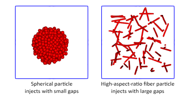
In the illustration shown in Figure 6, spherical particles and high-aspect-ratio fiber particles of the same initial mass and tonnage are injected via separate but identical Volumetric Inlet regions. While the spherical particles are injected closely together, the fiber particles are injected much farther apart due to the spherical buffer required for overlap control. And as a result, the fiber particles reach the limits of the Volumetric Inlet region much sooner, thereby injecting fewer particles.
Tip: For more information about how overlaps are calculated in Rocky, refer to Figure 2.1 in the Rocky DEM Technical Manual.
The Volumetric Inlet for fluids option (available through the SPH tab inside Volumetric Inlet), allows for the injection of fluid in a controlled region. It works in the same fashion as the particle volumetric inlet, including the possibility of using one or more geometries to define the region that will be filled with fluid.
The main difference between the fluid and particle volumetric inlet is that the fluid input parameters are only the fluid mass and temperature (available only if a thermal model is enabled).
If desired, you can combine the usage of the imported geometries and the bounding box to achieve flat surfaces.
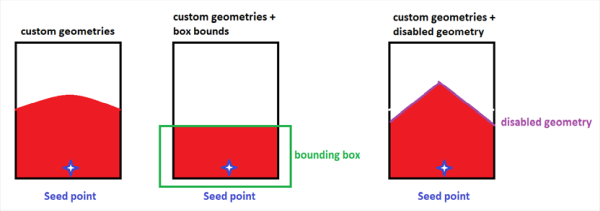
In the first image in the example above, you can see the particle bed that is generated when the walls are used as the imported geometry for the Volumetric Inlet. In the second image, you can see what happens if you use the same imported geometry but add a bounding box that limits the particle generation. As the particles reach the bounding box, Rocky cannot inject more particles, and the surface of the Volumetric Inlet is flat.
If you want to limit the inlet to a surface that is not flat, you can use the following workaround:
Import a geometry representing the profile of your desired top surface-such as the peak used in the third image in the example above.
Set this geometry to be used only the initialization period-which is when the volume fill happens. You can accomplish this by setting the geometries Enable Time to be a very large value that ever be reached in the simulation, such as 999 s.
The Particle Custom Inlet method enables you to position particles in the exact locations, times, amounts, sizes, speeds, and orientations that you want. You accomplish this by specifying certain values in a special definition file that you import into Rocky, and then assign a Particle set to it.
The definition file you create for the Particle Custom Inlet determines when and how particles are placed inside your domain. The resulting spreadsheet can be saved in various formats, such as .csv (Figure 8), .xls, .xlsx (Figure 9), .xlsm, .xlsb, and .odf. (See also File Types and Folders in Rocky.)
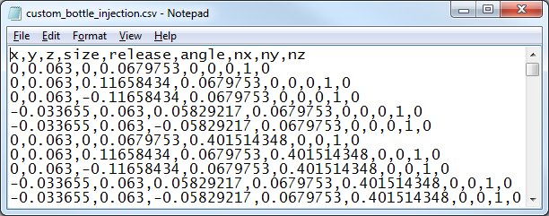 Figure 8: Example of a Particle Custom Inlet definition file showing a .csv file with commas separating the columns
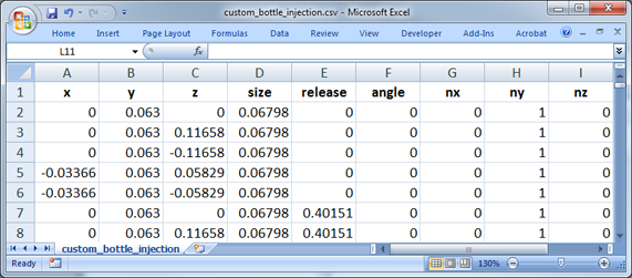 Figure 9: Example of a Particle Custom Inlet definition file shown in Microsoft Excel
Besides accepting only these file types, the other requirements for the definition file are that it is saved so that the values are separated by commas (sometimes called comma delimited or Comma Separated Value files) (Figure 8), and that it is formatted according to the way Rocky expects. Specifically, that the first row must contain the header information of the required and optional columns you are including, and that each individual particle making up the Particle Custom Inlet is defined in a separate subsequent row according to the following format, which is composed of fields that can be defined in any order:
x,y,z,release,size,angle,nx,ny,nz,temperature,ux,uy,uz,wx,wy,wz
These fields are explained in the following table.
Table 3.2: Particle Custom Inlet Definition File Field Definitions
| Field | Type | Definition | Unit | Notes and Tips |
|---|---|---|---|---|
| xyz | Required | Defines the global coordinates of the domain location where the particle will be positioned. | mmm |
|
| release | Optional | The simulation time you want the particle to appear in the simulation. | s |
|
| size | Optional | Defines the Size, Diameter, or Scale Factor of the particle to be released, based upon the Size Type that you defined for the Particle set on the Particle | Size tab. | m |
|
| angle nx, ny, nz. | Optional | Defines the amount of particle rotation (angle) around a unit vector (nx,ny,nz). | rad mmm |
|
| temperature | Required only when the Thermal Model is enabled | Defines the temperature the particle will have at time of release. | K |
|
| ux, uy, uz. | Optional | Defines the initial translational velocity of the particle as it is released. | m/sm/sm/s | |
| wx,wy,wz. | Optional | Defines the initial angular velocity of the particle as it is released. | rad/srad/srad/s |
After the definition file is imported as part of the Particle Custom Inlet process, Rocky will display a summary view of the file contents in a special File Info section (Figures 16-17). Here you can verify the number of particles that have been defined, as well as the minimum and maximum values of the other fields within the file.
When combined with frozen Fibers (see also About Defining and Importing Custom Particle Shapes), Particle Custom Inlets have the added benefit of assigning a Motion Frame (About Creating and Applying Motion Frames) to the injected particles. In these cases, the frozen Segments of the injected fibers will move according to the frame definition. This combination can be useful for simulating a broom, for example.
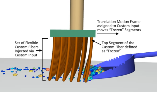
In the example shown in Figure 10, the Particle Custom Inlet defines the exact placement of the flexible Custom Fiber bristles, and the assigned Motion Frame translates the fibers by moving only the frozen top Segment that was defined for the fibers.
Important: For Particle Custom Inlets to work property with Frozen Fibers, all release times in the Particle Custom Inlet
definition file must either be defined as 0 (zero) or the release field itself must be omitted from the file.
Limitations: In this release of Rocky, the three-way combination of a (1) Particle Custom Inlet being defined with (2) Frozen Fibers and also having a (3) Motion Frame assigned to the Particle Custom Inlet is, as a specific combination, incompatible with both Cartesian and Cylindrical Periodic Domains. (See also About Domain Settings Parameters and Particle and Inlet Limitations.)
You can also use the information on the Info tab to get an estimate of how many particles might be released from each inlet during the simulation. (See also About the Info Tab.)
Notes:
For both Continuous Feed and Volumetric Inlet types, the particle estimate does not take into account simulation-specific events such as the inlet being blocked by a moving boundary or by previously-injected particles.
For Volumetric Inlet specifically, the estimate assumes there are no boundary limits to consider, and assumes a Gap Scale Factor equal to 1. This means that if you have set your particle Mass higher than the box and gap you define can contain, the particle estimate on the Info tab will show a higher number than what will actually be injected (Figure 3).
For Particle Custom Inlet specifically, the particle estimate is equal to the Number of Particles value on the Particle Custom Inlet tab.
Before you can process your simulation, you must create at least one particle or fluid inlet and provide either the Mass Flow Rate value (for Fluid or Particle Inlet), Mass value (for Volumetric Inlet), or valid definition file (for Particle Custom Inlet) for at least one Particle set.
If you have enabled one or more external Modules that affect your Inlet or Outlet settings, you might also have a separate Modules sub-tab or separate, module-specific settings that you can define. Refer to the Module's documentation (if provided) for more information. (See also Rocky Simulation Entities that can be Affected by Modules.)
Use the figures and tables below to help you understand the various parameters you can set for inlets.
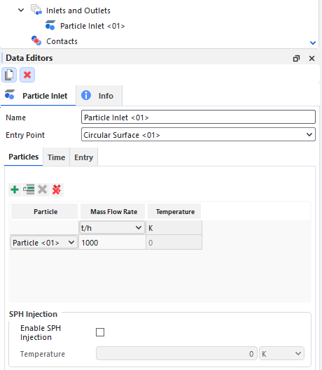
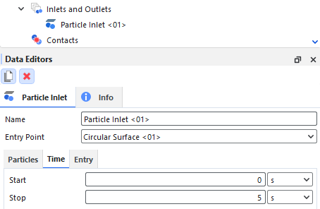
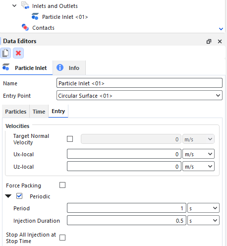
Table 2: Particle Inlet parameter options
|
Setting |
Description |
Range |
|---|---|---|
|
Name |
Enables you to specify a unique identifier for the particle inlet. |
99 character limit |
|
Entry Point |
The Feed Conveyor or inlet from which the particles are released during the simulation. Note: Only one Inlet can be set per Entry Point. Tip: To have multiple Inlets be released from a single location, create multiple Inlets and then define a separate Input per Inlet. |
Any Planar Surface |
|
Particles sub-tab | ||
|
Particle |
The Particle set that you want to enter the simulation from the Entry Point specified. |
Any Particle set specified in the simulation |
|
Mass Flow Rate |
The mass flow rate for the Particle set that you want released from this Entry Point. |
Values above but not equal to 0 ton/h Note: The one exception to this rule is if you want to change the active Inlets after you Save a Copy of a Partially Processed Simulation for Restart Purposes. (See also About Changing Geometries and/or Particles in a Partially Processed Simulation). |
|
Temperature |
When Thermal Model is enabled (see also About Physics Parameters), this is the temperature that all particles in the Particle set will have when released from this Entry point . |
Values above but not equal to 0 K (zero Kelvin) |
|
Enable SPH Injection |
When the check box is enabled, allows for the injection of fluid that fills the space between the particles. |
Turns on or off |
|
Temperature |
The temperature of the fluid that will be inject with the particles (Only available if Enable SPH Injection checkbox and the Thermal Model are enabled). |
Values above but not equal to 0 K (zero Kelvin) |
|
Time sub-tab | ||
|
Start |
The time you want particles to begin releasing from the Entry Point. Note: If you choose to use parametric expressions in this field, know that only the resulting value and not the variables and/or mathematical functions you enter will be retained in any project copies you save for restart purposes. (See also I get a "Links removed" message when I save my project for restart purposes). |
Positive values Tip: Check the Status panel to ensure that any variables or mathematical functions you might use results in valid values. (See also Double-Click the Status Panel to Jump to the Appropriate UI Location). |
|
Stop |
The time you want particles to stop releasing from the Entry Point. Note: If you choose to use parametric expressions in this field, know that only the resulting value and not the variables and/or mathematical functions you enter will be retained in any project copies you save for restart purposes. (See also I get a "Links removed" message when I save my project for restart purposes). |
Positive values Tip: Check the Status panel to ensure that any variables or mathematical functions you might use results in valid values. (See also Double-Click the Status Panel to Jump to the Appropriate UI Location). |
|
Entry sub-tab | ||
|
Target Normal Velocity |
When selected, enables you to set the normal speed of the particles being released from the Entry Point. The speed is measured in local coordinates. |
Positive values (but limited by flow rate) |
|
Ux-local |
Horizontal speed of the particles being released from the Entry Point. Measured in local coordinates. |
No limit |
|
Uz-local |
Out-of-plane speed of the particles being released from the Entry Point. Measured in local coordinates. |
No limit |
|
Force Packing |
When the Advanced Features checkbox is enabled on the Options | Preferences dialog (see also About Setting Global Preferences), this determines how packed together particles will be when released from the Entry Point. When enabled, Rocky ignores the particle boundary overlaps when determining when to release particles, which for especially long or randomly oriented particles, can result in particles being released in closer proximity to each other. When cleared, Rocky will respect the particle boundary overlaps when determining when to release particles, which for especially long or randomly oriented particles, can result in extra wide gaps between particles when they are released. |
Turns on or off |
|
Periodic |
When selected, enables particles to be released from the Entry Point in periodic bursts. When cleared, particles will be released in a continuous flow. Rocky calculates the particle mass released in each periodic burst by equally dividing the total particle mass by the total number of bursts during the simulation. The total particle mass is defined by the following two items:
Rocky calculates the number of bursts that will occur throughout the simulation based upon the following three items:
For example, if you set up a particle inlet with a Period of 3 s, an Injection Duration of 1 s, and have a total simulation time of 3.5 s, the particles will be released in two bursts: one (complete) burst starting at t=0 s and stopping at t=1 s, and a second (incomplete) burst starting at t=3 s and stopping at t=3.5 s. |
Turns on or off |
|
Period |
When Periodic is enabled, this defines the length of time for each injection cycle. |
Positive values |
|
Injection Duration |
When Periodic is enabled, this defines the amount of time during each Period when particles will be actively released. |
Positive values Note: Must be less than or equal to the Period value. |
|
Stop All Injection at Stop Time |
In cases where Rocky delays particle release due to other particles or boundaries being in the way, selecting this item ensures that particles stop releasing at the Stop time. If this item is cleared, particles will stop releasing when the originally calculated number of particles have been released. |
Turns on or off |
|
Modules sub-tab | ||
|
Particle |
For each row, lists the Particle set that is defined on the Particles sub-tab. |
Automatically provided |
|
(Varies) |
These settings are specific to only certain external Module and are therefore not documented in the Rocky User Manual. Refer to the Module's documentation (if provided) for more information. (See also Rocky Simulation Entities that can be Affected by Modules). |
(Varies) |
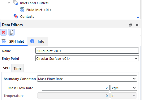
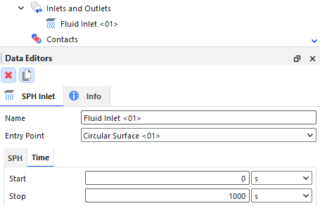
Table 3.3: Fluid Inlet parameter options
| Setting | Description | Range |
|---|---|---|
| Name |
Enables you to specify a unique identifier for the fluid inlet. | 99 character limit |
| Entry Point | The surface inlet from which the fluid is released during the simulation. Note: Only one Inlet can be set per Entry Point. | Any Planar Surface |
| SPH | ||
| Mass Flow Rate | The mass flow rate forthe Fluid elements that you want released from this Entry Point | Values above but not equal to 0 kg/s Note: The one exception to this rule is if you want to change the active Inlets after you save a copy of a partially processed pimulation for pestart purposes. |
| Temperature | When Thermal Model is enabled this is the temperature that all particles in the Particleset will have when released from this Entry point. | Values above but not equal to 0 K (zero Kelvin) |
| Time sub-tab | ||
| Start | The time you want fluid elements to begin releasing from the Entry Point. | Positive values Note: Check the Status panel to ensure that any variables or mathematical functions you might use results in valid values. |
| Stop | The time you want fluid elements to stop releasing from the Entry Point. Note: If you choose to use parametric expressions in this field, know that only the resulting value and not the variables and/or mathematical functions you enter will be retained in any project copies you save for restart purposes. | Positive values Note: Check the Status panel to ensure that any variables or mathematical functions you might use results in valid values. |
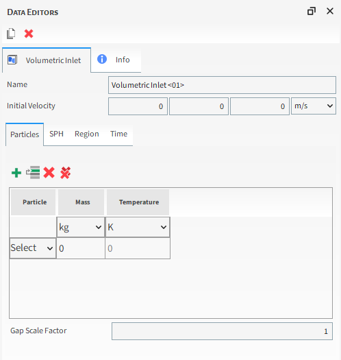
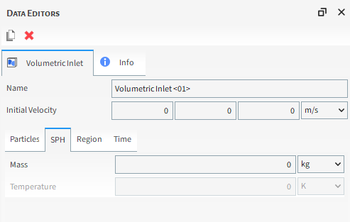
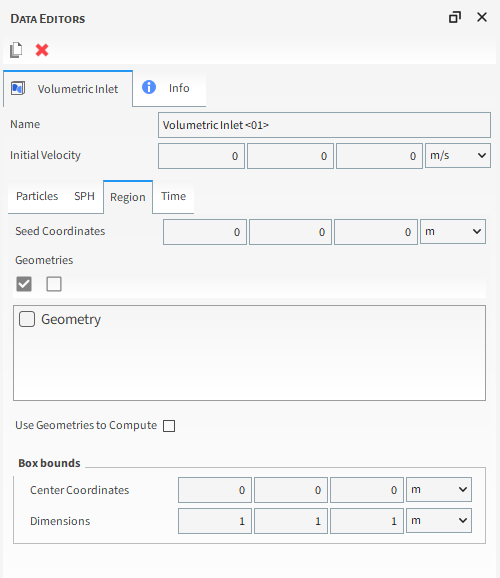
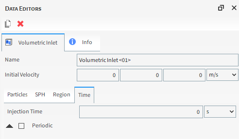
Table 4: Volumetric Inlet parameter options
|
Setting |
Description |
Range |
|---|---|---|
|
Name |
Enables you to specify a unique identifier for the inlet. |
99 character limit |
| Initial Velocity | Enables you to set a vector of initial velocities in the x, y and z-axis
for both DEM particles and SPH elements. Important: The initial velocities vector is the same for all DEM particles and all SPH elements defined on the same volumetric inlet. Note: The initial velocities vector cannot be changed for resume or restart simulations. | Any values |
|
Particles sub-tab | ||
|
Particle |
The Particle set that you want to enter into simulation by building around the Seed Coordinate, which is itself specified on the Region sub-tab. |
Any Particle set specified in the simulation |
|
Mass |
The target mass of particles within the set that you want built around the Seed Coordinate, which is itself specified on the Region sub-tab. Tip: To avoid entering a value that is too large to fully simulate, ensure that you are entering a Mass value appropriate for the Particle set and Box volume you specify on the Region sub-tab. |
Values above but not equal to 0 kg |
|
Temperature |
When Thermal Model is enabled (see also About Physics Parameters), this is the temperature that all particles in the Particle set will have when injected from this inlet method. |
Values above but not equal to 0 K (zero Kelvin) |
|
SPH sub-tab | ||
|
Mass |
The target mass of fluid within the set that you want built around the Seed Coordinate, which is itself specified on the Region sub-tab. Tip: To avoid entering a value that is too large to fully simulate, ensure that you are entering a Mass value appropriate for the box volume you specify on the Region sub-tab. |
Values above but not equal to 0 kg |
|
Temperature |
When Thermal Model is enabled (see also About Physics Parameters), this is the temperature that the fluid elements will have when injected from this inlet method. |
Values above but not equal to 0 K (zero Kelvin) |
|
Region sub-tab | ||
|
Seed Coordinates |
The X, Y, and Z coordinate location of the point ("Seed") around which the particle layers will be built. Tip: To avoid particle generation issues, ensure that you locate your Seed Coordinate away from the boundaries of your simulation geometries. |
No limit but the location must be within the limits of the Volumetric Inlet Box bounds |
|
Gap Scale Factor |
Determines how closely particles are positioned to each other (i.e., how much of a "gap" there is between them) during injection. Specifically:
|
1 or greater |
|
Geometries |
Lists the imported geometry components within the simulation by which you are able to constrain your Volumetric Inlet. Specifically:
|
Turns off or on |
|
Use Geometries to Compute |
When one or more geometry components are selected from the Geometries list, selecting this option enables Rocky to automatically define the Box bounds based upon the limits of the selected geometries. When this option is cleared, Rocky will use the Box bounds you define. |
Turns off or on |
|
Box bounds Center Coordinates |
When the Use Geometries to Compute checkbox is cleared, this defines the X, Y, and Z coordinate location of the boundary box's center point. (The bounds of this box is what will constrain your Volumetric Inlet.) |
No limit |
|
Box bounds Dimensions |
When the Use Geometries to Compute checkbox is cleared, this defines the X, Y, and Z dimensions of the box that will constrain your Volumetric Inlet. |
No limit |
| Time sub-tab | ||
| Injection Time | The simulation time at which you set the volumetric injection to occur. | Positive values |
| Periodic | Enables periodic volumetric injection of Particles and/or Fluid into the simulation. | Turns on or off |
| Period Time | The period at which you set the volumetric injection to occur. | Positive values |
| Stop Time | The simulation time at which you set the periodic injection to stop. | Positive values |
|
Modules sub-tab | ||
|
Particle |
For each row, lists the Particle set that is defined on the Particles sub-tab. |
Automatically provided |
|
(Varies) |
These settings are specific to only certain external Module and are therefore not documented in the Rocky User Manual. Refer to the Module's documentation (if provided) for more information. (See also Rocky Simulation Entities that can be Affected by Modules). |
(Varies) |
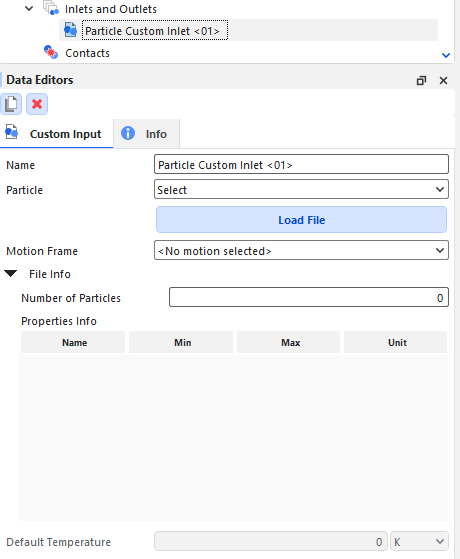
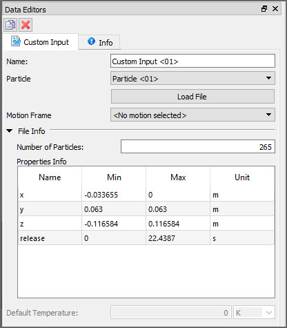 Figure 20: Particle Custom Inlet, Data
Editors panel when a multi-element (flexible and/or discrete-breakable) Fiber with
frozen elements is defined
Figure 20: Particle Custom Inlet, Data
Editors panel when a multi-element (flexible and/or discrete-breakable) Fiber with
frozen elements is defined
Note: The Overlap Check for Particle Custom Inlet injection only works when the particle is released at t>0s. If the particle is released at t=0s, this overlap check is not performed.
Table 5: Particle Custom Inlet parameter options
|
Setting |
Description |
Range |
|---|---|---|
|
Name |
Enables you to specify a unique identifier for the particle inlet. |
99 character limit |
|
Particle |
Enables you to select which of the available particle sets to apply to the Particle Custom Inlet. |
Automatically determined |
|
Motion Frame |
When a multi-element (flexible and/or breakable) Custom Fiber with frozen elements defined is selected for the Particle, this defines which Motion Frame you want assigned to the frozen elements of the injected fibers. |
Automatically determined |
|
Number of Particles |
Lists the total amount of particles that will be released based upon this inlet into the simulation. This number is based upon the rows defined in the imported Particle Custom Inlet file. |
Display only |
|
Properties Info |
Displays a table of summarized details based upon the Particle Custom Inlet file that was imported. This data includes the field Name, which corresponds to the column header used within the file; the Min and Max values, which together summarize the range of values being used within the particles defined; and the Unit, which displays the hard-coded unit of measurement always used when defining that particular field type. |
Display only |
|
Default Temperature |
When the Thermal Model is enabled (see also About Physics Parameters) and no temperature values were defined in the imported Particle Custom Inlet file, this is the temperature that all particles in the Particle set will have at the time of release. |
Values above but not equal to 0 K (zero Kelvin) |
|
Other "Modules" Settings | ||
|
(Varies) |
These settings are specific to only certain external Module and are therefore not documented in the Rocky User Manual. Refer to the Module's documentation (if provided) for more information. (See also Rocky Simulation Entities that can be Affected by Modules). |
(Varies) |
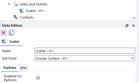
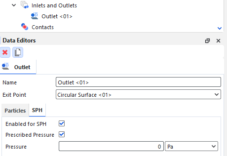
Table 6: Outlet parameter options
|
Setting |
Description |
Range |
|---|---|---|
|
Name |
Enables you to specify a unique identifier for the outlet. |
99 character limit |
|
Exit Point |
The surface that will act as an exit point for both, fluid and particles, during the simulation. |
Any Planar Surface |
|
Particles sub-tab | ||
|
Enabled for Particles |
Specifies if the outlet will act as an Exit Point for Particles. |
Turns off or on |
|
SPH sub-tab | ||
|
Enabled for SPH |
Specifies if the outlet will act as an Exit Point for Fluid. |
Turns off or on |
|
Prescribed Pressure |
Specifies if the outlet will use a Prescribed Pressure as a boundary condition. |
Turns off or on |
|
Pressure |
Defines the pressure that will be applied to the Prescribed Pressure boundary condition. |
Any Value |
What would you like to do?
From the Data panel, click Inlets and Outlets, and the from the Data Editors panel, click the Create Particle Inlet button. A new Particle Inlet component appears under Inlets and Outlets in the Data panel. Tip:You may also access this functionality from the right-click menu on the Data panel.
From the Data panel, click the Particle Inlet component you just added and then from the Data Editors panel, on the main Particle Inlet tab, enter the Name and set the Entry Point you want.
From the Particles sub-tab, do all of the following:
Click the Add button. A new row appears at the bottom of the table.
Under Particle, choose the Particle set that you want, and then specify the Mass Flow Rate and Temperature (if applicable) you want associated with that Particle set.
Repeat step 3 for each Particle set that you want entering the simulation from the Entry Point specified.
If desired, select the check box to allow for fluid elements inlet alongside the DEM particles and define the Temperature (if aplicable).
From the Time sub-tab, define what you want for Start and Stop times.
If desired, from the Entry sub-tab, define the Velocities parameters you want. Optionally, you can also define the Periodic injection settings you want.
If you have enabled a Module that has unique Input properties (see also About Modules Parameters), select the Modules sub-tab, and then for each Particle row specified, enter the value you want for the module-specific parameters provided.
Tips:
To insert a new row beneath the selected row, click the Insert button.
To remove the selected row, click the Remove button.
To remove all rows in the table, click the Remove All button.
To see an estimate of the number of particles that might be released from a Particle Inlet during the simulation, view the Info tab.
See Also:
From the Data panel, click Inlets and Outlets, and the from the Data Editors panel, click the Create Fluid Inlet button. A new Fluid Inlet component appears under Inlets and Outlets in the Data panel. Tip:You may also access this functionality from the right-click menu on the Data panel.
From the Data panel, click the Fluid Inlet component you just added and then from the Data Editors panel, on the main Fluid Inlet tab, enter the Name and set the Entry Point you want.
From the SPH sub-tab, do all of the following:
Set the Mass Flow Rate at the inlet.
If applicable, specify the fluid Temperature at the inlet.
From the Time sub-tab, define what you want for Start and Stop times.
See Also:
From the Data panel, click Inlets and Outlets, and the from the Data Editors panel, click the Create Volumetric Inlet button. A new Volumetric Inlet component appears under Inlets and Outlets in the Data panel. Tip:You may also access this functionality from the right-click menu on the Data panel.
From the Data panel, click the Volumetric Inlet component you just added and then from the Data Editors panel, on the main Volumetric Inlet tab, enter the Name you want.
To add Particles: From the Particles sub-tab, do the following:
Click the Add button. A new row appears at the bottom of the table.
Under Particle, choose the Particle set that you want, and then specify the Mass and Temperature (if applicable) you want associated with that Particle set.
Repeat steps 3a-3b for each Particle set that you want entering the simulation from the fill Region you will define.
To add Fluid: From the SPH sub-tab, do the following:
Set the total fluid Mass.|br|
If applicable, specify the fluid Temperature.
From the Region sub-tab, do the following:
Next to Seed Coordinates, enter the X, Y, and Z coordinate location of the spherical point around which your Volumetric Inlet layers will be built. Important: This must be located within your Box bounds. Tip:Avoid locating this directly on the boundaries of your simulation geometries.
If you want there to be some space between your particles when they are injected, enter a value above 1 for Gap Scale Factor. Otherwise, leave this setting as 1 to have particles injected closely together.
Do one of the following:
To have Rocky automatically calculate your Box bounds based upon one or more imported geometries in your simulation, select the geometries you want from the Geometries list, and then select the Use Geometries to Compute checkbox.
To define your own box bounds but still have your Volumetric Inlet constrained to one or more geometry components, select the geometries you want from the Geometries list, and then define the Center Coordinates and Dimensions of your Box bounds.
To define your own Box bounds and have your Volumetric Inlet ignore any geometries within the bounds you define, keep both the Geometries and the Use Geometries to Compute checkboxes cleared, and then define the Center Coordinates and Dimensions of your Box bounds.
If you have enabled a Module that has unique Input properties (see also About Modules Parameters), select the Modules sub-tab, and then for each Particle row specified, enter the value you want for the module-specific parameters provided.
Tips:
For the Region tab:
To visualize the Box bounds and Seed location of your Volumetric Inlet input, select or create a 3D View window and then from the Data panel, select the Volumetric Inlet entity you want to see. (See also View Geometries, Particles, Points, and Fluids in 3D.)
In the 3D View window, you can also move and resize the fill area by clicking and dragging the handles (colored dots) representing the center, and the local X, Y, and Z locations respectively. (See also Use Colored Directional Handles.) Note: You still must move the Seed location by using the Seed Coordinates.
For the Particles tab:
To insert a new row beneath the selected row, click the Insert button.
To remove the selected row, click the Remove button.
To remove all rows in the table, click the Remove All button.
To see an estimate of the number of particles that might be released from a Particle Input during the simulation, view the Info tab. Notes:
This estimate assumes there are no boundary limits to consider and that the Gap Scale Factor is equal to 1.
Ensure that the estimate includes enough particles; Volumetric Inlets require a minimum of 3 particles in order to create the "Seed". (See also Particle and Input Limitations.)
See Also:
In a spreadsheet program or text editor, use the formatting requirements (see also About Adding and Editing Particle Inlets and Outlets) to define the fields and values you want for each particle you want injected, and then save the file as one of the supported CSV or Excel/ODF file formats (see also File Types and Folders in Rocky) ensuring that the file is saved so that the values are separated by commas (sometimes called comma delimited or Comma Separated Value files). Important: If you intend to use frozen Fibers, you must ensure that all release times are either be defined as 0 (zero) or the release field itself is omitted from the Custom Input definition file.
From the Data panel, click Inlets and Outlets, and the from the Data Editors panel, click the Create Particle Custom Input button. A new Custom Input component appears under Inlets and Outlets in the Data panel. Tip:You may also access this functionality from the right-click menu on the Data panel.
From the Data panel, click the Custom Input component you just added and then from the Data Editors panel, on the main Particle Custom Input tab, enter the Name you want, and then select the Particle set you want to use.
Click the Load File button.
From the Select file to import dialog, navigate to and select the definition file you saved in step 1, and then click Open. The table and fields under File Info on the Data Editors panel will display summary information from the file you imported.
If for the Particle parameter, you chose a multi-element (flexible and/or discrete-breakable) Custom Fiber particle set that was defined using frozen Segments (also known as a Frozen Fiber shape; see also About Defining and Importing Custom Particle Shapes), and you want those frozen Segments to have motion assigned, select the motion you want applied from the Motion Frame list. Note: Unlike with custom geometries, particles assigned Motion Frames will not be visible in the Motion Preview window. (See also About Motion Preview Windows.)
If you have enabled the Thermal Model for your simulation (see also About Physics Parameters) and the file you imported did not include a temperature column, you must also define what Default Temperature you want your particle set to have when released.
If you have enabled a module for your simulation that requires a Particle Input parameter that was not defined in the custom injection file you imported, you must also define that parameter in the field provided on the Particle Custom Input tab.
See Also:
From the Data panel, click Inlets and Outlets, and the from the Data Editors panel, click the Create Outlet button. A new Outlet component appears under Inlets and Outlets in the Data panel. Tip:You may also access this functionality from the right-click menu on the Data panel.
From the Data panel, click the Outlet component you just added and then from the Data Editors panel, on the main Outlet tab, enter the Name and set the Exit Point you want.
From the Particles sub-tab, clear the Enabled for Particles if you do not want particles to be able to leave the simulation through this outlet. By default the checkbox is checked.
From the SPH sub-tab, do all of the following: a. Clear the Enabled for Particles if you do not want fluid to be able to leave the simulation through this outlet. By default the checkbox is checked. b. Select if you want to use a Prescribed Pressure boundary condition at the outlet. c. If the Prescribed Pressure option was selected, define the pressure that you want prescribed at this outlet.
See Also:
From the Data panel, click the Inlet or Outlet you want to edit, and then from the Data Editors panel, modify the settings as desired.
See Also:
From the Data panel, click the Inlet or Outlet you want to remove, and then from the Data Editors panel, click the Remove button.
See Also:
Whenever a particle collides with another particle or boundary during a simulation, Rocky detects and calculates those interactions as one (or more) separate, individual contacts.
Rocky always calculates and makes use of both frictional and adhesive (if available) contacts data during simulation processing, but allows you to turn off the long-term collection of this data to reduce your files size.
You are able to post-process and visualize the contacts data that you choose to collect.
The collection of this data, as well as the post-processing and visualization, is done through a Contacts entity that appears on the Data panel under Study.
Important: Turning on Contacts data collection prior to processing is a requirement for post-processing and/or visualization of the data later.
What would you like to do?
See Also:
A contact in Rocky refers to a specific location on a boundary or particle that has experienced a collision with another particle during the simulation.
In addition to frictional contacts, which are the default type of contact calculated in Rocky, you can also collect adhesive contacts in this version. Adhesive contacts are present only if an Adhesive Force model is enabled in the simulation. (See also About Physics Parameters.)
Rocky always calculates both frictional and adhesive contacts and makes use of that data during simulations. But you can also choose whether or not to keep one or both types of data after Rocky has used it. If you do choose to collect it, you can analyze and visualize that data (Figure 1) after processing, just like other kinds of data in Rocky. However, you must choose to collect it before processing a simulation.
Figure 3.206: Frictional contacts data being visualized with particles (top) and without particles (bottom)
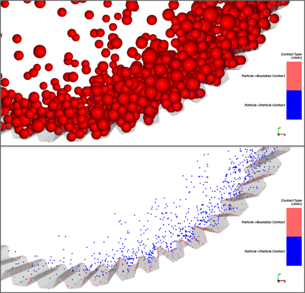
The Collect Contacts Data checkbox, which is located on the Data panel's Contacts entity, is what determines whether or not the frictional-contact-related data required to calculate particle and boundary movement is saved for each output. The sub-checkbox Include Adhesive Contacts is what determines whether the adhesive-contact-related data is also saved. Note: You cannot save only adhesive contacts data. To save adhesive contacts data, you must also save frictional contacts data.
If you choose to enable one or both checkboxes prior to processing your simulation, your simulation file size will be larger but you will gain both of the following benefits:
You will be able to analyze and visualize contacts data after processing.
Resuming a Stopped simulation will be quicker as the contact data will be readily available.
When these checkboxes are cleared (default state), your simulation file size will be smaller but you will not be able to analyze nor visualize contacts data after processing and Resuming a Stopped simulation will take more time as the contact data for the in-process output time will need to be recalculated before Processing is Resumed.
Tip: View walk-through examples of collecting frictional contacts data in the following Workshops:
If you have chosen to collect contacts data prior to processing, you will be able to post-process this data by using several new properties and user processes. See the sections below for more details.
A new property for Particles called Stress Tensor is available, plus several new stress-related properties for Eulerian Statistics.
See also the definitions in the Particles Properties (Simulation-Wide) and the Eulerian Statistics Properties sections of the About Properties topic.
A new category of properties are available for the Contacts entity itself, enabling you to analyze coordinate locations, forces, and more for each contact.
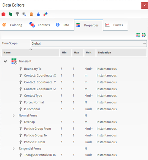
See also the Contacts Properties section of the About Properties topic.
This functionality enables you to visualize 1D line segments connecting the centers of each particle that are interacting in a contact (Figure 3).
Figure 3.208: Particle-to-particle contact data visualized as line segments being shown with particles (top) and without particles (bottom)
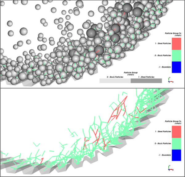
This is accomplished by enabling the Edges option and then selecting the contact-related property you want to visualize.
Notes:
Only particle-to-particle data can be visualized in a contact network; particle-to-boundary connections can not be visualized in this way—even if they are shown on the color scale. (See also About Color Scales.)
Contact properties that can be visualized in a network are defined in the About Properties topic.
Information about how to use the Edges option can be found in the About Using the Coloring Tab to Change a 3D View topic.
In addition to the new properties, there are two User Processes specifically designed for use with Contacts:
Particle to Contact: This is designed to filter out which contacts are happening to a particular sub-set of particles. For example, you can:
Create a filter process of a particular particle group and then use the Particle to Contact User Process to analyze normal forces or overlaps from collisions involving the desired particle shape.
Create a filter process of particles within a given velocity range and then use the Particle to Contact User Process to analyze normal forces or overlaps from collisions involving them.
This User Process is created from the main Particles entity or another User Process based upon it. Even though you create this User Process from Particles, its parent entity is Contacts. This means that after applying this User Process, you are able to further analyze the contacts by Contacts Properties.
Contact to Particle: This is designed to filter out which particles are experiencing a particular sub-set of contacts. For example, you can:
Create a filter process of contacts affecting a particular boundary and then use the Contact to Particle User Process to analyze the particle properties-size distribution or size groups, for example-of these filtered contacts only.
Create a filter process of contacts with overlaps greater than a certain value, and then use the Contact to Particle User Process to analyze the PSD of those filtered particles. This can help you better understand why high overlaps are occurring with certain particles.
This User Process is created from the main Contacts entity or another User Process based upon it. Even though you create this User Process from Contacts, its parent entity is Particles. This means that after applying this User Process, you are able to further analyze the particles by Particles Properties.
Important: Even though both the Contact to Particle and the Particle to Contact User Processes will always be available, there will be no Contacts data to analyze unless you turn on the collection of Contacts data prior to processing your simulation. (See also Turn On Contacts Data Collection.)
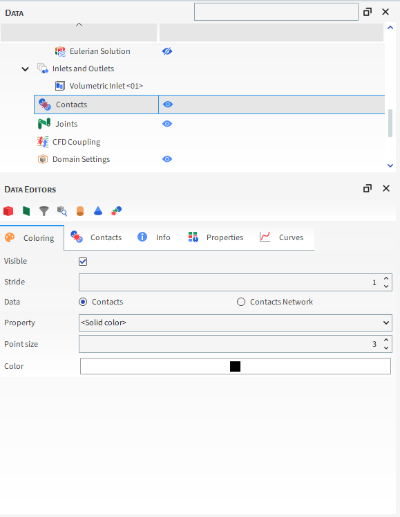

Table 3.4: Contacts Parameters - Coloring
|
Setting |
Description |
Range |
|---|---|---|
|
Visible |
When enabled, shows the selected entity in the active view window. |
Turns on or off. |
|
Stride |
One out of this number of data points will be shown when displaying Contacts. The lower the number, the more data points will be displayed. |
Whole numbers 1 or greater. |
|
Data |
Contacts: Enables the selected contacts to be colored in the 3D View. Contacts Network: Enables the selected connections between contacts to be colored in the 3D View. |
Options limited by the selected Data. |
|
Property |
Provide properties and other color options that apply to the display Data type within which the list is contained.
|
<Solid color>; List of properties automatically generated from the Properties tab. |
|
Point size |
When Contacts is selected, this changes the size of the dots used to draw the Contacts. |
Positive Values. |
|
Width |
When Contacts Network is selected, this changes the thickness of Positive values the lines used to draw the borders. |
Positive Values. |
|
Color |
When Contacts and Contacts Network are selected and the Property is <Solid Color>, this enables the selected display Data type to be colored in the one solid color chosen. |
Options limited by the selected Color. |
Use the figure and table below to help you understand the various Contacts parameters you can set for a simulation project.
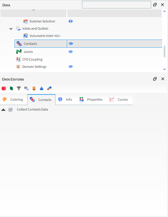
Table 1: Contacts parameter options
Setting | Description | Range |
|---|---|---|
Collect Contacts Data | Determines whether or not the frictional-contacts- related data required to calculate particle and boundary movement is saved for each Output Time. When enabled, simulation file size will be larger but you will be able to visualize and analyze Contacts data later and Resuming a Stopped simulation will be quicker as the contact data will be readily available. When cleared, simulation file size will be smaller but you will not be able to visualize nor analyze Contacts data later and Resuming a Stopped simulation will take more time as the contact data for the in-process output will need to be recalculated before Processing is Resumed. See also Resume Processing a Stopped Simulation. | Turns on or off |
Include Adhesive Contacts | When an Adhesive Force is enabled, Rocky also saves for each Output Time the adhesive-contacts- related data required to calculate particle and boundary movement. | Turns on or off |
What would you like to do?
Learn more Analyzing a Simulation
Learn more about Analyzing Contacts from a Sub-Set of Particles
Learn more about Analyzing Particles from a Sub-Set of Contacts
See Also:
Set up your simulation as you normally would. (See also Setting Up a Simulation.)
Prior to processing your simulation, do all of the following:
From the Data panel, click Contacts.
From the Data Editors panel, do one or both of the following:
Enable the Collect Contacts Data checkbox, which will save frictional contacts data.
(Optional) If you have enabled an Adhesive Force model, enable the Include Adhesive Contacts checkbox, which will also save adhesive contacts data. (See also About Physics Parameters.)
Process your simulation as you normally would. (See also Processing a Simulation.) The contacts data you chose to collect is available for post-processing.
See Also:
In this version of Rocky, Contacts Data collection is turned off by default. However, if you have already turned on Contacts Data collection but now want to turn it off, you can use the following procedure.
Prior to processing your simulation, do all of the following:
From the Data panel, click Contacts.
From the Data Editors panel, ensure that both the Include Adhesive Contacts and the Collect Contacts Data checkboxes are cleared (unchecked).
Process your simulation as you normally would. (See also Processing a Simulation.) The simulation file sizes are smaller and there are no Contacts data available for post-processing.
See Also:
In Rocky, there are several different methods for simulating the interaction between particles and the surrounding fluids (air, water, dust, etc.), known more commonly as Computational Fluid Dynamics (CFD). The CFD Coupling categories and methods available in Rocky are described below:
1-Way | Particle → Fluid: In this method, particle flow affects the fluid flow but the fluid flow does not, in turn, affect the particles. In this, it is considered a one-way calculation and includes only the LBM option, which simulates how particles change the flow of fluids that are calculated using the Lattice Boltzmann Method (LBM).
1-Way | Fluid → Particle: In these methods, the fluid flow affects the particle flow but the particle flow does not, in turn, affect the fluid flow. These are also considered one-way calculations and include the following two methods:
The Constant method, which simulates how a constant fluid flow changes the flow of particles in Rocky.
The Fluent method, which simulates how the steady state or transient fluid flow calculated in Ansys Fluent changes the flow of the particles with which they come into contact in Rocky.
2-Way | Fluid [left-right arrow] Particle: In these methods, the fluid flow affects the particle flow and vice versa, resulting in a truly two-way coupled simulation. This version of Rocky includes the following methods:
The Fluent method, which considered an unresolved method and is appropriate for most 2-Way coupling cases.
The Fluent Semi-Resolved method, which is a special 2-Way coupling method most appropriate for a few, very large (when compared to the cell size of the Fluent mesh) particles interacting with a dynamic fluid whose accurate behavior requires a very refined Fluent mesh. It should be used in cases where the resolution of the fluid flow around the particles is critical to capturing the behavior of the particles, and relying on standard correlations for fluid forces based on the centroid fluid velocity and velocity gradients isn't sufficient.
You may choose only one CFD Coupling method per simulation project file. However, for most of these methods, you can choose how the data is visualized in the Coloring tab. (See also Create and Modify a 3D View.)
See further details in the sections below.
This method is useful in cases where you have a known, unchanging fluid flow and want to understand how it impacts the flow of particles without having to use a separate CFD program. You can set a constant value for density, velocity, viscosity (and thermal properties if thermal is being solved), and Rocky will use those values to simulate the fluid flow.
For example, with this method you can simulate the relative buoyancy of a dense and light material through water (Figure 2), or simulate the relative speed of a stretched and compact shape through air.
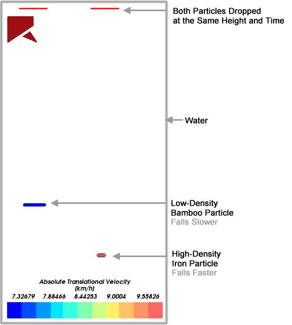
With this method, the particle flow does not affect the fluid flow.
This method is accomplished by enabling Rocky to calculate how particle flow and the boundaries that contain those particles affects the air that comes into contact with them. This method uses the Lattice Boltzmann Method (LBM) for its calculations and is useful for simulating how much dust a transfer chute design would generate, for example. In this method, the air flow does not affect the movement of the particles; only the particles and the boundaries affect the air flow. (See Figure 1 for an example.)

This method is accomplished by a one-way coupling with Ansys Fluent-using either steady state or transient data.
In this method, a CFD simulation done within Fluent calculates the velocity and pressure fields generated by the fluid as it flows through the equipment being studied. Once that Fluent case is complete, you can choose one of two data export methods within Fluent:
Export a single file of the fluid data at steady state.
Record and then export a set of transient fluid data.
After you export this data out of Fluent, you import it into Rocky. During the simulation, Rocky will then calculate how the fluid flow would affect the particle flow.
This method is particularly useful for simulating the effect of water on the movement of particles through a pipe, for example. Or, for simulating the transport of particles with different densities by water in a slurry-like flow. In the 1-Way Fluent method, the particles do not affect the fluid flow; the fluid flow affects the movement of the particles. (See Figure 3 for an example.)
While the fluid data must still come from Fluent, with the 1-Way Fluent method it is not necessary to have both Rocky and Fluent installed on the same machine.
Figure 3.214: 1-Way Fluent with steady state fluid data showing how particles interact with the fluid-like vectors
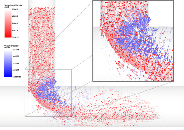
This unresolved method is particularly useful for simulating complex phenomena such as pneumatic conveying, granular drying, slurry flow inside grinding mills, or even chemical reactions between particles and fluids. In the 2-Way Fluent method, the particles are part of the fluid flow and will affect it in a two-way interaction: particles are affected by other particles and the fluid around it while the fluid flow is also affected by the particle pressure. (See Figure 4 for an example.)
In this method, correlations for fluid forces acting on particles (such as drag, lift, and virtual mass) are calculated based on the fluid quantities (such as velocity and velocity gradient) of the cell where the centroid of the particle is located. This flow approximation means that your mesh can be larger than with the 2-Way Fluent Semi-Resolved method.
Unlike the 1-Way Fluent Method, for the 2-Way Fluent method to work, both Fluent and Rocky must be installed on the same host machine.
This semi-resolved method is useful in cases where the resolution of the fluid flow around the particles is critical to capturing the behavior of the particles, and relying on standard correlations for fluid forces based on the centroid fluid velocity and velocity gradients-as done in the standard 2-Way Fluent method-isn't sufficient. Rather than solving correlations based upon the centroid velocities, fluid forces are integrated at the particle's surface in the semi-resolved method, which requires a very fine mesh around the particle in order to work properly.
This method therefore requires a certain number of cells to define the particle surface, which means a particle-grid size ratio greater than 10. The finer the mesh resolution, the more accurate the results (but also, the more computationally expensive the simulation).
This method works with both single-phase and multiphase flows and accepts spheres, shells (both rigid and flexible), and custom solid shapes (rigid only).
Like the standard 2-Way Fluent method, the 2-Way Fluent Semi-Resolved method requires that both Fluent and Rocky be installed on the same host machine.
What would you like to do?
See Also:
The 1-Way Constant CFD Coupling method simulates how a constant fluid flow changes the flow of particles in Rocky without the need for a separate CFD Program.
What would you like to do?
See Also:
The 1-Way Constant CFD Coupling method uses the known, unchanging fluid values you provide to simulate a constant fluid flow in Rocky, without the need for a separate CFD Program. Because the fluid flow stays constant throughout the whole simulation, it is somewhat more limiting when compared to the 1-Way Fluent, but can still be quite useful in certain situations. For example, when simulating the fluid's effect on particles as objects are dropped through water or air.
The 1-Way Constant method is also compatible with Thermal Modeling, so you can also simulate how the temperature of the fluid affects the particles that come into contact with it.
When combined with Coarse Grain models, only drag forces are considered. This means that other non-drag fluid force models, such as virtual mass and lift, are incompatible with Coarse Grain modeling. (See also About Physics Parameters.)
In addition, Shell and Solid particles composed of Multiple Elements (also known as meshed or flexible particles) are incompatible with 1-Way Constant coupling. The only flexible particle shapes compatible with this feature are Fibers. (See also About Adding and Editing Particle Sets.)
For a full list of limitations, refer to the Ansys and CFD Coupling Limitations topic.
Use the figures and table below to understand the various parameters you can set for 1-Way Constant.
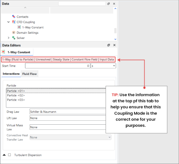
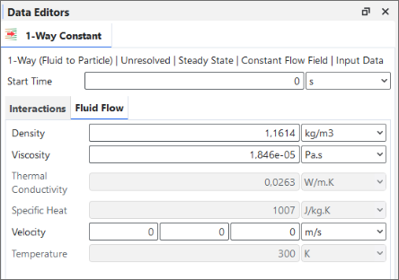
Table 1: 1-Way Constant Settings (all tabs)
Setting | Description | Range |
|---|---|---|
Start Time | The time during the simulation when you want to start taking fluid flow into account. | Positive values |
Interactions tab | ||
Particle | Permits correlations- such as drag, lift, virtual mass, and convective heat transfer laws (if applicable)- to be defined per Particle set. You accomplish this by selecting (or multi-selecting) from a list of previously defined Particle sets, and then defining the applicable CFD Laws for only the selected set (or sets). Important: Even though they will still be listed here, neither flexible Shell nor flexible Solid particle shapes are supported in CFD Coupling approaches, including this one. (See also Ansys and CFD Coupling Limitations). | Automatically provided |
Drag Law | Correlation used by Rocky to calculate drag forces on particles (with the exception of Fiber and also Solid Sphero-Cylinder shapes-see note below):
Note: Unless stated otherwise, the above drag laws apply to any supported particle shapes (see also Ansys and CFD Coupling Limitations) except Fiber and also Solid Sphero-Cylinder shapes, which have their own modified drag law based on the work by Marheineke and Wegener that should always be used for those shapes. Tip: For more information about these laws, refer to the CFD Coupling Technical Manual. (From the Rocky Help menu, point to Manuals, and then click CFD Coupling Technical Manual.) | Schiller & Naumann; Haider & Levenspiel; Ganser; Dallavalle: Marheineke & Wegener; Morsi & Alexander Note: If you have an external Module that adds in an additional CFD law, you must use that law at least once in your simulation project if the Module is enabled. Refer to the Module's documentation (if provided) for more information. (See also Rocky Simulation Entities that can be Affected by Modules). |
Lift Law | Correlation used by Rocky to calculate the fluid-particle force transversal to the direction of the relative velocity. | None; Saffman; Mei Note: If you have an external Module that adds in an additional CFD law, you must use that law at least once in your simulation project if the Module is enabled. Refer to the Module's documentation (if provided) for more information. (See also Rocky Simulation Entities that can be Affected by Modules). |
Virtual Mass Law | Correlation used by Rocky to calculate the virtual mass coefficient. | None; Constant Note: If you have an external Module that adds in an additional CFD law, you must use that law at least once in your simulation project if the Module is enabled. Refer to the Module's documentation (if provided) for more information. (See also Rocky Simulation Entities that can be Affected by Modules). |
Convective Heat Transfer Law | When Thermal Model is enabled (see also About Physics Parameters) this correlation is used by Rocky to calculate the fluid-particle convective heat transfer coefficient. | None; Ranz & Marshall; Whitaker Note: If you have an external Module that adds in an additional CFD law, you must use that law at least once in your simulation project if the Module is enabled. Refer to the Module's documentation (if provided) for more information. (See also Rocky Simulation Entities that can be Affected by Modules). |
Morsi & Alexander Parameters Use Defined Constants | When Morsi & Alexander is selected for Drag Law, this enables you to determine how the model's three coefficients will be determined. Specifically:
| Turns on or off |
| When Use Defined Constants is enabled, this is the value you
want assigned to the | Any value |
| When Use Defined Constants is enabled, this is the value you
want assigned to the | Any value |
| When Use Defined Constants is enabled, this is the value you
want assigned to the | Any value |
Turbulent Dispersion | Determines whether or not the dispersion of particles due to turbulence will be accounted for. Specifically:
| Turns on or off |
Turbulent Kinetic Energy | When Turbulent Dispersion is enabled, this is the amount of (constant) turbulent kinetic energy that will be used when modeling particle dispersion due to turbulence. | Positive values |
Turbulent Dissipation Rate | When Turbulent Dispersion is enabled, this is the (constant) turbulent kinetic energy dissipation rate that will be used when modeling particle dispersion due to turbulence. | Positive values |
Buoyancy | Determines whether or not hydrostatic pressure, which is used for buoyancy calculations, is included for the fluid-particle interactions. Note: This setting applies to all fluid-particle interactions regardless of what is selected for Particle. | Turns on or off |
Fluid Flow tab | ||
Density | The constant density of the fluid. | Positive values |
Viscosity | The constant viscosity of the fluid. | Positive values |
Thermal Conductivity | When Thermal Model is enabled (see also About Physics Parameters) this is the constant thermal conductivity of the fluid. | Any value |
Specific Heat | When Thermal Model is enabled (see also About Physics Parameters) this is the constant specific heat value of the fluid. | Any value |
Velocity | The constant velocity vector of the fluid, the magnitude of which is made up of the x, y, and z components respectively. | Any value |
Temperature | When Thermal Model is enabled (see also About Physics Parameters) this is the constant temperature of the fluid. | Values above but not equal to 0 K (zero Kelvin) |


What would you like to do?
See Also:
If you want to model thermal properties in your simulation, ensure you enable the Thermal Model during the Set Simulation-Wide Parameters step. (See also Enable Thermal Modeling Calculations.)
From the Data panel, click CFD Coupling and then from the Data Editors panel, choose Constant (Fluid → Particle) from the Coupling Mode list. The 1-Way Constant component appears in the Data panel beneath CFD Coupling.
In the Data panel, click the new 1-Way Constant component.
From the Data Editors panel, on the 1-Way Constant tab, do the following:
Set the Start Time you want.
On the Interactions tab, do the following:
From the Particle list, select (or multi-select) the Particle set name(s) for which you want to define particle-fluid interactions, and then select the various CFD laws you want for the selected set(s).
Select what you want for Turbulent Dispersion and Buoyancy.
On the Fluid Flow tab, define the constant Density, Viscosity, Velocity, and other thermal-related values you want.
The fluid flow data will be calculated when you process the simulation. (See also Processing a Simulation.)
See Also:
This type of CFD Coupling uses the Lattice Boltzmann Method (LBM) to simulate how the density, viscosity, and size of the air flow cells is affected by the particle flow.
What would you like to do?
See Also:
This type of CFD Coupling uses the Lattice Boltzmann Method (LBM) to simulate how air and dust flow are affected by the flow of particles in the simulation. Because of this, air flow changes as the simulation progresses. You need no special files to conduct this kind of analysis but note that the extra calculations will slow down the simulation processing.
At any point, you can see how your 1-Way LBM simulation results look in a 3D View (see also Create and Modify a 3D View).
Tip: For a self-guided walk-through example of setting up and running a simulation using the Lattice Boltzmann (LBM) Air Flow Method, refer to Tutorial - Discharge Air Flow in the Rocky Tutorial Guide.
The 1-Way LBM CFD Coupling method is incompatible with Coarse Grain Modeling. (See also About Physics Parameters.)
It is also incompatible with Shell and Solid particles composed of Multiple Elements (also known as meshed or flexible particles). The only flexible particle shapes compatible with this feature are Fibers. (See also About Adding and Editing Particle Sets.)
For a full list of limitations, refer to the Ansys and CFD Coupling Limitations topic.
Use the figure and table below to understand the various parameters you can set for 1-Way LBM.

Table 1: 1-Way LBM Settings
Setting | Description | Range |
|---|---|---|
Use Air Flow | Enables Lattice Boltzmann Air Flow calculations to be included in the simulation. | Turns on or off |
Start When Particles Enter | Enables Lattice Boltzmann Air Flow calculations to start as soon as particles appear in the air flow limit box. | Turns on or off |
Air Density | The density of the air. | Positive values |
Air Kinematic Viscosity | The kinematic viscosity of the air. | Positive values |
Cell Size | The size of an air flow cell. | Positive values |
Interaction Scale | Determines the interaction between the particle and the air. | Positive values. (It is recommended that the default value of 0.25 is used.) |
Start Time | When Start When Particles Enter is cleared, this is the time that Lattice Boltzmann Air Flow calculations begin during the simulation. | Positive values |
Speed of Sound | The speed of sound, which is used to calculate air flow. | Positive values |
Boundary Conditions | ||
First Derivative | This order provides more stability to the calculations but less accuracy. Tip: For more information on how Rocky calculates boundary conditions, see the 2000 paper by Verberg and Ladd entitled, "Lattice-Boltzmann Model with Sub-Grid-Scale Boundary Conditions." | Turns off or on |
Second Derivative | This order provides more accuracy to the calculations but less stability. | Turns off or on |
Coordinate Limits | ||
X Min/Max | Distance away from zero on the X axis to place the nearest and farthest corner of the air flow limit box. | No limit |
Y Min/Max | Distance away from zero on the Y axis to place the nearest and farthest corners of the air flow limit box. | No limit |
Z Min/Max | Distance away from zero on the Z axis to place the nearest and farthest corners of the air flow limit box. | No limit |
What would you like to do?
See Also:
From the Data panel, click CFD Coupling.
From the Data Editors panel, choose LBM (Particle → Fluid) from the Coupling Mode list. The 1-Way LBM component appears in the Data panel beneath CFD Coupling.
In the Data panel, click the new 1-Way LBM component.
From the Data Editors panel, on the 1-Way LBM tab, ensure the Use Air Flow checkbox is enabled, and then modify the settings as you want. The LBM air flow data will be calculated when you process the simulation. (See also Processing a Simulation.)
See Also:
From the Data panel, under CFD Coupling, click LBM (Particle → Fluid).
From the Data Editors panel, on the 1-Way LBM tab, modify the settings as you want.
See Also:
From the Data panel, under CFD Coupling, click LBM (Particle → Fluid).
From the Data Editors panel, on the 1-Way LBM tab, clear the Use Air Flow check box.
Tip: You can also remove 1-Way LBM from your set up completely by choosing No Coupling from the Coupling Mode list. (From the Data panel, click CFD Coupling and then from the Data Editors panel, make your selection on the CFD Coupling tab.)
See Also:
The 1-Way Fluent method provides an interface to generate a set of fluid flow data files in Ansys Fluent—-which can include air, water, and other fluids—-that you can then import into Rocky. In this version of Rocky, the fluid data you export can represent a steady state or transient flow.
This process can be conducted with Rocky and Fluent as standalone products, or through Ansys Workbench.
What would you like to do?
See Also:
The 1-Way Fluent Method is a CFD Coupling option that enables Rocky to receive fluid flow data from Ansys Fluent-at either a steady or transient state—and then calculate how the particles react to that flow.
It is called a 1-Way Coupling simulation because Rocky receives data only once from Fluent and sends nothing to Fluent in return.
Tip: You may also set up and process a 1-Way Fluent simulation within Ansys Workbench. To accomplish this with transient Fluent data, however, there are separate steps you must follow. (See also Set Up and Run a 1-Way Fluent Transient Project within Ansys Workbench.)
To make it possible to share the Fluent fluid flow data with Rocky, Rocky includes a special Ansys Fluent Coupling Support component. Installing this component enables a new Rocky Export menu option in Fluent (Figure 3.219: Rocky Export menu in Fluent) that allows the fluid data to be packaged into a unique "Fluent to Rocky" or F2R file, that later gets imported into Rocky as part of the 1-Way Fluent coupling process.
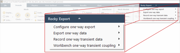
Table 1: Rocky Export menu in Fluent
|
Setting |
Description |
|---|---|
|
Configure one-way export | |
| Select Directory to Export | Choose the folder where the .cas and .dat files
will be saved. |
| Select Variables to Export | Select the variables to export, such as pressure, temperature, etc. |
| Select Wall Thermal Zones | Define the thermal zones to export. |
| Set Output Frequency | Define the frequency to export transient data. |
| Export one-way data | |
| Export current data to Rocky | Export the current static field data to Rocky. |
| Record one-way transient data | |
| Start one-way transient export | Start time recording transient one-way export data. |
| Stop one-way transient export | Stop time recording transient one-way export data. |
| Workbench one-way transient coupling | |
| Enable | Enable transient coupling with Workbench and Fluent (See also Set Up and Run a 1-Way Fluent Transient Project within Ansys Workbench.). |
| Disable | Disable transient coupling with Workbench and Fluent (See also Set Up and Run a 1-Way Fluent Transient Project within Ansys Workbench.). |
Important: Although 1-Way coupling does not require that Fluent be installed on the same Rocky machine running the coupled simulation, the machine exporting the fluid data out of Fluent must first have this Ansys Fluent Coupling Support component installed through the Rocky UI.
The Ansys Fluent Coupling Support component is included by default during your Rocky installation but if for some reason is not included or is in need of being updated, it can be installed later through the Rocky UI. (See also Install Ansys Coupling Components.)
1-Way coupled simulations also require that the initial CFD simulation be set up a certain way in Fluent to ensure that it works correctly when coupled with Rocky. These required settings are outlined in the accompanying procedure Use the 1-Way Fluent Method to Process Fluent and Rocky Simulations, and more detailed information about the Fluent settings can be found in the CFD Coupling Technical Manual manual (from the Rocky Help menu, point to Manuals and then click CFD Coupling Technical Manual.)
In Fluent, there are separate steps for exporting steady-state fluid data, or recording transient fluid data. Both processes result in a special F2R file that gets saved to the same folder at the initial Fluent CAS file (or alternate folder if you choose to define one). This is the file you will import into Rocky during the 1-Way Fluent coupling process.
If the Fluent case has geometry motions, this information will also be included in the F2R file. Rocky will automatically create new Motion Frames from the F2R file in this case. (You will still need to assign those motions to the geometries later.)
In addition to the F2R file, these other files are also exported out of Fluent:
One .dat file is saved for every timestep to specify the values of the specified flow field.
If the mesh position does not change between outputs, then one mesh.dat file is saved to specify the CFD mesh position. Otherwise, if the mesh position changes between outputs, additional mesh.dat files are saved for every timestep.
The geometry components used in the Fluent case file are exported to STL files. These STL files (or the CAS file itself) can be later imported into Rocky to ensure consistency between the two programs.
Important: For 1-Way transient cases especially, the quantity of the .dat and .mesh.dat files can add up quickly. Ensure that you have enough storage space designated for the exported files, and that you are recording only the portion of the fluid data that you require for your analysis. Starting the recording after some fluid results have been processed, and recording only one full revolution of your case are a few ways you can help limit your file size.
After importing the Fluent F2R file into Rocky, Rocky will then display (in a 3D View window) a node at all the cell centroids of the imported Fluent mesh. And will create new Motion Frames representing the geometry motions, if the original Fluent case had them.
You can then define what Laws you want applied to the imported fluid, and set a Start Time of when you want the fluid flow to be included in the coupled simulation. After the simulation is processed, Rocky will use this information to calculate how the particle flow will change because of the fluid forces.
For steady-state flows, the fluid remains constant after the Start Time is reached. For transient flows, the flow will be transient after the Start Time is reached until the end of the transient recording, and then the flow will remain constant from that point on. Tip:To achieve a steadier flow, you can offset the Start Time with negative numbers.
The influence of the fluid flow on the particle motion is achieved by adding up all the fluid forces acting on the particle, such as drag and pressure forces, as well as non-drag forces like virtual mass force, Basset force, lift force, Saffman and Magnum forces (due to particle rotation), among others. Depending on the flow conditions, most of these forces can be ignored.
A drag force exerted on a spherical particle is different from a drag force that acts on a shaped particle. In this 1-Way Fluent coupling, various drag correlations are available based on particle type (spherical or shaped).
Because the fluid flow calculations are already complete, there is no additional processing load for Rocky when choosing this option.
When setting up the initial CFD simulation in Fluent, you can also enable heat transfer calculations, so that particles will change their temperature because of the heat transfer with the fluid. In order to compute these values, Rocky will require some thermal properties from the fluid; in order to get those properties, the Thermal Model must also be enabled in Rocky before the coupled simulation is processed. (See also Enable Thermal Modeling Calculations.) In this way, convective heat transfer between particles and fluids can be simulated.
Note: In this version of Rocky, there are no restrictions on the type of Energy Equation you define in Fluent.
Tip: To see a walk-through example of coupling with the 1-Way Fluent using steady state data, including convective heat transfer, refer to the following Workshop: Tutorial - Windshifter in the Rocky Tutorial Guide.
A shadow boundary is an internal boundary without thickness. Due to the way Rocky optimizes the representation of the CFD domain in order to increase the simulation speed, in rare situations particles may be placed in a neighboring cell when the L-E mapping is performed. This is not a problem in the great majority of cases; however, when such a thing happens near a shadow boundary, there is a small chance that the particle is misplaced on the wrong side of the boundary. In order to avoid this chance occurrence, Rocky will prevent coupled simulations from processing if they have polygonal cells at shadow boundaries.
To get around this limitation, add a thickness to your shadow boundaries, or avoid using polyhedron meshes around them.
You can choose to visualize in a 3D View window the fluid flow data represented by Nodes and/or Vectors. This display, when combined with Particle visualization, can provide you a fuller visual confirmation of your 1-Way coupled simulation (Figure 2).
Figure 3.220: Example of a (steady state) 1-Way Fluent simulation showing static fluid flow vectors (in blue), and transient particle nodes + vectors (in red)
(See also About Using the Coloring Tab to Change a 3D View and About Properties.)
Shell and Solid particles composed of Multiple Elements (also known as meshed or flexible particles) are incompatible with 1-Way Fluent coupling. The only flexible particle shapes compatible with this feature are Fibers. (See also About Adding and Editing Particle Sets.)
In addition, Shell particles composed of Single Elements (also known as "rigid" particles) are also incompatible with 1-Way Fluent coupling.
Also, note that when combined with Coarse Grain models, only drag forces are considered. This means that other non-drag fluid force models, such as virtual mass and lift, are incompatible with Coarse Grain modeling. Tip:To see a walk-through example of 1-Way Fluent in use with Coarse Grain Modeling, refer to Tutorial - Mixing Tee in the Rocky Tutorial Guide.
For a full list of limitations, refer to the Ansys and CFD Coupling Limitations topic.
Refer to Figure 1 above, as well as Figures 3-4 and the table below to help you understand the Rocky Export options in Fluent.
Figure 3.221: The Additional Variables Selector dialog in Fluent (left). These become custom Properties in Rocky after F2R import (right).
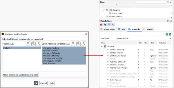
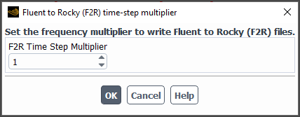
Table 1: Rocky Export menu options (in Fluent)
Menu Option | Description |
|---|---|
Configure one-way export | |
Select Directory to Export | Enables you to select where the exported F2R and related files will be saved. Note: If this is not defined, Fluent will automatically use the same folder as your Fluent case file. Important: Especially for transient files, the size and quantity of the exported files can add up quickly. Ensure that the directory you select has sufficient storage space. |
Select Variables to Export | Opens the Additional Variables Selector dialog (Figure 3, above), which enables you to define what Fluent variables—such as species, for example—you want included in the exported files. Each variable will come across as a separate Property that you can use in Rocky for post-processing (Figure 3, above). Because the variables can increase the size of the DAT files, limiting what variables you export to only what you require can help you control file size. |
Set Output Frequency | Opens the Fluent to Rocky (F2R) time-step multiplier dialog (Figure 4 above), which enables you to define how often you want the export process to save fluid files. For example, a F2R Time Step Multiplier of:
|
Export one-way data | |
Export current data to Rocky | For steady-state flows, exports fluid data at the currently selected Fluent Time Step. The resulting F2R file can then be imported into Rocky as part of the 1-Way Fluent coupling method. |
Record one-way transient data | |
Start one-way transient export | For transient flows, will begin the recording of fluid data at that point in the Fluent case processing. Tips:
|
Stop one-way transient export | For transient flows, will stop the recording of fluid data at that point in the Fluent case. The resulting F2R file can then be imported into Rocky as part of the 1-Way Fluent coupling method. Tip:It is recommended that you stop processing your Fluent case after the fluid data you want is calculated, and then select this option to stop recording your transient data. |
Workbench one-way transient coupling | |
Enable | For transient flows, enables you to set up and process the Rocky-Fluent coupled case through Ansys Workbench. (See also Set Up and Run a 1-Way Fluent Transient Project within Ansys Workbench). |
Disable | For transient flows, disables the ability to set up and process the Rocky-Fluent coupled case through Ansys Workbench. |
See the images and table below to help you understand the various properties you can set for the 1-Way Fluent method. For more information on this method, you may also refer to the CFD Coupling Technical Manual document included within the program. (From the Help menu, point to Manuals, and then click CFD Coupling Technical Manual.)
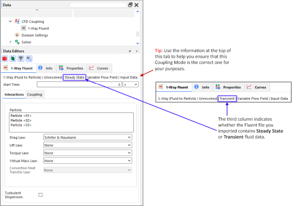 Figure 5 : CFD Coupling, 1-Way Fluent in the Data Editors
panel
Figure 5 : CFD Coupling, 1-Way Fluent in the Data Editors
panel
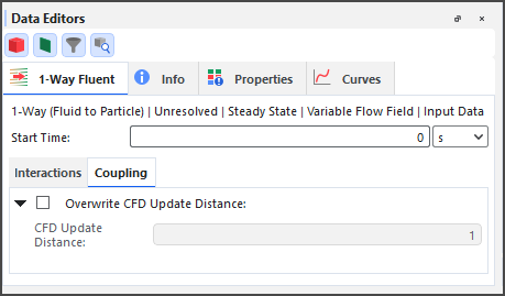 Figure 6 : CFD Coupling, 1-Way Fluent, Coupling Tab in the Data Editors
panel when Advanced Features are enabled
Figure 6 : CFD Coupling, 1-Way Fluent, Coupling Tab in the Data Editors
panel when Advanced Features are enabled
Table 2: 1-Way Fluent Settings (in Rocky, all tabs)
Setting | Description | Range |
|---|---|---|
Start Time | The time during the simulation when you want to start taking fluid flow into account. | Any value |
Interactions tab | ||
Particle | Permits correlations- such as drag, lift, torque, virtual mass, and convective heat transfer laws (if applicable)- to be defined per Particle set. You accomplish this by selecting (or multi-selecting) from a list of previously defined Particle sets, and then defining the applicable CFD Laws for only the selected set (or sets). Important: Even though they will still be listed here, neither flexible Shell nor flexible Solid particle shapes are supported in CFD Coupling approaches, including this one. (See also Ansys and CFD Coupling Limitations). | Automatically provided |
Drag Law | Correlation used by Rocky to calculate drag forces on particles (with the exception of Fibers and also Solid Sphero-Cylinder shapes-see note below):
Note: Unless stated otherwise, the above drag laws apply to any supported particle shapes (see also Ansys and CFD Coupling Limitations) except Fibers and also Solid Sphero-Cylinder shapes, which have their own modified drag law based on the work by Marheineke and Wegener that should always be used for those shapes. Tip: For more information about these laws, refer to the CFD Coupling Technical Manual. (From the Rocky Help menu, point to Manuals, and then click CFD Coupling Technical Manual.) | Schiller & Naumann; Haider & Levenspiel; Ganser; Dallavalle: Marheineke & Wegener; Morsi & Alexander Note: If you have an external Module that adds in an additional CFD law, you must use that law at least once in your simulation project if the Module is enabled. Refer to the Module's documentation (if provided) for more information. (See also Rocky Simulation Entities that can be Affected by Modules). |
Lift Law | Correlation used by Rocky to calculate the fluid-particle force transversal to the direction of the relative velocity. | None; Saffman; Mei Note: If you have an external Module that adds in an additional CFD law, you must use that law at least once in your simulation project if the Module is enabled. Refer to the Module's documentation (if provided) for more information. (See also Rocky Simulation Entities that can be Affected by Modules). |
Torque Law | Correlation used by Rocky to calculate the torque exerted by the fluid over the particle. | None; Dennis, Singh & Ingham Note: If you have an external Module that adds in an additional CFD law, you must use that law at least once in your simulation project if the Module is enabled. Refer to the Module's documentation (if provided) for more information. (See also Rocky Simulation Entities that can be Affected by Modules). |
Virtual Mass Law | Correlation used by Rocky to calculate the virtual mass coefficient. | None; Constant Note: If you have an external Module that adds in an additional CFD law, you must use that law at least once in your simulation project if the Module is enabled. Refer to the Module's documentation (if provided) for more information. (See also Rocky Simulation Entities that can be Affected by Modules). |
Convective Heat Transfer Law | When both Thermal Model is enabled (see also About Physics Parameters) and the Fluent exported results have thermal solution data, this correlation is used by Rocky to calculate the fluid-particle convective heat transfer coefficient. | None; Ranz & Marshall; Whitaker Note: If you have an external Module that adds in an additional CFD law, you must use that law at least once in your simulation project if the Module is enabled. Refer to the Module's documentation (if provided) for more information. (See also Rocky Simulation Entities that can be Affected by Modules). |
Turbulent Dispersion | When the imported .f2r file has a turbulent model that uses turbulence kinetic energy as one of its quantities, this allows those turbulent parameters to be used and modified in Rocky. Clearing this checkbox prevents the turbulent parameters from being used during the Rocky simulation. Tip: For more information about this parameter, refer to the CFD Coupling Technical Manual. (From the Rocky Help menu, point to Manuals, and then click CFD Coupling Technical Manual.) | Turns on or off |
Morsi & Alexander Parameters Use Defined Constants | When Morsi & Alexander is selected for Drag Law, this enables you to determine how the model's three coefficients will be determined. Specifically:
| Turns on or off |
| When Use Defined Constants is enabled, this is the value you
want assigned to the | Any value |
| When Use Defined Constants is enabled, this is the value you
want assigned to the | Any value |
| When Use Defined Constants is enabled, this is the value you
want assigned to the | Any value |
Coupling tab | ||
Overwrite CFD Update Distance | When the Advanced Features checkbox is enabled on the Options | Preferences dialog (see also About Setting Global Preferences), this allows you to overwrite the default distance used as a criteria for updating the volume fraction field. As this step may take a considerable amount of time, increasing the associated CFD Update Distance value (and therefore reducing the frequency at which the volume fraction is updated) might help reduce processing time. | Turns on or off |
CFD Update Distance | When the Advanced Features checkbox is enabled on the Options | Preferences dialog (see also About Setting Global Preferences), and the Overwrite CFD Update Distance checkbox is enabled, this defines the maximum distance the particles are allowed to travel before a volume fraction field update. The smaller the value, the more frequent the update. As this step may take a considerable amount of time, increasing the update distance (and therefore reducing the frequency at which the volume fraction is updated) might help reduce processing time. | Positive values |


What would you like to do?
See Also:
Important: This procedure covers only the 1-Way Fluent coupling steps that are required in the Rocky UI. For a full coupling procedure, including steps that need to be taken in Ansys Fluent, see the Use the 1-Way Fluent Method to Process Fluent and Rocky Simulations procedure.
Note: If you are not certain whether you have installed the Ansys Fluent Coupling Support component during your Rocky installation, first follow the Install Ansys Coupling Components procedure before beginning these steps.
From the Data panel, click CFD Coupling and then from the Data Editors panel, choose Fluent (Fluid → Particle) from the Coupling Mode list.
From the Select Fluent 2 Rocky export file dialog, locate and select the F2R file you want to use, and then click Open. Important: For F2R files that include transient data, this step could take several minutes to complete. In addition, if you chose to set up Moving Meshes in Fluent, one new Frame will appear under Motion Frames in the Data panel for each Cell Zone with motions you have defined. Important: If you have defined your Moving Meshes in Fluent using expressions, Rocky will not be able to create the associated Motion Frames for you automatically. Rather, you must manually create your own Motion Frames in Rocky to match the Fluent motions as closely as possible. Tip:To save loading time, the Nodes for the imported fluid are turned off by default in the 3D View. To see them, from the Coloring tab, enable the Nodes checkbox. (See also About Using the Coloring Tab to Change a 3D View.)
Under CFD Coupling, select the new item and then from the Data Editors panel, on the 1-Way Fluent tab, do the following:
Define the Start Time you want.
From the Interactions sub-tab, do the following:
From the Particle list, select (or multi-select) the Particle set name(s) for which you want to define correlations, and then select the various CFD laws you want for the selected set(s).
Define the Turbulent Dispersion options you want.
The fluid flow data will be shown interacting with particles when you process the simulation. (See also Processing a Simulation.)
The data is now available to visualize in a 3D View window. (See also Create and Modify a 3D View.)
See Also:
The CFD Coupling Technical Manual document (from the Rocky Help menu, point to Manuals, and then click CFD Coupling Technical Manual)
Rocky supports setting up and processing a 1-Way Fluent transient simulation with Ansys Workbench. However, there are specific steps that need to be taken to ensure this workflow.
Use the procedure below.
Set up the initial Workbench project by doing the following:
Open Workbench and create a new project.
Create a Fluent System.
Set the Initialization Method for that system by doing the following:
From the Fluent block, right-click Solution, and then click Properties.
From the Properties panel, define the value for the Initialization Method property as Solver Controlled (Figure 1).
Set up the Fluent project by doing the following:
From your Workbench project, open Fluent.
Open or set up the transient project you want to couple with Rocky. (See also Use the 1-Way Fluent Method to Process Fluent and Rocky Simulations.)
Enable Workbench transient coupling by doing the following:
From the Rocky Export menu, point to Workbench one-way transient coupling and then click Enable.
Save your project, close Fluent, and return to your Workbench project.
Update Fluent System Solution in Workbench so that there are results to set up one-way transient coupling in Rocky.
Set up the Rocky project by doing the following:
From your Workbench project, create a Rocky system.
Connect the Fluent System Solution to Rocky System Setup in Workbench.
From your Workbench project, open Rocky.
Open or set up the project that you want to couple with the Fluent transient results. (See also Use the 1-Way Fluent Method to Process Fluent and Rocky Simulations.)
Save your Rocky project, close Rocky, and return to Workbench.
Update the whole project in Workbench.
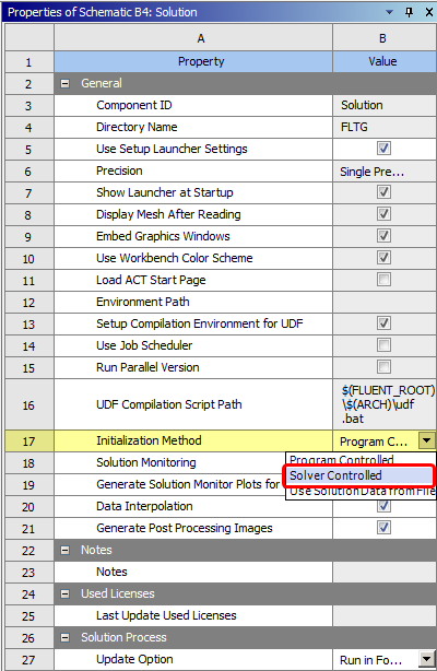
The next time you have modifications to your Fluent project, the 1-Way transient results can be updated from Workbench and the Fluent GUI can be closed.
See Also:
When coupling Rocky with Ansys Fluent or when using Rocky with Ansys Workbench, special components must be installed. Use the sections below to help you determine what components you need for which Ansys product, and how to install them.
Use this procedure if you want to use the 1-Way Fluent (see also About Using the 1-Way Fluent Method), the 2-Way Fluent (see also About Using the 2-Way Fluent Method), or the 2-Way Fluent Semi-Resolved (see also About Using the 2-Way Fluent Semi-Resolved Method) coupling method for your simulations without going through Ansys Workbench, but are not certain whether you have installed the Ansys Fluent Coupling Support component during your initial Rocky installation (Figure 1).

Use this procedure if you want to use the 1-Way Fluent (see also About Using the 1-Way Fluent Method) coupling method through Ansys Workbench (which also requires a geometry from Ansys SpaceClaim) but are not certain whether you have installed both the Ansys Fluent Coupling Support (Figure 1) and Ansys Workbench Addin (Figure 2) components during your initial Rocky installation.
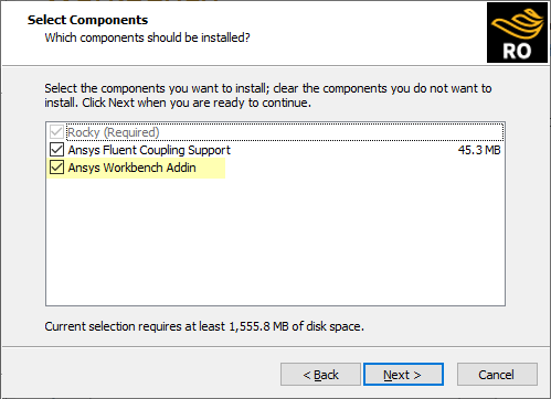
Use this procedure if you want to use Ansys Mechanical through Workbench (which also requires a geometry from Ansys SpaceClaim, see also About Rocky and Ansys Mechanical Integration) with Rocky, and are unsure whether you have installed Ansys Workbench Addin (Figure 2) component during your initial Rocky installation.
For Windows machines, reinstall Rocky and ensure that the Ansys Workbench Addin component remains selected during installation.
See Also:
From the Rocky Options menu, point to Ansys and then click Uninstall Fluent/Rocky export.
See Also:
The 2-Way Fluent method enables you to both send Rocky particle flow data to and accept fluid data from Ansys Fluent. It is considered to be an unresolved method.
Note: There are no special components that must be installed in Rocky for conducting a 2-Way coupled simulation with Fluent.
What would you like to do?
Learn more About Using the 2-Way Fluent Method
Exchange Rocky Particle Data with Fluid Flow Data from Ansys Fluent, which covers only the final coupling portion of the entire 2-Way Fluent Coupling procedure.
Use the 2-Way Fluent Method to Process a Fluent and Rocky Simulation, which covers the full procedure, including the setup steps that are required in Fluent.
See Also:
The 2-Way Fluent Method is an unresolved CFD Coupling option that enables Rocky to receive fluid flow data from Ansys Fluent, calculate how the fluid movement affects the particle flow, and then send the momentum (and other quantities) sources back to Fluent for Fluent to calculate the fluid flow for the next timestep. 2-Way Fluent coupling results in a Rocky simulation that fully depicts how particles and fluids interact with each other in the confines of the equipment.
Tip: If your application requires a very refined Fluent mesh in order to accurately simulate the fluid flow behavior, and the resulting fluid cell sizes are many times smaller than the particle size itself, you might want to instead consider using the 2-Way Fluent Semi-Resolved Method.
To make it possible to share the Fluent fluid flow data with Rocky, Rocky includes a special Ansys Fluent Coupling Support component. This component is included by default during your Rocky installation but if for some reason is not included or is in need of being updated, it can be installed later through the Rocky UI. (See also Install Ansys Coupling Components.)
In addition, 2-Way coupling requires that a Rocky-supported version of Ansys Fluent is installed upon the same machine that contains your Rocky program installation. (See also System Requirements.)
2-Way Fluent coupled simulations require that the initial CFD simulation be set up a certain way in Fluent to ensure that it works correctly when coupled with Rocky. These required settings are outlined in the accompanying procedure Use the 2-Way Fluent Method to Process Fluent and Rocky Simulations, and more detailed information about the Fluent settings can be found in the CFD Coupling Technical Manual manual (from the Rocky Help menu, point to Manuals and then click CFD Coupling Technical Manual.)
There are many ways you can customize your coupled simulations. For example, you can measure heat exchange by using thermal modeling, can choose to begin your simulation empty or with particles and/or fluid velocities already in the system, and can use the same or different geometry files in both programs.
Note: In this version of Rocky, there are no restrictions on the type of Energy Equation you define in Fluent.
Use the sections below to learn more about setting up your case in Fluent for later 2-way coupling with Rocky.
Both single phase and multiphase approaches are supported using the 2-Way Fluent CFD Coupling method. Single phase is defined as one CFD fluid phase plus one DEM particle phase. Multiphase (or multi-phase) is defined as two or more CFD fluid phases plus one DEM particle phase.
Important: Since these phases are defined in Ansys Fluent, and this user manual's purpose is to cover only Rocky product usage, most of the information provided in this document will apply to both approaches. However, differences will be specified when critical to the understanding of Rocky-Fluent product interactions.
About the Single Phase Approach The single phase approach is faster than the equivalent simulation using the multiphase approach. It is also easier to set up and allows for a broader range of models.
About the Multiphase Approach In this version of Rocky, the following three types of Turbulence Multiphase Model you define for your multiphase Fluent case are supported in 2-Way Fluent simulations:
Mixture
Dispersed
Per Phase
These turbulence models are also compatible with sub-stepping. (See Sub-Stepping definition in Table 2 below.)
User Defined Memories (UDMs) are supported, as well as mesh interface zones. If a Fluent case has additional UDFs beyond those used for Rocky, Rocky will copy (and if only the source files are provided, compile) the additional UDFs to the coupled project as long as the below requirements are met. (See also additional information in the Rocky CFD Coupling Technical Manual.)
UDF Usage Requirements: There are several requirements in order to make use of UDFs, as listed below:
You must place all UDF files in the same folder in which your Fluent CAS (CAS.H5 or CAS.GZ) file is located. Rocky will then copy those files to the simulation folder and use them during the 2-Way coupling simulation.
You must provide the UDF files via one of the following two methods:
By providing the source files. (E.g., the .c, .h, and .cpp source and header files.) In this case, you must launch Rocky from an environment that has all the necessary variables for UDF compilation.
Tip: An easy way to accomplish this is to open a command prompt and then call the
udf.batfile, which in Windows, is usually located in the following folderC:Program Files\ANSYS Inc\ {version}\fluent\ntbin\win64Following this step, you can then launch Rocky from the command prompt. (See also Appendix G: Perform Tasks from the Command Line or Journal.)Recommended: By providing the folder containing the UDF binary files, you must have already compiled the UDF and there are no requirements in terms of the environment variables.
Important: Ensure that you do not change nor replace any rocky source functions, as this might affect the coupling behavior.
In this version of Rocky, you may define within your Fluent CAS (CAS.H5 or CAS.GZ) file source terms, such as momentum, via journal. During the coupled simulation, Rocky will keep these source terms and will add its own source terms on top of the ones you defined in Fluent.
Rocky will also support importing multiple Fluent Moving Meshes during the setup of a 2-Way Fluent coupling simulation, which enables you to see simple translation or rotation movements on both the Rocky and Fluent sides. (See also About Creating and Applying Motion Frames.)
Note: In this version of Rocky, moving meshes are now compatible with sub-stepping. (See also Sub-Stepping definition in Table 2 below.)
This version of Rocky supports 2-Way coupling with Fluent cases that are defined with multiple species (multi-species). In these cases, Fluent shares species information with Rocky and Rocky sends the resulting mass source terms back to Fluent. This allows you to simulate particle-fluid interactions on the individual chemical components within a fluid mixture, thereby making it possible for you to study chemical reactions such as combustion, crystallization, and more.
This ability is possible only when used in combination with an external module that supports these computations. This can be a ready-to-use module—such as the CFD-Coupled Particle Crystallization or the CFD-Coupled Particle Combustion module—or a module you create yourself using Rocky's API:Solver functionality. (To learn more, from the Help menu, point to Manuals and then click API:Solver Manual.)
As illustrated in Figure 1, when multiple species are enabled within your Fluent case, the following three variables are sent from Fluent to Rocky per species:
Mole Fraction
Mass Diffusivity
Molecular Weight
During processing, Rocky sends back to Fluent mass source terms for all but the last species that you specified in the Fluent case, and Fluent will use this information to close the mass balance. Thus, what you set for the last species in your Fluent setup is very important as Fluent considers it to be the bulk species. This last species, therefore, will not result in a mass source term from Rocky. If needed, you can infer the mass source for the final species by subtracting the others from the total.
Figure 3.226: Illustration showing Fluent species information (left, red box) being shared with Rocky (right, red box) during 2-Way Fluent setup. Later during processing, Rocky sends mass source terms (right, blue box) back to Fluent for all but the last species in the list.
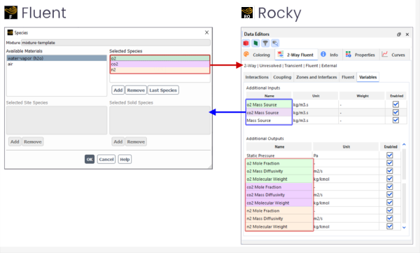
For more information about these variables, see the About Additional Input and Output Variables section below.
Tip: For a brief overview of this functionality, refer to the video Simulate Chemical Reactions in Rocky on the Tips and Tricks page of the Customer Portal.
When setting 2-Way Fluent CFD Coupling, Rocky will ask you for two kinds of files that you create as part of your initial Fluent setup: a CAS (CAS.H5 or CAS.GZ) file, which contains the initial CFD simulation setting you created in Fluent, and an optional DAT (DAT.H5 or DAT.GZ) file, which contains initial flow field data for the fluid.
Since Fluent 2020 R1, the standard format (Common Fluid Format (CFF)) for case files is CAS.H5 and DAT.H5.
However, these files are not as fully compatible with post-processing in Fluent as were the legacy format of CAS.GZ and DAT.GZ.
Therefore, an additional file with the format FLPRJ is required by CFD-Post in order to load the transient results from
the Fluent simulation. This is achieved by using Fluent's auto-save feature, which writes the .cas.h5, .dat.h5, and also the .flprj files, all of which
ensures the files are fully compatible with CFD-Post.
During the coupled simulation, Rocky will write another set of CAS.H5 and DAT.H5 files
that allow you to restart and resume the Rocky simulation. Specifically, when you provide Rocky with the Fluent files, Rocky makes copies of them in an
internal "file" folder within your project folder, and renames them: the CAS (CAS.H5 or CAS.GZ) file becomes "two_way_coupling" and the
DAT (DAT.H5 or DAT.GZ) file becomes "with_particles". Therefore, the filenames two_way_coupling.cas, two_way_coupling.cas.h5, and
two_way_coupling.cas.gz are reserved names by Rocky and they are not allowed in the Fluent auto-save function.
Important: Be aware that Fluent case files with the aforementioned reserved names will be blocked.
Tip:In order to save space in your storage system and not duplicate the CAS.H5 and DAT.H5 files unnecessarily, it is recommended that
you disable the Keep all files option and keep only the last 2 (or more) files. (See also the Fluent Files and Storage section below.)
Later when you run or process the coupled simulation, Rocky adds components to these files and moves them to another "rocky\files" folder within your project folder. These are the files that will be used to generate the coupled simulation.
If at some point you want to modify the CAS (CAS.H5 or CAS.GZ) file, you can do so one of two ways:
From inside Rocky, you can click Open on the 2-Way Fluent | Fluent tab, which opens the Rocky "two_way_coupling" version of the file inside Fluent, which you can then modify. When you are ready to save your changes, you must keep the name and location exactly as it was when you opened it, otherwise Rocky will not be able to recognize the changes. When the changes are saved, you can click Refresh in Rocky to include them.
From inside Fluent, you can modify and save your original CAS (CAS.H5 or CAS.GZ) file. If you do this, you will have to restart the coupling process in Rocky by first selecting No Coupling from the CFD Coupling Mode list, and then following the steps to re-couple your Rocky simulation to the updated CAS (CAS.H5 or CAS.GZ) file.
Once your Fluent case is defined and you are ready to set up your 2-way coupled simulation in Rocky, there are several different options that can help you achieve your goals. Use the sections below to learn more.
Some external modules might require certain variables or data to be exchanged with Fluent during the coupled simulation. In this version of Rocky, these additional input and output variables are applicable only with Fluent cases with species transfer enabled and which contains a mixture of various fluids.
For these special types of Fluent cases only, Rocky will display after Fluent case validation some additional variables on its Variables tab (Figures 1 and 12). On the Variables tab, Additional Inputs lists items that Fluent will receive from Rocky during the simulation, which Rocky instructs Fluent to create as User Defined Memories (UDMs). And Additional Outputs lists the items that Fluent will share during the simulation with Rocky.
Both types of additional variables can be viewed as Fluid properties in Rocky after processing, but note that they will not be calculated unless an external module is enabled that makes use of those variables. (Refer to your module's documentation for additional information.)
In order for 2-Way Fluent simulations to be compatible with saving the project for tasks such as the three listed below, the Simulation Output Frequency setting on the Solver | Time tab is disabled and a new Fluent Outputs Multiplier parameter is provided. (See also About Solver Parameters.)
Saving a simulation for restart purposes (see also Save a Copy of a Partially Processed Simulation for Restart Purposes)
Resuming a simulation (Resume Processing a Stopped Simulation)
Extending the duration of a simulation (see also About Extending the Duration of an In-Process or Completed Simulation)
Rocky uses the Time Step Size value that you set in Fluent to determine the initial Output Frequency of the Rocky and Fluent files. Rocky automatically adjusts its output frequency to match the time step set in the Fluent case. This means that by default, for every Fluent time step, one Rocky file and one Fluent file will be outputted.
You can change the frequency of outputs by using the Fluent Outputs Multiplier. A higher multiplier will result in fewer Rocky and Fluent files.
In addition to the Fluent Outputs Multiplier, you are also given the option to Keep all files or determine how many of the last-saved DAT (and in some cases, as with moving meshes, CAS) Files to keep, which can help you manage your Fluent file storage.
Even if you increase your Fluent Output Multiplier, keeping all files is not always recommended for the 2-Way Fluent method due to the often large size of the Fluent mesh files. Unless you require the full set of files for post-processing in Fluent, it is recommended that you save only the last two (or more) Fluent files.
Important: If you decide to save fewer than all of the files, be aware that you will not be able to post-process the unsaved files in Fluent. Also, be aware that the number of DAT (and sometimes CAS) files you save will be as far back in time as you can restart your simulation since fluid data will not be available for prior times.
Tip: You can also choose which quantities and frequency you want to write to disk using Fluent's Autosave functionality.
If Volumetric Diffusion is selected for Mapping Method, then every iteration the volumetric diffusion equation is applied to the mesh. Rocky then decides if more iterations are required based upon the following criteria:
Target Maximum Volume Fraction

Maximum Iterations

See Figure 2 below for an illustration.
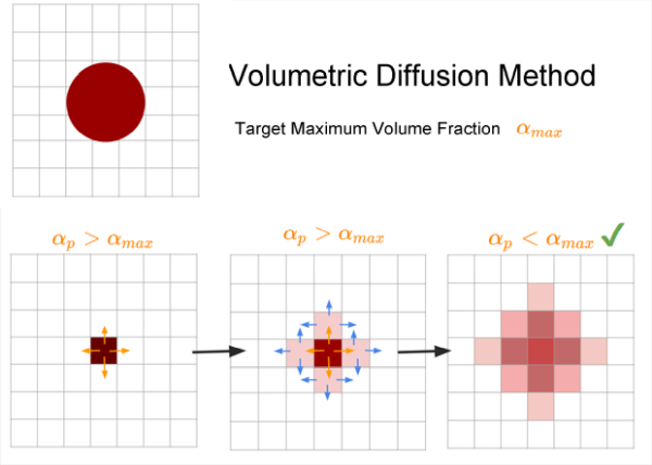
Tip: When Rocky's Advanced Features are enabled (see About Setting Global Preferences), these paraeters are available for tuning.
In this version of Rocky, you are able to select which interfaces you want to perform mapping across. This enables you to choose whether the averaging procedure will take into account CFD cells that are located on the opposite side of the interface or only on the same side of the interface as the cells (Figure 3).
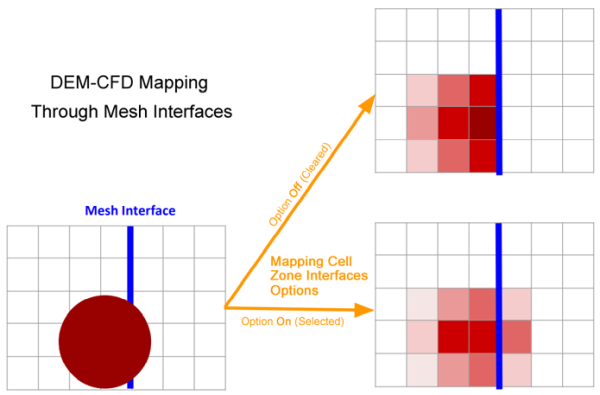
For example, if the interface in question is not a physical boundary, and you created it because the case had sliding meshes or you simply decomposed the mesh in order to get a better quality, you may not want to block the transferring of the volume to the other side and in this case, would want to select the Mapping Cell Zone Interfaces option for that interface.
However, there may also be cases where you do not want to transfer the forces and volume fraction to the other side. For example, if in the CFD solver the interface is modeling a perforated plate or a grate, this should block particles from crossing the interface and therefore you can avoid the transferring of that volume by ensuring the Mapping Cell Zone Interfaces option is cleared for that interface.
Some best practices for using this method include:
Avoid discontinuous volume fraction field and momentum and energy source terms near interfaces
Avoid high volume fraction values
A shadow boundary is an internal boundary without thickness. Due to the way Rocky optimizes the representation of the CFD domain in order to increase the simulation speed, in rare situations particles may be placed in a neighboring cell when the L-E mapping is performed. This is not a problem in the great majority of cases; however, when such a thing happens near a shadow boundary, there is a small chance that the particle is misplaced on the wrong side of the boundary. In order to avoid this chance occurrence, Rocky will prevent coupled simulations from processing if they have polygonal cells at shadow boundaries.
To get around this limitation, add a thickness to your shadow boundaries, or avoid using polyhedron meshes around them.
In this version of Rocky, you are able to visualize in a 3D View window the transient fluid flow data represented by Nodes and/or Vectors. This display, when combined with Particle visualization, can provide you a fuller visual confirmation of your dynamic 2-Way coupled simulation (Figure 4).
Figure 3.229: Example of a 2-Way Fluent simulation showing transient fluid flow vectors (in purple), and transient particle nodes (all colors)
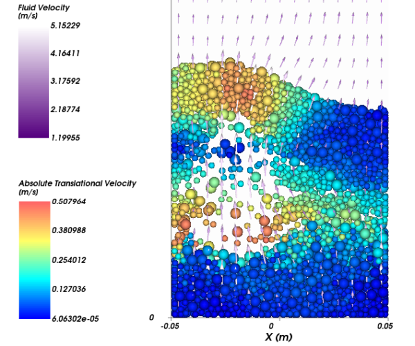
(See also About Using the Coloring Tab to Change a 3D View and About Properties.)
In this version of Rocky, you are able to set torque and lift laws for Unresolved 2-way coupling with Fluent Figure 3.230: Lift and Torque Laws in the Data Editors panel. All the current lift and torque laws are available, however they are suitable only for spherical particles and very dilute flows.
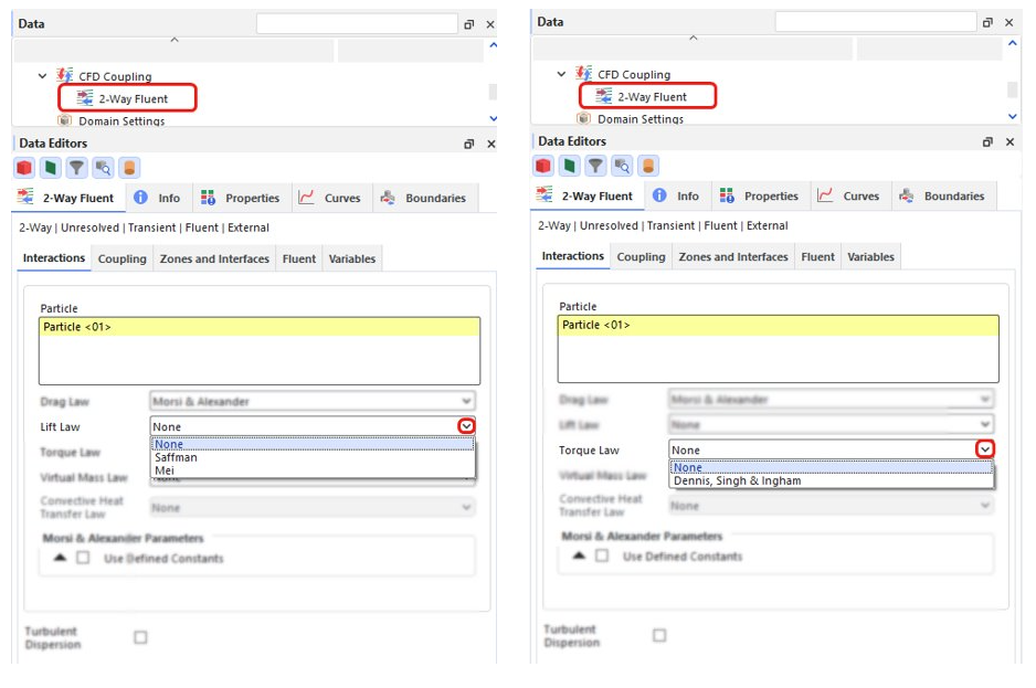
After processing your simulation, the referred properties will show up inside Particles in the Properties tab Figure 3.231: Lift and Torque Laws in the Data Editors panel after processing your simulation.
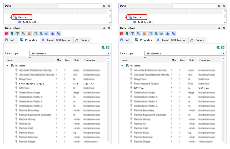
Shell and Solid particles composed of Multiple Elements (also known as meshed or flexible particles) are incompatible with 2-Way Fluent CFD Coupling. The only flexible particle shapes compatible with this feature are Fibers. (See also About Adding and Editing Particle Sets.)
In addition, Shell particles composed of Single Elements (also known as "rigid" particles) are also incompatible with 2-Way Fluent CFD Coupling.
Also, note that when combined with Coarse Grain models, only drag forces are considered. This means that other non-drag fluid force models, such as virtual mass and lift, are incompatible with Coarse Grain modeling.
For a full list of limitations, refer to the Ansys and CFD Coupling Limitations topic.
Use the images and tables below to help you understand how to set up the Rocky portion of the 2-Way Fluent method. Further details can be found in the following resources:
CFD Coupling Technical Manual document (from the Help menu, point to Manuals, and then click CFD Coupling Technical Manual).
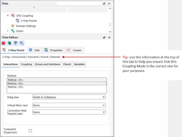
Table 1: 2-Way Fluent, Interactions Tab Settings
Setting | Description | Range |
|---|---|---|
Particle | Permits correlations- such as drag, virtual mass, and convective heat transfer laws (if applicable)- to be defined per Particle set. You accomplish this by selecting (or multi-selecting) from a list of previously defined Particle sets, and then defining the applicable CFD Laws for only the selected set (or sets). Important: Even though they will still be listed here, neither flexible Shell nor flexible Solid particle shapes are supported in CFD Coupling approaches, including this one. (See also Ansys and CFD Coupling Limitations). | Automatically provided |
Drag Law | Correlation used by Rocky to calculate drag forces on particles. Note: With the exception of Ganser, which is incompatible with Assembly, concave and Shell particle shapes (see also About Adding and Editing Particle Sets), these drag laws apply to any supported particle shapes (see also Ansys and CFD Coupling Limitations) except Fiber and also Solid Sphero-Cylinder shapes, which have their own modified drag law based on the work by Marheineke and Wegener that should always be used for those shapes. Tip: For more information about these laws, refer to the CFD Coupling Technical Manual. (From the Rocky Help menu, point to Manuals, and then click CFD Coupling Technical Manual.) | Wen & Yu; Schiller & Naumann; Haider & Levenspiel; Ganser; Ergun; Gidaspow, Bezburuah & Ding; Huilin & Gidaspow; Di Felice; Dallavalle: Marheineke & Wegener; Syamlal & O'Brien; Morsi & Alexander; Hill, Koch & Ladd; Hill & Koch Note: If you have an external Module that adds in an additional CFD law, you must use that law at least once in your simulation project if the Module is enabled. Refer to the Module's documentation (if provided) for more information. (See also Rocky Simulation Entities that can be Affected by Modules). |
Lift Law | Correlation used by Rocky to calculate the fluid-particle force transversal to the direction of the relative velocity. | None; Saffman; Mei. |
Torque Law | Correlation used by Rocky to calculate the torque exerted by the fluid over the particle. | None; Dennis, Singh and Ingham. |
Virtual Mass Law | Correlation used by Rocky to calculate the virtual mass coefficient. Tip: For more information about these laws, refer to the CFD Coupling Technical Manual. (From the Rocky Help menu, point to Manuals, and then click CFD Coupling Technical Manual.) | None; Constant; Paladino; Ishii & Mishima Note: If you have an external Module that adds in an additional CFD law, you must use that law at least once in your simulation project if the Module is enabled. Refer to the Module's documentation (if provided) for more information. (See also Rocky Simulation Entities that can be Affected by Modules). |
Convective Heat Transfer Law | When both Thermal Model is enabled (see also About Physics Parameters) and the selected Fluent CAS (CAS.H5 or CAS.GZ) file is set to solve energy equations, this correlation is used by Rocky to calculate the fluid-particle convective heat transfer coefficient. Note: Note: The thermal (energy) solution option must be the same in both Fluent and Rocky setups. | None; Ranz & Marshall; Whitaker; Gunn Note: If you have an external Module that adds in an additional CFD law, you must use that law at least once in your simulation project if the Module is enabled. Refer to the Module's documentation (if provided) for more information. (See also Rocky Simulation Entities that can be Affected by Modules). |
Use Defined Constants | When Morsi & Alexander is selected for Drag Law, this enables you to determine how the model's three coefficients will be determined. Specifically:
| Turns on or off |
| When Use Defined Constants is enabled, this is the value you
want assigned to the | Any value |
| When Use Defined Constants is enabled, this is the value you
want assigned to the | Any value |
| When Use Defined Constants is enabled, this is the value you
want assigned to the | Any value |
Syamlal & O'Brien Parameters c1 | When Syamlal & O'Brien is selected for Drag Law, this defines the c1 coefficient required by the drag law. Tip:For more information about this parameter, refer to the CFD Coupling Technical Manual. (From the Rocky Help menu, point to Manuals, and then click CFD Coupling Technical Manual.) | Any value |
Syamlal & O'Brien Parameters d1 | When Syamlal & O'Brien is selected for Drag Law, this defines the d1 coefficient required by the drag law. Tip:For more information about this parameter, refer to the CFD Coupling Technical Manual. (From the Rocky Help menu, point to Manuals, and then click CFD Coupling Technical Manual.) | Any value |
Turbulent Dispersion | When the imported CAS (CAS.H5 or CAS.GZ) file has a turbulent model that uses turbulence kinetic energy as one of its quantities, this allows those turbulent parameters to be used and modified in Rocky. Clearing this checkbox prevents the turbulent parameters from being used during the Rocky simulation. Tip: For more information about this parameter, refer to the CFD Coupling Technical Manual. (From the Rocky Help menu, point to Manuals, and then click CFD Coupling Technical Manual.) | Turns on or off |


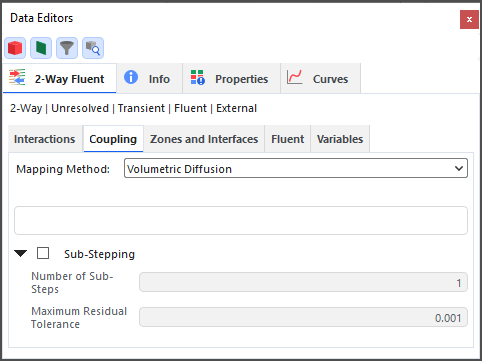
Figure 3.234: CFD Coupling, 2-Way Fluent, Coupling tab when Uniform Distribution is selected for Mapping Method
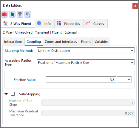
Table 2: 2-Way Fluent, Coupling Tab Settings
Setting | Description | Range |
|---|---|---|
Mapping Method | Helps facilitate smoother Fluent calculations by distributing each particle's information across a specific mesh region. These regions are composed of the Fluent mesh cell where the particle is located and its neighboring cells. The two options for employing this mapping method are as follows:
(See also Figure 1 above.) | Uniform Distribution; Volumetric Diffusion |
Averaging Radius Type | When Uniform Distribution is selected for Mapping Method, this determines what radius around a Fluent mesh cell Rocky will average the neighboring cells' particle information. This step is necessary to ensure smooth calculations for Fluent. The higher the values chosen, the more effective the smoothing but the more time to process. Specifically, choose:
It is recommended that whatever value you choose includes 1-2 additional Fluent mesh cells only. | Fraction of Maximum Particle Size; Absolute Value |
Fraction Value | When Averaging Radius Type is set to Fraction of Maximum Particle Size, this value will be multiplied by the maximum particle size to achieve the averaging radius. | Any value |
Absolute Value | When Averaging Radius Type is set to Absolute Value, this is value will be used as the averaging radius. | Any value |
Maximum Iterations | When the Advanced Features checkbox is enabled on the Options | Preferences dialog (see also About Setting Global Preferences), and Volumetric Diffusion is selected for Mapping Method, the mapping process is interrupted if the Maximum Volume Fraction Target is not achieved during this number of iterations. This parameter has lower precedence than Minimum Iterations above. Note: This text field does not support parametric variables. (See also I cannot enter an input variable or mathematical function into a text field). | Values 10-1000 Tip: The recommended value is 500 Note: Small values of this parameter may result in Rocky not achieving the Maximum Volume Target Fraction you have specified. |
Solids Maximum Volume Fraction Target | When the Advanced Features checkbox is enabled on the Options | Preferences dialog (see also About Setting Global Preferences), and Volumetric Diffusion is selected for Mapping Method, this defines the maximum volume fraction—of only the solids (particles); the fluid is not considered—to be honored during the simulation. | Values greater than 0 (zero) but less than 1 Tip: The recommended values are between 0.6 and 0.85 |
Sub-Stepping | Allows you to choose how often during processing Rocky will interact with Fluent inside a single Fluent time step. Enabling Rocky to interact more frequently with Fluent increases stability and accuracy of the coupled calculations, but can increase the processing time. To counteract these effects, you can combine sub-stepping with a higher Fluent time step to achieve a better balance between processing speed and stability/accuracy. When cleared, Rocky will interact only once with Fluent during each Fluent time step. If enabled, Rocky will interact more than once with Fluent during each Fluent time step. | Turns on or off |
Number of Sub-Steps | When Sub-Stepping is enabled, this defines the number of times Rocky will interact with Fluent during each Fluent time step. | 2 - 50 |
Maximum Residual Tolerance | When Sub-stepping is enabled, Rocky overwrites the residual tolerances defined in the Fluent CAS (CAS.H5 or CAS.GZ) file with this value, which defines the largest allowable value of residual error during each interaction Rocky has with Fluent. The solution is obtained when the residual error during an iteration in any computational node is less than the specified tolerance. | 1e-16 - 1.0 Important: Setting this value enables Rocky to overwrite the residual tolerances defined in the Fluent CAS (CAS.H5 or CAS.GZ) file. |
Overwrite CFD Update Distance | When the Advanced Features checkbox is enabled on the Options | Preferences dialog (see also About Setting Global Preferences), this allows you to overwrite the default distance used as a criteria for updating the volume fraction field. As this step may take a considerable amount of time, increasing the associated CFD Update Distance value (and therefore reducing the frequency at which the volume fraction is updated) might help reduce processing time. | Turns on or off |
CFD Update Distance | When the Advanced Features checkbox is enabled on the Options | Preferences dialog (see also About Setting Global Preferences), and the Overwrite CFD Update Distance checkbox is enabled, this defines the maximum distance the particles are allowed to travel before a volume fraction field update. The smaller the value, the more frequent the update. As this step may take a considerable amount of time, increasing the update distance (and therefore reducing the frequency at which the volume fraction is updated) might help reduce processing time. | Positive values |
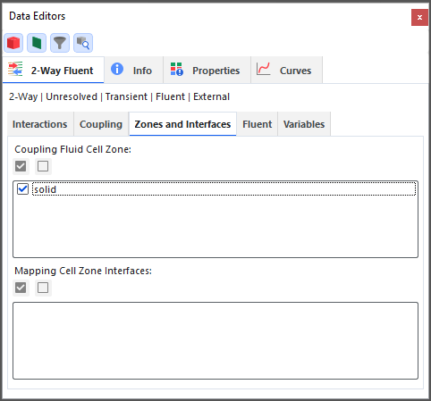
Table 3: 2-Way Fluent, Zones and Interfaces Tab Settings
Setting | Description | Range |
|---|---|---|
Coupling Fluid Cell Zone | Enables you to choose which fluid cell zones you want included in the coupled calculations. Note: At least one fluid zone must be selected in order to process the coupled simulation. | Turns on or off |
Mapping Cell Zone Interfaces | Enables you to select which interfaces you want to perform the mapping across. If selected, the averaging procedure will take into account CFD cells that are located on the other side of the interface, whereas if not selected, the mapping will take into account only cells that are on the same side of the interface as the cell. (See also Figure 2 above.) | Turns on or off |

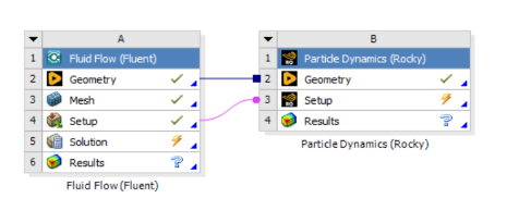
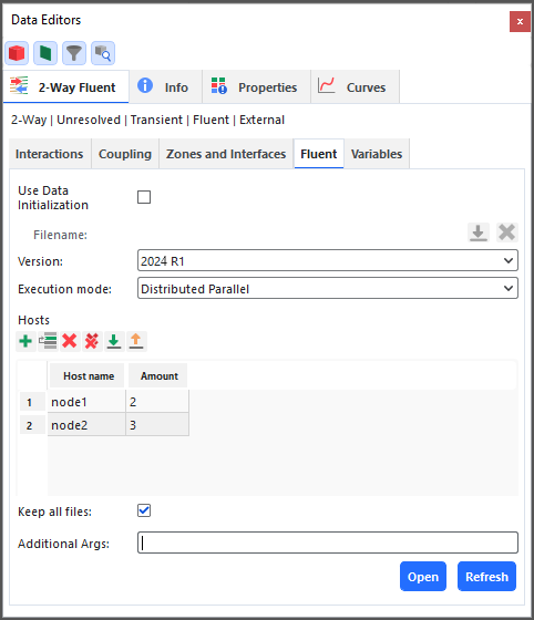
Table 4: 2-Way Fluent, Fluent Tab Settings
Setting | Description | Range |
|---|---|---|
Rocky Phase | For multiphase CAS (CAS.H5 orCAS.GZ) files only, this enables you to choose which secondary phase of the Fluent file represents particle flow information. Note: single phase CFD files will not list this option as the Rocky Phase can be automatically determined. | List automatically generated based upon what secondary phases were entered in the Fluent CAS (CAS.H5 or CAS.GZ) file. |
Use Data Initialization | When selected, enables you to begin your simulation with an initial flow field based upon the Fluent fluid phases. This initial solution is saved from Fluent into a DAT (DAT.H5 or DAT.GZ) file that is then used by Rocky during processing. Important: If you choose to use initial fluid flow data in your simulation, it is important that the secondary phase (particulate phase) has a zero volume fraction. This is calculated in Rocky and sent to Fluent. | Turns on or off |
Version | Enables you to select the Ansys Fluent software version you want to use for processing. Tip: If you do not see the Ansys version you expected, see also Rocky does not list my Ansys version when I try to set up 2-Way Fluent Coupling. | List automatically generated based upon the software versions detected. |
Execution mode | Enables you to select how your computer and/or network will process the fluid portion of the coupled simulation. Note: Regardless of what is selected here, the Rocky portion of the coupled simulation will still be processed according to the Simulation Target and related information that you specified on Solver | General Settings tab (see also About Starting a Simulation. Specifically:
| Serial; Local Parallel; Distributed Parallel |
Solver Processes | When Local Parallel is selected for Execution mode, this enables you to determine the number of computer processors (threads) you want dedicated to the CFD solver. Note: You select the number of processors used by Rocky when you start processing the simulation. (See also About Starting a Simulation.) Note: This text field does not support parametric variables. (See also I cannot enter an input variable or mathematical function into a text field.) | Positive values |
Host Name | When Distributed Parallel is selected for Execution mode, this is the name of the remote machine on your network. Tip:Contact your IT administrator to find out the host names of the fluid nodes on your network. | 99 character limit |
Amount | When Distributed Parallel is selected for Execution mode, for each separate Host Name listed, this is the number of computer processors you want dedicated to the CFD solver. | Positive values |
Keep all files | When selected, all Fluent DAT (DAT.H5 or DAT.GZ) files (and in some cases, as with moving meshes, CAS files as well) will be saved every time a Rocky output file is saved. When cleared, this enables you to select how many DAT (and sometimes CAS) Files to keep. Keeping fewer than all the DAT (and sometimes CAS) files can help you save storage space when processing your simulation. However, doing so can also limit your fluid post-processing abilities, as well as your ability to restart the simulation from an earlier time due to the reduced amount of past fluid data that is available when you save fewer DAT (and sometimes CAS) files. | Turns on or off |
Files to keep | When Keep all files is cleared, this determines how many Fluent DAT (DAT.H5 or DAT.GZ) files (and in some cases, as with moving meshes, CAS files as well) are saved with each Rocky output file saved. For example, if set to 1, only the last DAT (and sometimes CAS) file will be kept. If set to 2, only the last 2 DAT (and sometimes CAS) files will be kept, and so on. This setting can be useful in cases where you need only to keep files past steady state, for example, or when you do not require the Fluent files for post-processing. Important: If you decide to save fewer than all of the files, the number of DAT (and sometimes CAS) files you save will be as far back in time as you can restart your simulation since fluid data will not be available for prior times. Note: This text field does not support parametric variables. (See also I cannot enter an input variable or mathematical function into a text field.) | Whole values greater than or equal to 1 |
Additional Args | This displays the set of arguments that Rocky passed "as-is" from the Fluent command line when the coupled simulation began. For advanced users, this enables more control of the Fluent portion of the processing. For more information about these arguments, see your Ansys Fluent documentation. | Positive values |
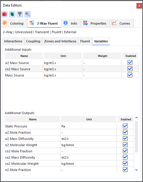
Table 5: 2-Way Fluent, Variables Tab Display
Property | Display Description |
|---|---|
Additional Inputs | |
Name | The name of the additional variable or data that Fluent will receive from Rocky during the simulation. Each Additional Input has a corresponding UDM in Fluent. |
Unit | The SI unit of the variable. |
Weight | The name of the variable that will be used as a weight for the selected averaging method. This variable can be another Additional Input or Additional Output variable, or can be a standard variable in Rocky, such as Fluid Velocity. |
Additional Outputs | |
Name | The name of the additional variable or data that Fluent will share with Rocky during the simulation. |
Unit | The SI unit of the variable. |
What would you like to do?
Exchange Rocky Particle Data with Fluid Flow Data from Ansys Fluent, which covers only the final coupling portion of the entire 2-Way Fluent Coupling procedure.
Use the 2-Way Fluent Method to Process a Fluent and Rocky Simulation, which covers the full procedure, including the setup steps that are required in Fluent.
See Also
Before starting the 2-way coupled run, you must initialize the CFD flow field in the entire CFD domain. When setting up a 2-way coupling simulation between Rocky and Fluent in Workbench, there are two options to set initial values for the flow variables, and initialize the solution using these values:
1.Initialize with values from the case.
The values set in the Solution Initialization task page from Fluent will be used to generate the initial fluid flow field. These fluid values can be computed from information in a specified zone, entered manually, or computed based on all zones by the solver.
2.Use existing solution data.
The desired information is automatically imported from the Fluent case that already run and used as the initial flow field for the coupled run.
You can use this option to facilitate convergence of the coupled simulation by providing a converged flow field without particles, or provide different values for particular variables, such as temperature or phase volume fraction, into different cells using the Patch option in Fluent.
The coupled simulation will initialize the fluid field using the values set in the Solution Initialization task page from Fluent if only the Setup entry from the Fluid Flow Field is linked to the Particle Dynamics Setup.
Figure 3.240: 2-way Coupled Rocky-Fluent simulation in Workbench initializing the fluid field using the values set in the Fluent setup
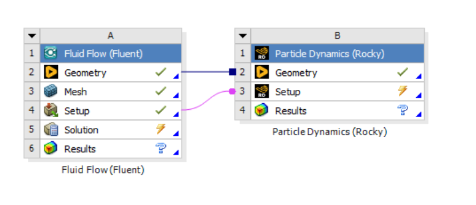
The Fluent tab of the 2-Way Fluent editor will have the option Use Data Initialization unchecked and blocked.
Figure 3.241: Fluent tab in Rocky Data Editors when coupling within workbench without initial fluid data file
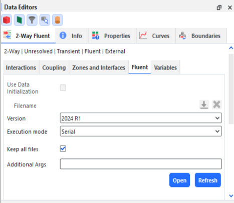
The coupled simulation will use the existing fluid data if the Setup and Solution entries from the Fluid Flow Field are linked to the Particle Dynamics Setup.
Figure 3.242: 2-way Coupled Rocky-Fluent simulation in Workbench initializing the fluid field using an initial fluid field data
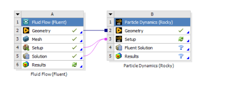
The Fluent tab of the 2-Way Fluent editor will contain the Use Data Initialization checked and the Filename of the initial data that was imported into the coupled simulation.
Figure 3.243: Fluent tab in Rocky Data Editors with existing fluid data is used in a 2-way coupled simulation
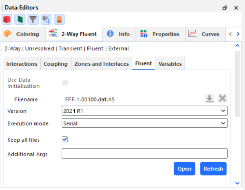
Tip: This procedure covers only the final coupling portion of the entire 2-Way Fluent Coupling procedure, which applies to both multiphase and single phase coupling methods. To see the full procedure, including the setup steps that are required in Fluent, refer instead to Use the 2-Way Fluent Method to Process Fluent and Rocky Simulations.
Important: Ensure that you have a Rocky-supported version of Ansys Fluent installed upon the same machine that contains your Rocky program installation. (See also System Requirements.) Note: If you are not certain whether you have installed the Ansys Fluent Coupling Support component during your Rocky installation, first follow the Install Ansys Coupling Components procedure before beginning these steps.
From the Data panel, click CFD Coupling and then from the Data Editors panel, choose Fluent from the Coupling Mode list.
From the Select Fluent CAS file dialog, locate and select the CAS (CAS.H5 or CAS.GZ) file you previously generated in Fluent, and then click Open. Important: A mesh validation step will occur immediately after the CAS file import. This requires a valid Fluent license on the same machine upon which you are running the Rocky simulation. After successful import, a new 2-Way Fluent item appears beneath CFD Coupling in the Data panel. In addition, if you chose to set up Moving Meshes in Fluent, one new Frame will appear under Motion Frames in the Data panel for each Cell Zone with motions you have defined. Important: If you have defined your Moving Meshes in Fluent using expressions, Rocky will not be able to create the associated Motion Frames for you automatically. Rather, you must manually create your own Motion Frames in Rocky to match the Fluent motions as closely as possible.
If the CAS (CAS.H5 or CAS.GZ) imported new Motion Frames (or you have created them yourself manually), assign each new Frame to the geometry component you want to share corresponding movements with Fluent. (See also Apply a Motion Frame to an Imported Geometry.)
From the Data panel under CFD Coupling, select the new 2-Way Fluent item and then from the Data Editors panel, do the following:
From the Interactions tab, define the CFD laws you want per Particle set by selecting (or multi-selecting) the set name(s) from the Particle list, and then defining the laws you want for the selected set(s). From this tab, you can also set the Turbulent Dispersion options for the entire coupled simulation. (See also About Using the 2-Way Fluent Method.)
From the Coupling tab, define the Mapping Method and Sub-Stepping options you want.
From the Zones and Interfaces tab, do the following:
Select one or more options from the Coupling Fluid Cell Zone list.
(Optional) If provided, select the options you want from the Mapping Cell Zone Interfaces list.
From the Fluent tab, do all of the following:
Important: If your Fluent case is multiphase, from the Rocky Phase list, ensure that the phase representing particle flow is chosen.
Choose what fluid flow data Rocky starts with by doing one of the following:
To start your Rocky simulation without providing initial flow field data for the fluid, ensure the Use Data Initialization checkbox remains cleared. Doing so ensures that the initialization settings prescribed in Fluent will be used to generate the initial fluid flow.
To start your Rocky simulation with initial fluid flow data, select Use Data Initialization, click the Import File button, and then select and open the DAT (DAT.H5 or DAT.GZ) file you saved in Step II. Important: If you chose to use initial fluid flow data in your simulation and your simulation is multiphase, you must have ensured that the secondary phase (particulate phase) had a volume fraction of zero set before you saved your DAT (DAT.H5 or DAT.GZ) file. This is important because later, after the simulation is initialized, the initial particulate volume fraction will be calculated in Rocky according to the particles enabled at the beginning of the simulation.
From the Version list, select what Ansys version you want to use for fluid coupling. Tip:If you do not see the Ansys version you expected, see also Rocky does not list my Ansys version when I try to set up 2-Way Fluent Coupling.
Choose how the fluid portion of the simulation is processed by doing one of the following:
To have it processed on only one processor on your local machine, from the Execution mode list, select Serial.
To have it processed on multiple processors on your local machine, from the Execution mode list, select Local Parallel and then from the Solver Processes field, enter the number of processors you want to dedicate to the CFD solver.
To have it processed across several machines on your network, from the Execution mode list, select Distributed Parallel and then do one of the following:
Under Hosts, click the Add button for each server you want to add and then for each row, define the Host name and Amount information.
To import an external list of hosts and amounts that you created outside of Rocky, click the Import File button, and then from the Import dialog, locate and select the TXT file containing the information, and then click Open. The Host section is populated with the information from the TXT file. Tip:The format for the TXT file needs to include the Host name repeated on separate lines for each Amount you want devoted. To see an example, create a few sample rows as specified directly above, click Export File and then save and view the results as a TXT file.
Choose how many Fluent files to keep by doing one of the following:
To keep each Fluent DAT (DAT.H5 or DAT.GZ) file (and in some cases, as with moving meshes, CAS files as well) for every Rocky output file that is saved, enable the Keep all files checkbox. Important: Unless you require all files for post-processing in Fluent, keeping all files is not recommended for the 2-Way Fluent method. (See also About Using the 2-Way Fluent Method.)
To keep only the last (or last several) Fluent DAT (DAT.H5 or DAT.GZ) (and sometimes CAS) files saved, ensure the Keep all files checkbox is cleared, and then enter the number of last-saved files you want to keep in the Files to keep box. Tip:Keeping the last 2 (or more) files is recommended. Important: If you decide to save fewer than all of the files, be aware that you will not be able to post-process the unsaved files in Fluent. Also, be aware that the number of DAT (and sometimes CAS) files you save will be as far back in time as you can restart your simulation since fluid data will not be available for prior times. Tip:You can also choose which quantities and frequency you want to write to disk using Fluent's Autosave functionality.
From the Variables tab, review the Additional Inputs and Additional Outputs (if applicable) that Rocky and Fluent will exchange during the coupled simulation.
Tips:
To verify or change the CAS (CAS.H5 or CAS.GZ) file selected, click Open (at the bottom of the 2-Way Fluent | Fluent tab) and Rocky will open its own copy of the CAS (CAS.H5 or CAS.GZ) file in Fluent. From here, you can view or make changes to the Rocky copy of the file. Important: Because Rocky uses only its own copy of the imported CAS (CAS.H5 or CAS.GZ) file, it is critical that you only open the imported CAS (CAS.H5 or CAS.GZ) from Rocky's Open button, and that you save any changes to the default location Rocky indicates.
If you make changes to the Rocky copy of the CAS (CAS.H5 or CAS.GZ) file in Fluent, click Refresh to have Rocky include the updates. Important: The Refresh button works only if you first opened the CAS (CAS.H5 or CAS.GZ) file from the Rocky Open button located at the bottom of the 2-Way Fluent | Fluent tab.
If you made changes to your original Fluent version of the CAS (CAS.H5 or CAS.GZ) file and did not use the Rocky Open button as specified above, you must set the CFD Coupling option to No Coupling to clear the values, and then restart this procedure again from the beginning, selecting the updated CAS (CAS.H5 or CAS.GZ) file in step 3.
Keeping in mind the Time Step Size value you set in Fluent, from the Data panel, click Solver and then from the Data Editors panel, select the Time tab and ensure that what you want is set for Fluent Outputs Multiplier. (See also About Solver Parameters.) Tip:You can see how what you entered affects Rocky's Output Frequency in the disabled Simulation field.
See Also:
The 2-Way Fluent Semi-Resolved Method is a CFD Coupling option that is especially designed to be used with very large (when compared to the cell size of the Fluent mesh) particles that are interacting with a dynamic fluid whose cell mesh is many times smaller than the particle size. It is most useful in cases where the resolution of the fluid flow around the particles is critical to capturing the behavior of your particles.
Note: There are no special components that must be installed in Rocky for conducting a 2-Way coupled simulation with Fluent.
What would you like to do?
Learn more About Using the 2-Way Fluent Semi-Resolved Method
Exchange (2-Way) Rocky Particle Data with Semi-Resolved Fluid Flow Data from Ansys Fluent, which covers only the final coupling portion of the entire 2-Way Fluent Coupling procedure.
Use the 2-Way Fluent Semi-Resolved Method to Process a Fluent and Rocky Simulation, which covers the full procedure, including the setup steps that are required in Fluent.
See Also:
The 2-Way Fluent Semi-Resolved Method is a CFD Coupling option that is similar to the standard, 2-Way Fluent Method but rather than relying on standard correlations for fluid forces based on the centroid fluid velocity and velocity gradients, fluid forces are integrated at the particle's surface. This requires a very fine mesh around the particle in order to work properly.
This method is therefore designed to be used with very large (when compared to the cell size of the Fluent mesh) particles, that are interacting with a dynamic fluid whose cell mesh is many times smaller than the particle size. It is most useful in cases where the resolution of the fluid flow around the particles is critical to capturing the particle behavior.
When determining which 2-Way Fluent method to use, consider the following questions:
Does your application require a very refined Fluent mesh in order to accurately simulate the fluid flow behavior?
Are you able to define your Fluent mesh without the use of polyhedral (including CutCell type) cells? (Can you use either tetrahedrons, prisms, pyramids, or hexahedrons?)
Does your coupled simulation require particles that are at least 10 times larger than the size of the fluid mesh cell?
Do you plan to have fewer than 1000 total particles in your coupled simulation?
Do you plan to use only Spheres, Shells (either rigid or flexible), or Custom Imported Polyhedrons (rigid only) for your particle shapes?
Are you able to get the results you need without the use of the CFD Coupling Particle Statistics module?
If the answers to all of the statements above are "yes", then the semi-resolved method might be the best method for your coupled simulation.
If you answered "no" to any of the questions above, the standard 2-Way Fluent Method might work better for your needs.
Use the information in the sections below to learn more about using the 2-Way Fluent Semi-Resolved Method.
Similar to the standard 2-Way Fluent Method, the 2-Way Semi-Resolved method supports both single and multiphase approaches. It is also similar in regards to the files and formats used.
Refer to the related sections in the About Using the 2-Way Fluent Method topic for details.
Unlike the standard 2-Way Fluent Method, the 2-Way Fluent Semi-Resolved method does not currently support the following abilities:
Post-processing (within Rocky) of fluid-related Properties (Fluid Density, Fluid Velocity, Fluid Viscosity, etc.). (See also About Properties.)
Thermal Coupling: heat exchange using thermal modeling.(See also Enable Thermal Modeling Calculations.)
Assembly particle shapes, Fibers (both rigid and flexible), default Solid particle shapes, and flexible custom imported Polyhedron particle shapes. (See also Rocky Particle Shapes and Capabilities.)
The CFD Coupling Particle Statistics Module. (See also About the CFD Coupling Particle Statistics Module.) Because the 2-Way Fluent Semi-Resolved method does not compute the forces individually, this module when enabled will not return the fluid forces.
Turbulent fluid flows.
Periodic Domain.
Unlike the standard 2-Way Fluent method, the 2-Way Fluent Semi-Resolved method does not use the Time Step Size value that you set in Fluent to determine the initial Output Frequency of the Rocky files. This means that it is possible to have your Fluent outputs and your Rocky outputs happen at different times and frequencies, which might affect your ability to post-process the resulting data in both programs.
If you wish for your Rocky data and your Fluent data to better match in both programs, it is best to ensure that the Time Step Size in Fluent and the Output Settings | Time Interval value in Rocky are multiples.
When Shell particles (either rigid or flexible) are used in 2-Way Fluent Semi-Resolved cases, Rocky calculates buoyancy forces using the gravity direction and the pressure gradient on both sides of the particle.
Note: For the other particle types, the buoyancy is calculated together with the integration of pressure forces.
Similar to the standard 2-Way Fluent Method, you are given the option to Keep all files or determine how many of the last-saved DAT (and in some cases, as with moving meshes, CAS) Files to keep, which can help you manage your Fluent file storage.
Keeping all files is not recommended for the 2-Way Fluent Semi-Resolved method because the Fluent mesh files used in this coupling method are typically much larger than with other methods, which takes up more storage space per file.
Unless you require the full set of files for post-processing in Fluent, it is recommended that you save only the last two (or more) Fluent files.
Important: If you decide to save fewer than all of the files, be aware that you will not be able to post-process the unsaved files in Fluent. Also, be aware that the number of DAT (and sometimes CAS) files you save will be as far back in time as you can restart your simulation since fluid data will not be available for prior times.
Tip: You can also choose which quantities and frequency you want to write to disk using Fluent's Autosave functionality.
Use the images and tables below to help you understand how to set up the Rocky portion of the 2-Way Fluent method.
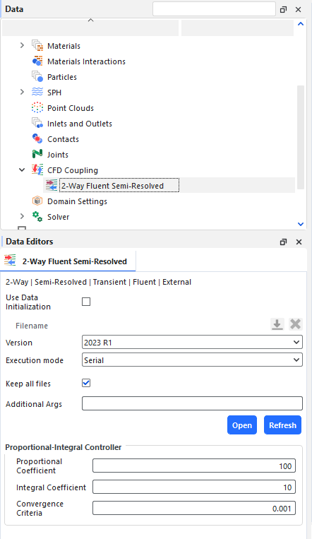
Table 1: 2-Way Fluent Semi-Resolved Settings
Setting | Description | Range |
|---|---|---|
Use Data Initialization | When selected, enables you to begin your simulation with an initial flow field based upon the Fluent fluid phases. This initial solution is saved from Fluent into a DAT (DAT.H5 or DAT.GZ) file that is then used by Rocky during processing. | Turns on or off |
Version | Enables you to select the Ansys Fluent software version you want to use for processing. Tip: If you do not see the Ansys version you expected, see also Rocky does not list my Ansys version when I try to set up 2-Way Fluent Coupling. | List automatically generated based upon the software versions detected. |
Execution mode | Enables you to select how your computer and/or network will process the fluid portion of the coupled simulation. Note: Regardless of what is selected here, the Rocky portion of the coupled simulation will still be processed according to the Simulation Target and related information that you specified on Solver General Settings tab (see also About Starting a Simulation. Specifically:
| Serial; Local Parallel; Distributed Parallel |
Solver Processes | When Local Parallel is selected for Execution mode, this enables you to determine the number of computer processors (threads) you want dedicated to the CFD solver. Note: You select the number of processors used by Rocky when you start processing the simulation. (See also About Starting a Simulation). Note: This text field does not support parametric variables. (See also I cannot enter an input variable or mathematical function into a text field). | Positive values |
Host Name | When Distributed Parallel is selected for Execution mode, this is the name of the remote machine on your network. Tip:Contact your IT administrator to find out the host names of the fluid nodes on your network. | 99 character limit |
Amount | When Distributed Parallel is selected for Execution mode, for each separate Host Name listed, this is the number of computer processors you want dedicated to the CFD solver. | Positive values |
Keep all files | When selected, all Fluent .dat files (and in some cases, as with moving meshes, .cas files as well) will be saved. When cleared, this enables you to select how many .dat (and sometimes .cas) Files to keep. Keeping fewer than all .dat (and sometimes .cas) files can help you save storage space when processing your simulation. However, doing so can also limit your fluid post-processing abilities, as well as your ability to restart the simulation from an earlier time due to the reduced amount of past fluid data that is available when you save fewer .dat (and sometimes .cas) files. | Turns on or off |
Files to keep | When Keep all files is cleared, this determines how many Fluent .dat files (and in some cases, as with moving meshes, .cas files as well) are saved. For example, if set to 1, only the last .dat (and sometimes .cas) files will be kept. If set to 2, only the last 2 .dat (and sometimes .cas) files will be kept, and so on. This setting can be useful in cases where you need only to keep files past steady state, for example, or when you do not require the Fluent files for post-processing. Important: If you decide to save fewer than all of the files, the number of .dat (and sometimes .cas) files you save will be as far back in time as you can restart your simulation since fluid data will not be available for prior times. Note: This text field does not support parametric variables. (See also I cannot enter an input variable or mathematical function into a text field). | Whole values greater than or equal to 1 |
Additional Args | This displays the set of arguments that Rocky passed "as-is" from the Fluent command line when the coupled simulation began. For advanced users, this enables more control of the Fluent portion of the processing. For more information about these arguments, see your Ansys Fluent documentation. | Positive values |
What would you like to do?
Exchange (2-Way) Rocky Particle Data with Semi-Resolved Fluid Flow Data from Ansys Fluent, which covers only the final coupling portion of the entire 2-Way Fluent Coupling procedure.
Use the 2-Way Fluent Semi-Resolved Method to Process a Fluent and Rocky Simulation, which covers the full procedure, including the setup steps that are required in Fluent.
See Also
Tip: This procedure covers only the final coupling portion of the entire 2-Way Fluent Semi-Resolved Coupling procedure, which applies to both multiphase and single phase coupling methods. To see the full procedure, including the setup steps that are required in Fluent, refer instead to Use the 2-Way Fluent Semi-Resolved Method to Process a Fluent and Rocky Simulation.
Important: Ensure that you have a Rocky-supported version of Ansys Fluent installed upon the same machine that contains your Rocky program installation. (See also System Requirements.) Note: If you are not certain whether you have installed the Ansys Fluent Coupling Support component during your Rocky installation, first follow the Install Ansys Coupling Components procedure before beginning these steps.
From the Data panel, click CFD Coupling and then from the Data Editors panel, choose Fluent Semi-Resolved from the Coupling Mode list.
From the Select Fluent CAS file dialog, locate and select the CAS (CAS.H5 or CAS.GZ) file you previously generated in Fluent, and then click Open. Important: A mesh validation step will occur immediately after the CAS file import. This requires a valid Fluent license on the same machine upon which you are running the Rocky simulation. After successful import, a new 2-Way Fluent Semi-Resolved item appears beneath CFD Coupling in the Data panel. In addition, if you chose to set up Moving Meshes in Fluent, one new Frame will appear under Motion Frames in the Data panel for each Cell Zone with motions you have defined. Important: If you have defined your Moving Meshes in Fluent using expressions, Rocky will not be able to create the associated Motion Frames for you automatically. Rather, you must manually create your own Motion Frames in Rocky to match the Fluent motions as closely as possible.
If the CAS (CAS.H5 or CAS.GZ) file imported new Motion Frames, assign each newly imported Frame to the geometry component you want to share corresponding movements with Fluent. (See also Apply a Motion Frame to an Imported Geometry.)
From the Data panel under CFD Coupling, select the new 2-Way Fluent Semi-Resolved item and then from the Data Editors panel, do all of the following:
Choose what fluid flow data Rocky starts with by doing one of the following:
To start your Rocky simulation without providing initial fluid flow data, ensure the Use Data Initialization checkbox remains cleared. Doing so ensures that the initialization settings prescribed in Fluent will be used to generate the initial fluid flow.
To start your Rocky simulation with initial fluid flow data, select Use Data Initialization, click the Import File button, and then select and open the DAT (DAT.H5 or DAT.GZ) file you want.
From the Version list, select what Ansys version you want to use for fluid coupling. Tip:If you do not see the Ansys version you expected, see also Rocky does not list my Ansys version when I try to set up 2-Way Fluent Coupling.
Choose how the fluid portion of the simulation is processed by doing one of the following:
To have it processed on only one processor on your local machine, from the Execution mode list, select Serial.
To have it processed on multiple processors on your local machine, from the Execution mode list, select Local Parallel and then from the Solver Processes field, enter the number of processors you want to dedicate to the CFD solver.
To have it processed across several machines on your network, from the Execution mode list, select Distributed Parallel and then do one of the following:
Under Hosts, click the Add button for each server you want to add and then for each row, define the Host name and Amount information.
To import an external list of hosts and amounts that you created outside of Rocky, click the Import File button, and then from the Import dialog, locate and select the TXT file containing the information, and then click Open. The Host section is populated with the information from the TXT file. Tip:The format for the TXT file needs to include the Host name repeated on separate lines for each Amount you want devoted. To see an example, create a few sample rows as specified directly above, click Export File and then save and view the results as a TXT file.
Choose how many Fluent files to keep by doing one of the following:
To keep each Fluent DAT (DAT.H5 or DAT.GZ) file (and in some cases, as with moving meshes, CAS files as well), enable the Keep all files checkbox. Important: Unless you require all files for post-processing in Fluent, keeping all files is not recommended for the 2-Way Fluent Semi-Resolved method. (See also About Using the 2-Way Fluent Semi-Resolved Method.)
To keep only the last (or last several) Fluent DAT (DAT.H5 or DAT.GZ) (and sometimes CAS) files saved, ensure the Keep all files checkbox is cleared, and then enter the number of last-saved files you want to keep in the Files to keep box. Tip:Keeping the last 2 (or more) files is recommended. Important: If you decide to save fewer than all of the files, be aware that you will not be able to post-process the unsaved files in Fluent. Also, be aware that the number of DAT (and sometimes CAS) files you save will be as far back in time as you can restart your simulation since fluid data will not be available for prior times. Tip:You can also choose which quantities and frequency you want to write to disk using Fluent's Autosave functionality.
Tips:
To verify or change the CAS (CAS.H5 or CAS.GZ) file selected, click Open and Rocky will open its own copy of the CAS (CAS.H5 or CAS.GZ) file in Fluent. From here, you can view or make changes to the Rocky copy of the file. Important: Because Rocky uses only its own copy of the imported CAS (CAS.H5 or CAS.GZ) file, it is critical that you only open the imported CAS (CAS.H5 or CAS.GZ) from Rocky's Open button, and that you save any changes to the default location Rocky indicates.
If you make changes to the Rocky copy of the CAS (CAS.H5 or CAS.GZ) file in Fluent, click Refresh to have Rocky include the updates. Important: The Refresh button works only if you first opened the CAS (CAS.H5 or CAS.GZ) file from the Rocky Open button.
If you made changes to your original Fluent version of the CAS (CAS.H5 or CAS.GZ) file and did not use the Rocky Open button as specified above, you must set the CFD Coupling option to No Coupling to clear the values, and then restart this procedure again from the beginning, selecting the updated CAS (CAS.H5 or CAS.GZ) file in step 3.
See Also:
If your Rocky project was opened through Workbench, an External Coupling component automatically appears in the Rocky Data panel. For Rocky projects coupled with Ansys Mechanical through Workbench, this component enables you to define the kind of data gets shared between the programs, such as the geometry loads.
For Rocky projects that are coupled with other Ansys products (not including Mechanical) through Workbench, this component can be ignored.
What would you like to do?
See Also:
If you have an External Coupling component in your Rocky Data panel, this indicates that your Rocky project has been opened through Workbench. Although it will appear for any type of coupled project that you open through Workbench, it is designed to work only with Rocky projects that are coupled specifically with Ansys Mechanical.
Tip: As a best practice, it is important to open workbench, insert the Rocky and Mechanical components (left figure below showing unattached Rocky and Transient Thermal), then manually open an save Rocky's project, and only then manually link Rocky to Mechanical (right figure below showing Rocky and Transient Thermal attached).
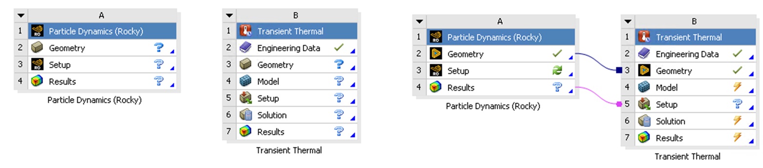
For projects coupled with Mechanical, defining the options for this component enables you to determine what kind of particle data to share, as described below.
For all other coupled projects, including those with only SpaceClaim or with only 1-Way Fluent, this External Coupling component can be ignored.
When you define options for the Geometry Loads component, you choose the geometry component(s) for which you want to share particle load data with the coupled Ansys Mechanical program, and the simulation time frame during which you want data (Figure 1).
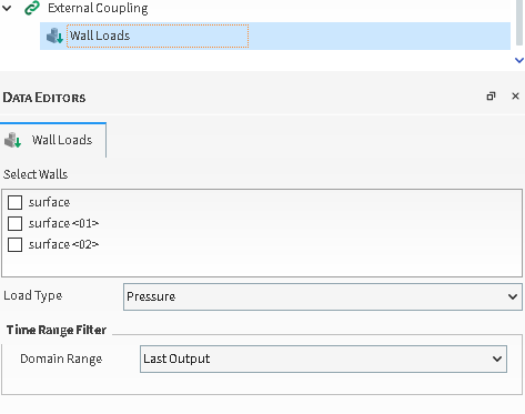
By limiting the data you share to only what you require for your analyses, you reduce the amount of time the coupled simulation will take to process.
Use the image above and table below to help you understand how to define options for Geometry Loads.
Table 1: Geometry Loads Parameter Definitions
Setting | Description | Range |
|---|---|---|
Select Geometries | Enables you to choose which geometry data will be shared during the coupled simulation. | Turns on or off |
Domain Range | Defines what timesteps of the simulation are included in the data to be shared. The options are as follows:
| Application Time Filter; All; Last Output; Time Range; Specify Time; After Time; Time Range Relative to Simulation End |
Initial | When Time Range or After Time is chosen for Domain Range, this is the starting time to begin the Timestep selection. | Any value between 0 and the final simulation time. |
Final | When Time Range is chosen for Domain Range, this is the ending time to stop the Timestep selection. | Any value between the Initial time and the final simulation time. |
At Time | When Specific Time is chosen for Domain Range, this is the exact moment in which the Timestep will be selected. | Any value between 0 and the final simulation time. |
Range from end | When Time Range Relative to Simulation End is chosen for Domain Range, this is the period of time before the final simulation time in which timesteps will be included in the selection. For example, when you want to include only the last X seconds of the simulation. | Any value between 0 and the final simulation time. |
What would you like to do?
See Also:
Note: Even though the External Coupling component appears for any type of Rocky project that is opened through Ansys Workbench, it only functions with projects that are coupled specifically with Ansys Mechanical.
Ensure that your Mechanical-coupled Rocky project has been opened through Workbench. (See also About Rocky and Ansys Workbench Integration.)
From the Data panel, under External Coupling, select Geometry Loads.
From the Data Editors panel, under Select Geometries, enable the checkbox for each geometry component for which you want to share data with the coupled Mechanical program.
Under Time Range Filter, choose the Domain Range and related options that define the time range during which you want to share data for the geometry component(s) you selected.
See Also:
When you wish to automatically transfer Rocky's HTC calculations to Mechanical, when connecting the Rocky system to a Steady-State or a Transient Thermal using Workbench, it is necessary to activate the Thermal calculations in Rocky's Physics (Physics thermal tab when HTC transfer between Rocky and Mechanical via Workbench is used.)
Figure 3.247: Physics thermal tab when HTC transfer between Rocky and Mechanical via Workbench is used.
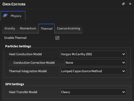
The module called SPH HTC Calculator should also be enabled:
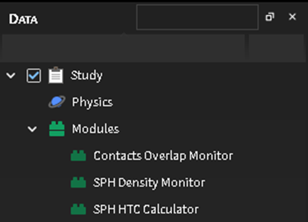
This enables another component in the External Coupling, the Heat Transfer Coefficient, which lets you assign the walls for which the HTC shall occur and the Time Range Filter for the transfer to happen:
Figure 3.249: Physics thermal tab when HTC transfer between Rocky and Mechanical via Workbench is used.
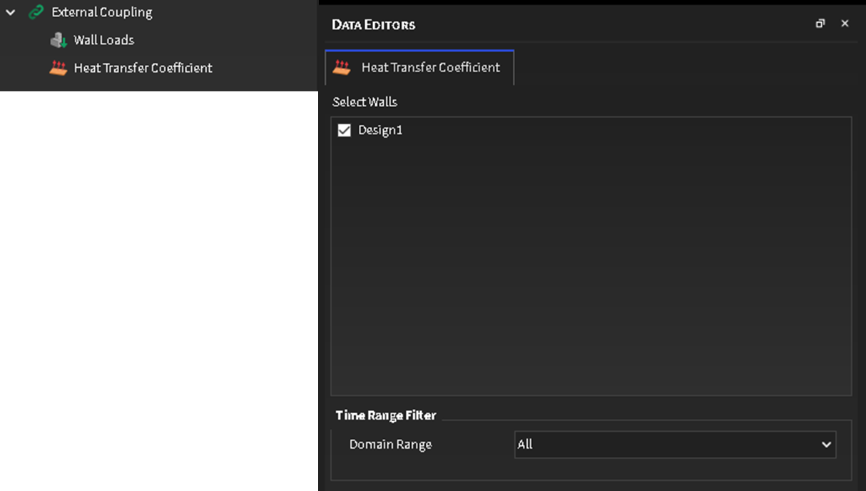
Use the image above and table below to help you understand how to define options for the HTC transfer.
Table 1: Heat Transfer Coefficient Parameter Definitions
|
Setting |
Description |
Range |
|---|---|---|
|
Select Walls |
Enables you to choose which geometry data will be shared during the coupled simulation. |
Turns on or off |
|
Time Range Filter |
Defines what timesteps of the simulation are included in the data to be shared. The options are as follows:
|
Application Time Filter; All; Last Output; Time Range; Specify Time; After Time; Time Range Relative to Simulation End |
|
Initial |
When Time Range or After Time is chosen for Domain Range, this is the starting time to begin the Timestep selection. |
Any value between 0 and the final simulation time. |
|
Final |
When Time Range is chosen for Domain Range, this is the ending time to stop the Timestep selection. |
Any value between the Initial time and the final simulation time. |
|
At Time |
When Specific Time is chosen for Domain Range, this is the exact moment in which the Timestep will be selected. |
Any value between 0 and the final simulation time. |
|
Range from end |
When Time Range Relative to Simulation End is chosen for Domain Range, this is the period of time before the final simulation time in which timesteps will be included in the selection. For example, when you want to include only the last X seconds of the simulation. |
Any value between 0 and the final simulation time. |
| Thermal Settings | Reference Temperature: defines the reference temperature for the HTC Calculation | Any value. |
What would you like to do?
See Also:
When you duplicate an item in the Data panel, you make an exact copy that you can then use as a starting place for making a similar but slightly different item, which can be quicker than starting from a brand new item.
You may duplicate many items in the Data panel including individual geometry components, individual material components, individual Particle sets, particle inputs, individual User Processes, and Motion Frames.
Ensure that the item you want to duplicate is already created and set up the way you want.
From the Data panel, right-click the item you want to copy, and then choose Duplicate. A copy of the item appears in the same list as the original item you chose, the name of which is appended with a new number.
See Also:
If you have the need to remove many separate items under the same Data panel category, you may remove all those items at one time with multi-select. These include many items in the Data panel such as individual geometry components, individual material components, individual Particle sets, particle inputs, and individual User Processes.
Under the Data panel category of your choice, use your mouse to multi-select all the individual components that you want to remove. Note: The multiple items must all belong to the same Data panel category.
Right-click the group of items you've selected, and then choose the Remove option. The items you selected will be removed from the list.
See Also: