


In Rocky, some data is collected automatically and some data you must first opt in to collecting before you process your simulation. In addition, some data is always collected right from the start of the simulation, and some data waits to be collected until passing certain thresholds that you define.
Use the topics below to help you understand what, how, and when data is collected in Rocky.
See Also:
Rocky provides many options for calculating, collecting, and analyzing different kinds of data.
Since calculating data you do not want can slow down your processing, and retaining data you do not need can take up valuable storage space, Rocky requires you to opt-in (or turn on) certain kinds of data collection. It does this to help you maximize your computing power and storage space.
To help you better understand how and when data is calculated, use the table below and the topics that follow.
Table 1: Rocky data and statistics collection matrix
|
Type of Data or Statistic |
How Collected |
When Collected |
See Also |
|---|---|---|---|
|
Affecting Geometries | |||
|
Surface wear modification |
Opt-in via the Use Wear checkbox (located on the Geometry | Wear tab) prior to processing. |
After Wear Start value is reached. |
Enable and View Surface Wear Modification on an Imported Geometry |
|
Collision effects on belts and boundaries as a result of particles interactions |
Opt-in via the Boundary Collisions Statistics Module prior to processing. |
Immediately |
Enable and View Collision Statistics for Boundaries |
|
Belt or boundary motions |
Automatic collection |
Immediately |
About Curves |
|
All other data related to geometries |
Automatic collection |
Immediately |
About Properties, About Curves |
|
Affecting Particles | |||
|
Particles energy spectra |
Enable the Particles Energy Spectra module prior to processing. |
After the module's Start Time value is reached. |
Enable and View Data for Particles Energy Spectra |
|
Particle breakage |
Automatic collection |
After Breakage Start value is reached. |
Enable and View Particle Breakage |
|
Fluid effects upon individual particles |
Opt-in via the CFD Coupling Particle Statistics Module prior to processing. |
After CFD Coupling Start Time value is reached |
Enable and View Fluid-Related Statistics for Particles |
|
Collision effects upon the surface of a Particle set |
Opt-in via the Intra-particle Collisions Statistics Module prior to processing. |
Immediately |
Enable and View Collision Statistics for Particle Surfaces (Intra) |
|
Collision effects upon each particle-particle and particle-boundary pair group within the simulation |
Opt-in via the Inter-group Collision Statistics Module prior to processing. |
Immediately |
Enable and View Inter-group Collision Statistics for Particles |
|
Collision effects upon individual particles resulting from interactions with other particles and boundaries |
Opt-in via the Inter-particle Collision Statistics Module prior to processing. |
Immediately |
Enable and View Collision Statistics for Particles Between Other Particles (Inter) |
|
Energy data for all Particle sets in the simulation |
Opt-in via the Particle Instantaneous Energies Module prior to processing. |
Immediately |
Enable and View Instantaneous Energies for Particles |
|
All other data related to particles |
Automatic collection |
Immediately |
About Properties, About Curves |
|
Affecting Contacts | |||
|
Contacts energy spectra |
Enable the Contacts Energy Spectra module prior to processing. |
After the module's Start Time value is reached. |
Enable and View Data for Contacts Energy Spectra |
|
Stress-related data (for analyzing via Eulerian Statistics User Process) |
Opt-in via the Collect Contacts Data checkbox on the Contacts entity prior to processing. |
Immediately |
Turn On Contacts Data Collection |
|
All other data related to Contacts |
Opt-in via the Collect Contacts Data checkbox on the Contacts entity prior to processing. |
Immediately |
Turn On Contacts Data Collection, About Contacts |
|
Affecting all other Rocky entities | |||
|
All other data related to all other entities |
Automatic collection |
Immediately |
About Properties, About Curves |
Note: If you have defined a Multiple Element (meshed) particle, what you have set for Meshed Particles Upscaling affects whether and how some post-processing properties and curves are displayed. (See also About Meshed Particles Upscaling.)
No matter how or when the data you want is collected, the resulting Properties (see also About Properties) can be visualized after processing in a view window and/or analyzed through a plot or histogram window. In addition, any resulting Curves (see also About Curves) can be analyzed through a plot or histogram window.
If you cannot see any of your simulation data and you know you have both collected it and have completed as much of the processing for which you want to have data, then you most likely have not yet created a view, plot, or histogram window by which to view and/or analyze the data or statistics you have collected.
Tip: Once your plot or histogram window is created (see also Graph Data within Rocky by Creating a Plot or Histogram), you can then modify the display to your liking (see also About Changing the Appearance of a Graph (Plot or Histogram)), export the data into a CSV file for further analysis outside of Rocky (see also Export Data into a CSV File), and more.
See Also:
In Rocky versions prior to 2022 R1, there was a built-in contact overlap monitor whose purpose was to check each contact pair (particle-particle or particle-boundary) for the amount that they overlapped, the percentage of which was determined by the size of the smallest particle in the contact pair.
During simulation processing, if at any timestep a contact pair's overlap exceeded one of three warning levels fixed at 2.5%, 10%, and 20%, a Contacts overlap message would be raised on the Simulation Log panel (Figure 1). (See also I get warnings or errors on my Simulation Log Panel.)
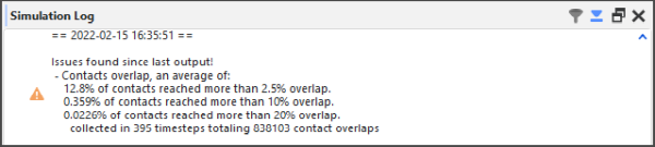
Monitoring your contacts for the size of their overlaps is important because Rocky is based on the soft-sphere approach, which uses the overlap value in order to compute collision forces. For example, in a typical simulation overlaps of 2.5% might be considered acceptable; however, simulations with overlaps larger than 10-20% should probably not be trusted as overlap values that large can lead to serious stability and accuracy issues.
Although it is a good practice to monitor overlap levels to guarantee they are below the desired values for a DEM solver, for some types of projects, the default warning levels Rocky uses might not be appropriate; or, it might be desired for there to be no overlap checks at all.
Therefore, as of Rocky 2022 R1, you are able to choose:
Whether or not you want contact overlaps to be monitored. Note: The monitor is "on" by default to match the behavior in older versions of Rocky.
What three overlap levels about which you want to be warned. Note: The initial values are set as to match the warning levels used in older versions of Rocky.
These tasks are accomplished via an embedded Module called Contacts Overlap Monitor (Figure 2).
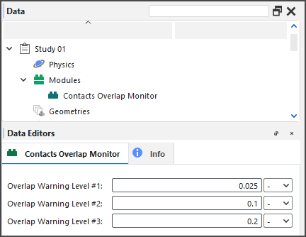 Figure 2: Options in the Data Editors
panel for the Contacts Overlap Monitor Module
Figure 2: Options in the Data Editors
panel for the Contacts Overlap Monitor Module
CONTACTS OVERLAP MONITOR OPTIONS
Use Figure 2 above and the table below to understand how to monitor your contact overlaps.
Table 1: Modules, Contacts Overlap Monitor parameter definitions
|
Setting |
Description |
Range |
|---|---|---|
|
Overlap Warning Level #1 |
Defines the value of the first (of three) overlap warning thresholds. If a contact pair's overlap-the percentage of which is based upon the size of the smallest particle in the contact pair-exceeds this value, a message will be raised on the Simulation Log panel. (See also About the Simulation Log Panel.) Note: The default value of 2.5% matches the built-in overlap used in prior versions of Rocky. |
Any value |
|
Overlap Warning Level #2 |
Defines the value of the second (of three) overlap thresholds. If a contact pair's overlap-the percentage of which is based upon the size of the smallest particle in the contact pair-exceeds this value, a warning will be raised on the Simulation Log panel. (See also About the Simulation Log Panel.) Note: The default value of 10% matches the built-in overlap used in prior versions of Rocky. |
Any value |
|
Overlap Warning Level #3 |
Defines the value of the third (of three) overlap thresholds. If a contact pair's overlap-the percentage of which is based upon the size of the smallest particle in the contact pair-exceeds this value, a warning will be raised on the Simulation Log panel. (See also About the Simulation Log Panel.) Note: The default value of 20% matches the built-in overlap used in prior versions of Rocky. |
Any value |
What would you like to do next?
The Contacts Overlap Monitor module is "on" (enabled) by default to match the behavior in older versions of Rocky.
Although it is a good practice to monitor overlap levels to guarantee they are below the desired values for a DEM solver, use the following procedure if you do not want to monitor contact overlaps in your simulation.
Note: This process can only be completed prior to processing your simulation.
To Turn Off the Overlap Monitor:
From the Data panel, select Modules.
From the Data Editors panel, clear the Contacts Overlap Monitor checkbox.
See Also:
CHANGE THE OVERLAP MONITOR WARNING LEVELS
The initial values defined in the Contacts Overlap Monitor module are designed to match the warning levels used in older versions of Rocky. Use the following procedure if you want to define different warning thresholds for your contact overlaps.
Note: This process can only be completed prior to processing your simulation.
To Change the Warning Level Values used in the Overlap Monitor:
From the Data panel, under Modules, select the Contacts Overlap Monitor entity.
From the Data Editors panel, enter the values you want for the three separate Overlap Warning Level fields.
See Also:
In Rocky, some boundaries data is collected automatically and some data you must first opt in to collecting before you process your simulation. In addition, some boundaries data is always collected right from the start of the simulation, and some data waits to be collected until passing certain thresholds that you define.
Use the topics below to help you understand what, how, and when boundaries data is collected in Rocky.
COLLISION STATISTICS FOR BOUNDARIES
By default, Rocky automatically collects data about the surface, make-up, and movement of individual geometries and conveyors. However, if you want to analyze the effects of particles colliding with these boundaries (for example, to study collision frequency, intensities, impact velocities, and so on), you will need to turn on Boundary Collision Statistics collection prior to processing your simulation.
About Collecting Boundary Collision Statistics
If you want to analyze this type of information in your simulation, you must first enable its collection via its module prior to processing your simulation.
Because collecting collisions statistics can take more processing time, memory, and disk storage due to increased file sizes, Rocky enables you to select from one or more sub-categories of statistics to collect. These are made available through the Boundary Collisions Statistic Module (Figure 1).
Figure 2.167: Options in the Data Editors panel when the Boundary Collision Statistics Module is enabled
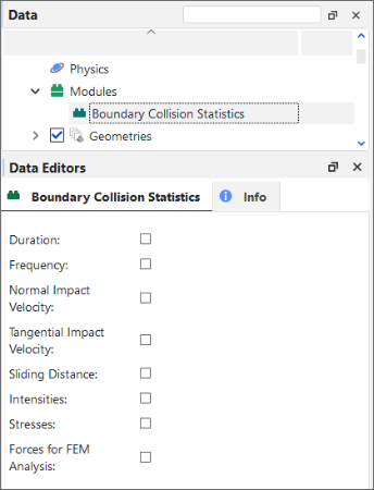
Tip: To maximize your processing capabilities, choose only the statistics that you require for your analyses.
During processing, Rocky collects the selected collision statistics between two consecutive output time levels for all boundaries in your project.
Tip: To view walk-through examples of collecting and analyzing boundary collisions statistics, refer to the following Tutorials:
About Analyzing Boundary Collision Statistics
Once the collisions data is collected (post-processing), specific collisions-related Properties (Figure 2) and Curves (Figure 3) will be available for the geometry or conveyor you select. (See also About Properties and About Curves.) The specific Properties and Curves available depends upon which statistics you enabled prior to processing.
Tip: These properties will be categorized as Statistical in the Evaluation column. (See also About Viewing an Individual Statistic.)
You can then choose to analyze the resulting Properties or Curves in a plot or histogram window. (See also Graphing (Plot or Histogram) a Data Set Within Rocky)
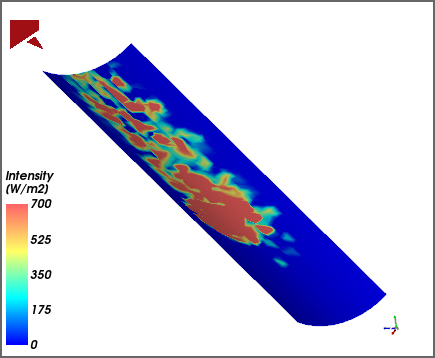
Or, you can then choose to display the Properties information graphically on the surface of your boundaries in a 3D View window. This can be useful, for example, for showing a color map of surface intensity (Figure 3). (See also View a Color Map of Wear on the Default Belt or Imported Geometry Itself.)
By using the Properties tab for the geometry, the options on the Coloring tab, and/or by using the slider on the Time toolbar (see also About the Time Toolbar), you can change how the data appears in the window. Tip: You may also limit your data further by using Time Statistics Properties. (See also About Adding and Editing Time Statistics Properties.)
Tip: Learn more by referring to the "Collision statistics" section in the DEM Technical Manual. (From the Rocky Help menu, point to Manuals, and then click DEM Technical Manual.)
Boundary Collision Statistics Collection Options
Use Figure 1 above and the table below to understand how to collect collision statistics for your boundaries.
Table 1: Modules, Boundary Collision Statistics parameter definitions
|
Setting |
Description |
Range |
|---|---|---|
|
Duration |
When enabled, Rocky will collect the mean, standard deviation, skewness, and kurtosis values of the duration of the collisions recorded in different regions of the geometry, during an interval between two consecutive output times. This can be useful when you are able to relate the duration to the amount of mass or heat transferred, for instance, in simulations involving chemical reactions and/or heat transfer. |
Turns on or off |
|
Forces for FEM Analysis |
When enabled, Rocky will collect the average force in various directions for each individual geometry node. This can be useful for analyzing directional forces, or side thrust. |
Turns on or off |
|
Frequency |
When enabled, Rocky will collect the average collision frequency recorded in different regions of the geometry, during an interval between two consecutive output times. This can be useful for analyzing shot flow, or for understanding the distribution of the frequency of the collisions against the surface triangles. |
Turns on or off |
|
Intensities |
When enabled, Rocky will collect the average dissipation and impact power values measured by each individual geometry triangle. This can be useful for analyzing impact wear or power draw. |
Turns on or off |
|
Normal Impact Velocity |
When enabled, Rocky will collect the mean, standard deviation, skewness, and kurtosis values of the impact relative velocity in the normal direction resulting from the collisions recorded in different regions of the geometry, during an interval between two consecutive output times. This can be useful for analyzing impact wear. |
Turns on or off |
|
Sliding Distance |
When enabled, Rocky will collect the mean, standard deviation, skewness, and kurtosis values of the sliding distance, which is the distance that a particle moves during a collision, parallel to the boundary triangle plane where the collision occurs. This can be useful for analyzing shear wear. |
Turns on or off |
|
Stresses |
When enabled, Rocky will collect the adhesion (if applicable; see note), normal and tangential stress values measured by each individual geometry triangle. This can be useful for analyzing the distribution of load due to particle collisions on a geometry. Note: Adhesive stresses are collected only when an Adhesive Force model (other than None) is enabled (see also About Physics Parameters), and an Adhesive Force Fraction for a boundary-boundary and/or boundary-particle Materials Interaction pair has a value set higher than zero (see also About Modifying Materials Interactions and Adhesion Values). |
Turns on or off |
|
Tangential Impact Velocity |
When enabled, Rocky will collect the mean, standard deviation, skewness, and kurtosis values of the impact relative velocity in the tangential direction resulting from the collisions recorded in different regions of the geometry, during an interval between two consecutive output times. This can be useful for analyzing impact wear. |
Turns on or off |
What would you like to do next?
Learn more about how to Add and Edit Geometry Components
Learn more About Collecting Data in Rocky
Enable and View Collision Statistics for Boundaries
Analyzing collision statistics for boundaries (see also About Collision Statistics for Boundaries) involves turning on the collection of the collision properties you want prior to processing your simulation.
After processing, you are then able to analyze the resulting Properties and/or Curves as you normally would.
To Enable and View Collision Statistics for Boundaries:
Set up the simulation as you normally would. (See also Set Simulation Parameters.)
Before processing your simulation, do all of the following:
From the Data panel, select Modules, and then from the Data Editors panel, select Boundary Collision Statistics.
From the Data panel, under Modules, select the new Boundary Collision Statistics entry.
From the Data Editors panel, select the checkboxes for the type of statistics you want collected. (See also About Collision Statistics for Boundaries.)
Verify that the default conveyor or imported geometry has its Triangle Size set small enough to enable the detail you want. (0.1 m is recommended for most chutes and mills). (From the Data panel under Geometry, select the component you want to verify. From the Data Editors panel, on the Geometry sub-tab, verify the Triangle Size value.)
Process the simulation as you normally would. (See also Processing a Simulation.)
From the Data panel, under Geometries, select the component that you want to analyze.
From the Data Editors panel, select either the Properties or the Curves tab.
Create a plot (see also Graph Data within Rocky by Creating a Plot or Histogram) or visualize the data in a 3D View window (see also About 3D View Windows). Tips:
With Properties, you can also choose to View a Color Map of Wear on the Default Belt or Imported Geometry Itself.
You may also limit your data further by using Time Statistics Properties. (See also About Adding and Editing Time Statistics Properties.)
See Also:
In Rocky, some Particles data is collected automatically and some data you must first opt in to collecting before you process your simulation. In addition, some Particles data is always collected right from the start of the simulation, and some data waits to be collected until passing certain thresholds that you define.
Use the topics below to help you understand what, how, and when Particles data is collected in Rocky.
ABOUT INTER-GROUP CCOLLISION STATISTICS
If you want to analyze the effects of collisions upon various particle-particle or particle-boundary pair groups within your simulation, you can choose to collect Inter-group Collision Statistics prior to processing your simulation.
About Collecting Inter-group Collision Statistics
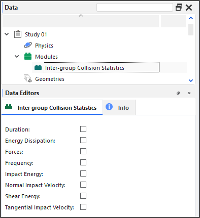
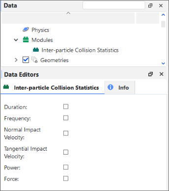
Because collecting collisions statistics can take more processing time, memory, and disk storage due to increased file sizes, Rocky enables you to select from one or more sub-categories of statistics to collect. These are made available through the Inter-group Collision Statistics Module (Figure 1).
Figure 2.171: Options in the Data Editors panel when the Inter-group Collision Statistics Module is enabled
In addition, only particles and geometries belonging to particle groups and geometry components that have been enabled for Inter-group Collision Statistics collection will be recorded (Figures 2 and 3).
Figure 2.172: Additional module options for Particle groups when the Inter-group Collision Statistics module is enabled
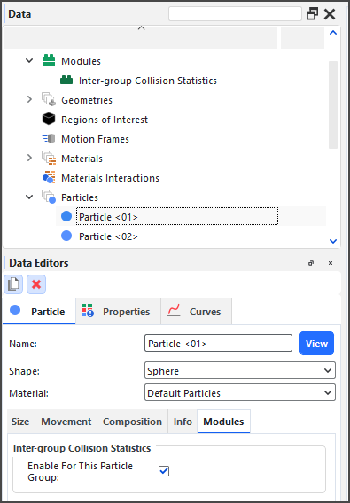
Figure 2.173: Additional module options for a geometry component when the Inter-group Collision Statistics module is enabled
Tip: To maximize your processing capabilities, choose only the statistics that you require for your analyses.
During processing, Rocky collects the selected collision statistics between two consecutive output time levels for each participating particle-particle and particle-boundary pair.
About Analyzing Inter-group Collision Statistics
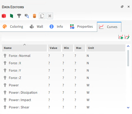
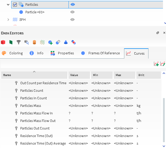
Once the collisions data is collected (post-processing), specific collisions-related Curves (Figure 2) will be available for the main Particles entity. (See also About Curves.)
Figure 2.174: Curves for Particles (simulation-wide) when Inter-group Collision Statistics are enabled
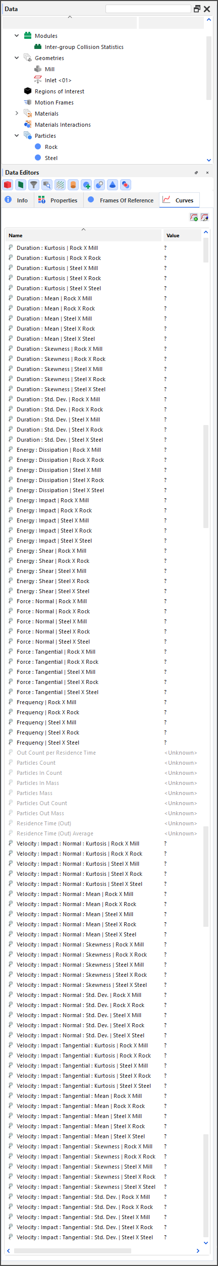
Note: For all Inter-group Collisions Statistics curves, the effects of upscaling will be ignored for any meshed particles with Meshed Particles Upscaling enabled. (See also About Meshed Particles Upscaling.)
You can then choose to analyze the resulting Curves in a time or cross plot window. (See also Graphing (Plot or Histogram) a Data Set Within Rocky.)
Tip: Learn more by referring to the "Collision statistics" section in the DEM Technical Manual. (From the Rocky Help menu, point to Manuals, and then click DEM Technical Manual.)
Inter-group Collision Statistics Collection Options
Use Figure 1 above and the table below to understand how to collect Inter-group Collision Statistics.
Table 1: Modules, Inter-group Collision Statistics parameter definitions
|
Setting |
Description |
Range |
|---|---|---|
|
Duration |
When enabled, Rocky will collect the mean, standard deviation, skewness, and kurtosis values of the duration of the collisions recorded for each particle-particle and particle-boundary pair in the simulation. |
Turns on or off |
|
Energy Dissipation |
When enabled, Rocky will collect the energy dissipation values of the collisions recorded for each particle-particle and particle-boundary pair in the simulation. |
Turns on or off |
|
Forces |
When enabled, Rocky will collect the average force in both the normal and tangential directions of the collisions recorded for each particle-particle and particle-boundary pair in the simulation. |
Turns on or off |
|
Frequency |
When enabled, Rocky will collect the average frequency of the collisions recorded for each particle-particle and particle-boundary pair in the simulation. |
Turns on or off |
|
Impact Energy |
When enabled, Rocky will collect impact energy values of the collisions recorded for each particle-particle and particle-boundary pair in the simulation. |
Turns on or off |
|
Normal Impact Velocity |
When enabled, Rocky will collect the mean, standard deviation, skewness, and kurtosis values of the impact relative velocity in the normal direction of the collisions recorded for each particle-particle and particle-boundary pair in the simulation. |
Turns on or off |
|
Shear Energy |
When enabled, Rocky will collect shear energy values of the collisions recorded for each particle-particle and particle-boundary pair in the simulation. |
Turns on or off |
|
Tangential Impact Velocity |
When enabled, Rocky will collect the mean, standard deviation, skewness, and kurtosis values of the impact relative velocity in the tangential direction of the collisions recorded for each particle-particle and particle-boundary pair in the simulation. |
Turns on or off |
What would you like to do next?
See Also:
ABOUT INTRA-PARTICLE COLLISION STATISTICS
For certain solid and flexible Particle sets in Rocky (see Supported Particle Sets section below), you can choose to have collision data between two consecutive output time levels collected by Rocky during the simulation. In this version of Rocky, this is referred to as Intra-particle Collision Statistics.
About Collecting Intra-particle Collision Statistics
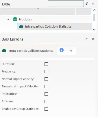
Because collecting collisions statistics can take more processing time, memory, and disk storage due to increased file sizes, Rocky enables you to select from one or more sub-categories of statistics to collect. These are made available through the Intra-particle Collision Statistics Module (Figure 1).
Figure 2.175: Options in the Data Editors panel when the Intra-particle Collision Statistics Module is enabled
Tip: To maximize your processing capabilities, choose only the statistics that you require for your analyses.
During processing, Rocky collects the selected collision statistics between two consecutive output time levels for all applicable particle sets in your project.
Tip: To see a walk-through example of collecting and analyzing Intra-particle collisions statistics, refer to Tutorial - Tablet Coater in the Rocky Tutorial Guide.
This feature works only with Particle sets that have the following characteristics:
Single size (or monosized) only. (No particle size distributions (PSDs).)
Unbroken shapes only. (No breakage modeling.)
For Solids, Polyhedron or Custom Polyhedrons (either concave or convex) shapes only; can be either rigid or flexible, however. (No Spheres nor any type of Sphero-shapes; no Briquettes nor Faceted Cylinder shapes.)
For Fibers, flexible shapes only. (No single-element Fiber compositions. No Shell shapes of any kind, neither rigid nor flexible.)
(See also About Adding and Editing Particle Sets.)
Note: When used with Multi-Element (meshed) particles with Meshed Particles Upscaling enabled, Intra-particle Collision Statistics properties will be provided but the effects of upscaling will be ignored. This means that rather than providing data for the whole particle, data will be provided for each individual Element. (See also About Meshed Particles Upscaling.)
If you choose to enable Intra-particle Collision Statistics, then you must have at least one Particle set in your simulation that meets the above criteria. Otherwise, Rocky will not process the simulation, and you might see the following error:
Figure 2.176: Rocky error shown if no particle sets in the simulation support Intra-particle Collisions Statistics
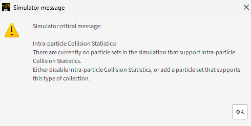
If you see this error after attempting to process your simulation, either disable Intra-particle Collision Statistics, or add a particle set that supports this type of collection.
About Analyzing Intra-particle Collisions Statistics
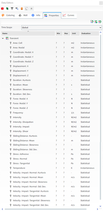
Once the collisions data is collected (post-processing), specific collisions-related Properties (Figure 3) will be available for the supported particle set you select. (See also About Properties.) The specific Properties available depends upon which statistics you enabled prior to processing.
Figure 2.177: Particles Details window showing Stress Normal collision statistics for a particle set
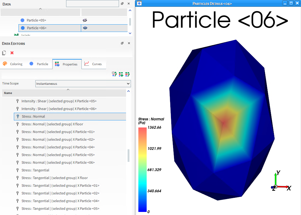
Tip: These properties will be categorized as Statistical in the Evaluation column. (See also About Viewing an Individual Statistic.)
Tip: Although it is possible to visualize the data at any time during processing, it is recommended that you avoid analyzing the data until the simulation reaches the point during which the particles are nearly constant (steady state). This is because the resulting data will have little meaning if the number of particles has a lot of variation.
You can then choose to display the collisions data graphically on the surface of a representative particle in the Particles Details window (Figure 3).
By using the slider on the Time toolbar (see also About the Time Toolbar), you can see how the data changes at different points in time.
Note: Because the Thermal Model considers a uniform temperature per individual particle, collision statistics cannot account for temperature. As a result, the Temperature property will not be available to view in a Particles Details window. However, in Collisions Statistics simulations that have both the Thermal Model enabled and use thermal-supported shape types (see also Particle and Input Limitations), you can still view the Temperature property from the main Particles entity, or from a 3D View window. (See also Enable Thermal Modeling Calculations.)
About Collision Statistics Visualization
In the collision statistics visualization, a value displayed at a given vertex is
representative of all collisions in the region of influence of the vertex that occurred in all
enabled particles of the particle set being analyzed, during the time lapse between two output
time levels. This means that data displayed at time  is the result of the statistics of the collision that happened between time
 and
and  , where
  is the output period.
As usual in these type of representations, values displayed at other, non-vertex points of the particle are obtained by interpolation of available values from the surrounding vertices.
In order to get a statistical value per particle, the collision statistics that happened during that output is divided by the number of enabled particles at the time when the statistics are displayed. Therefore, it is important that these statistics should be used only when you have reached a point during the simulation where the number of particles during that output is nearly constant.
Otherwise, for example, suppose you have 100 particles from the beginning of the output period to the middle of it, and at the last time step of the output period, you have only 1 particle. The statistics of all 100 particles that were there will be divided by 1 (the number of particles at the final time step of that output period), giving values much higher than expected.
Conversely, if you get these statistics at the beginning of your simulation and particles are entering, for example, you may have 0 particles at the beginning of the first output period and 1000 particles at the end. In this case, the collision statistics will be divided by 100 and will give values much smaller than expected.
Tip: Learn more by referring to the "Collision statistics" section in the DEM Technical Manual. (From the Rocky Help menu, point to Manuals, and then click DEM Technical Manual.)
Tip: To see a walk-through example of gathering and displaying collision statistics for particles, review Tutorial - Tablet Coater in the Rocky Tutorial Guide.
Intra-particle Collision Statistics Collection Options
Use Figure 1 above, and the figure and table below to understand how to collect Intra-particle Collisions Statistics.
Table 1: Modules, Intra-particle Collisions Statistics parameter definitions
|
Setting |
Description |
Range |
|---|---|---|
|
Duration |
When enabled, Rocky will collect the mean, standard deviation, skewness, and kurtosis values of the duration of the collisions recorded in different regions of the representative particle of the selected particle set, during an interval between two consecutive output times. This can be useful when you are able to relate the duration to a certain process, such as in simulations involving chemical reactions and/or heat transfer. |
Turns on or off |
|
Frequency |
When enabled, Rocky will collect the average collision frequency recorded in different regions of the representative particle of the selected particle set, during an interval between two consecutive output times. This can be useful for analyzing the distribution of the frequency of the collisions around the particle surface. |
Turns on or off |
|
Intensities |
When enabled, Rocky will collect the power transferred per unit area in different regions of the representative particle of the selected particle set. Specifically:
This can be useful for evaluating the impact work around the particle, perhaps to help avoid exaggerated wear in a certain region of the particle, for example. |
Turns on or off |
|
Normal Impact Velocity |
When enabled, Rocky will collect the mean, standard deviation, skewness, and kurtosis values of the impact relative velocity in the normal direction resulting from the collisions recorded in different regions of the representative particle of the selected particle set, during an interval between two consecutive output times. This can be useful when analyzing particle breakage or granules de-agglomeration, for example. |
Turns on or off |
|
Stresses |
When enabled, Rocky will collect the adhesion (if applicable; see note), normal and tangential stress values measured by different regions of the representative particle of the selected particle set. This can be useful for analyzing damage to the particle surface due the action of concentrated forces in certain regions. Note: Adhesive stresses are collected only when an Adhesive Force model (other than None) is enabled (see also About Physics Parameters), and an Adhesive Force Fraction for a particle-boundary and/or particle-particle Materials Interaction pair has a value set higher than zero (see also About Modifying Materials Interactions and Adhesion Values). |
Turns on or off |
|
Tangential Impact Velocity |
When enabled, Rocky will collect the mean, standard deviation, skewness, and kurtosis values of the impact relative velocity in the tangential direction resulting from the collisions recorded in different regions of the representative particle of the selected particle set, during an interval between two consecutive output times. This can be useful when analyzing particle breakage or granules de-agglomeration, for example. |
Turns on or off |
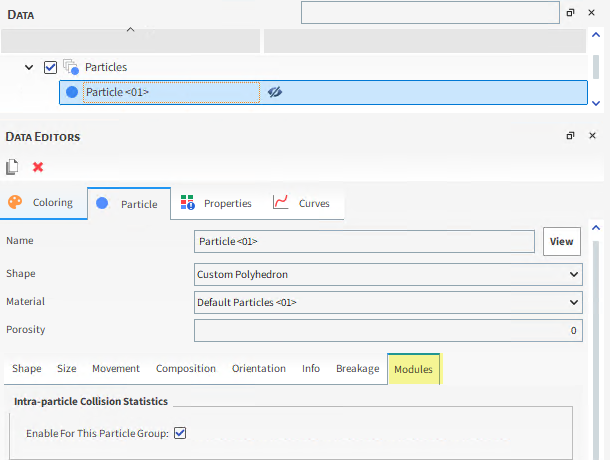
| Enable per Group Statistics | When enabled, Rocky will collect all the selected intra-particle statistics (from
Duration, Frequency, Normal Impact Velocity, Tangential Impact Velocity, Intensities
and Stresses) organized per group. This can be useful for analyzing how different
particle sets interact to the one being analyzed. In other words, it enables analyzing
the contribution of each particle group for the intra-particle collected statistics. Note: When enabled, a new Modules sub-tab is added to the main Particle tab on the Data Editors when a particle set is selected in the Data panel, as shown in Figure 2.178: Particle | Modules sub-tab available when Enable per Group Statistics is selected. In this sub-tab, you can enable or disable the intra-particle statistics collection for the specific particle group you are setting up by marking or clearing the Enable For This Particle Group checkbox, respectively.
|
Turns on or off |
What would you like to do next?
ABOUT INTER-PARTICLE COLLISION STATISTICS
If you want to expand the set of particle properties available for post-processing, including several statistical properties that may be collected during a simulation, you can choose to collect Inter-particle Collision Statistics prior to processing your simulation.
These can be useful when you need to extract data considering all collisions that happened to a certain particle between two output periods. For example, with impact velocity, you could relate that data to the chances of the particle breaking or causing it to de-agglomerate. With duration, you could relate that data to a certain mass or heat transfer process, or to a certain chemical reaction.
About Collecting Inter-particle Collision Statistics
Because collecting collisions statistics can take more processing time, memory, and disk storage due to increased file sizes, Rocky enables you to select from one or more sub-categories of statistics to collect. These are made available through the Inter-particle Collision Statistics Module (Figure 1).
Figure 2.179: Options in the Data Editors panel when the Inter-particle Collision Statistics Module is enabled
Tip: To maximize your processing capabilities, choose only the statistics that you require for your analyses.
During processing, Rocky collects the selected collision statistics between two consecutive output time levels for all particles in your project.
Note: Some Inter-particle Collision Statistics properties will not be provided for Multi-Element (meshed) particles if the Meshed Particles Upscaling feature is enabled. (See also About Meshed Particles Upscaling.)
Tip: To see a walk-through example of collecting and analyzing Inter-particle collisions statistics, refer to Tutorial - Tablet Coater in the Rocky Tutorial Guide.
ABOUT ANALYZING INTER-PARTICLE COLLISION STATISTICS
Once the collisions data is collected (post-processing), specific collisions-related Properties (Figure 2) will be available for the main Particles entity. (See also About Properties.) The specific Properties available depends upon which statistics you enabled prior to processing.
Figure 2.180: Properties available for the main Particles entity when Inter-particle Collision Statistics is enabled
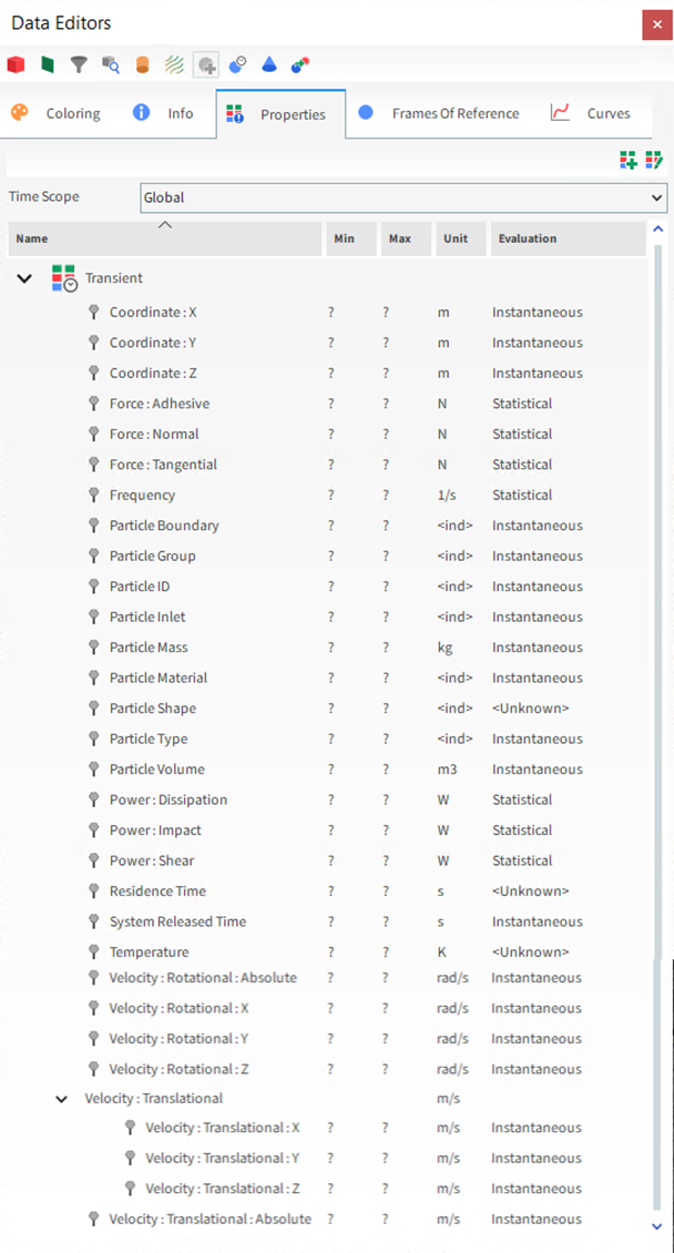
Tip: These properties will be categorized as Statistical in the Evaluation column. (See also About Viewing an Individual Statistic.)
You can then choose to analyze the resulting Properties in a plot or histogram window. (See also Graphing (Plot or Histogram) a Data Set Within Rocky.)
Or, you can choose to display the Properties information in a 3D View window. (See also About 3D View Windows.)
By using the Properties tab for the main Particles entity, the options on the Coloring tab, and/or by using the slider on the Time toolbar (see also About the Time Toolbar), you can change how the data appears in the window.
Tip: Learn more by referring to the "Collision statistics" section in the DEM Technical Manual. (From the Rocky Help menu, point to Manuals, and then click DEM Technical Manual.)
Inter-particle Collision Statistics Collection Options
Use Figure 1 above and the table below to understand how to collect Inter-particle Collision Statistics.
Table 1: Modules, Inter-particle Collision Statistics parameter definitions
|
Setting |
Description |
Range |
|---|---|---|
|
Duration |
When enabled, Rocky will collect the mean, standard deviation, skewness, and kurtosis values of the duration of the collisions recorded for each individual whole particle or fragment, during an output timestep. This can be useful when you are able to relate the duration to a certain process, such as in simulations involving chemical reactions and/or heat transfer. For example, when a homogeneous system is desired, you might seek similar collision durations across particles to help ensure a uniform distribution of the transferred quantity. Note: To make use of this property with Multi-Element (meshed) particles, the Meshed Particles Upscaling feature must be disabled. (See also About Meshed Particles Upscaling.) |
Turns on or off |
|
Force |
When enabled, Rocky will collect the sum of the forces in both the Normal and Tangential directions and for adhesion (if applicable; see note) as recorded for each individual whole particle or fragment. Note: Adhesive forces are collected only when an Adhesive Force model (other than None) is enabled (see also About Physics Parameters), and an Adhesive Force Fraction for a particle-boundary and/or particle-particle Materials Interaction pair has a value set higher than zero (see also About Modifying Materials Interactions and Adhesion Values). |
Turns on or off |
|
Frequency |
When enabled, Rocky will collect the average collision frequency recorded for each individual whole particle or fragment, during an output timestep. |
Turns on or off |
|
Normal Impact Velocity |
When enabled, Rocky will collect the mean, standard deviation, skewness, and kurtosis values of the impact relative velocity in the normal direction resulting from the collisions recorded for each individual whole particle or fragment, during an output timestep. Note: To make use of this property with Multi-Element (meshed) particles, the Meshed Particles Upscaling feature must be disabled. (See also About Meshed Particles Upscaling.) |
Turns on or off |
|
Power |
When enabled, Rocky will collect the dissipation and impact power values resulting from the collisions recorded for each individual whole particle or fragment, during an output timestep. |
Turns on or off |
|
Tangential Impact Velocity |
When enabled, Rocky will collect the mean, standard deviation, skewness, and kurtosis values of the impact relative velocity in the tangential direction resulting from the collisions recorded for each individual whole particle or fragment, during an output timestep. Note: To make use of this property with Multi-Element (meshed) particles, the Meshed Particles Upscaling feature must be disabled. (See also About Meshed Particles Upscaling.) |
Turns on or off |
What would you like to do next?
ABOUT FLUID-RELATED STATISTICS FOR PARTICLES
For most CFD Coupling options where the fluid flow affects the motion of the particles (1-Way Constant, 1-Way Fluent, and 2-Way Fluent), you can choose to collect CFD Coupling Particle Statistics prior to processing your simulation.
These can be useful when you need to extract data considering the fluid effects upon a particle between two output periods.
Important: The 2-Way Fluent Semi-Resolved method does not compute the forces individually. Therefore, when this module is enabled within a 2-Way Fluent Semi-Resolved case, it will not return the fluid forces.
About Collecting Fluid-Related Statistics for Particles
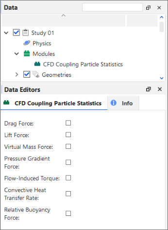
Because collecting statistics can take more processing time, memory, and disk storage due to increased file sizes, Rocky enables you to select from one or more sub-categories of statistics to collect. These are made available through the CFD Coupling Particle Statistics Module (Figure 1).
Figure 2.181: Options in the Data Editors panel when the CFD Coupling Particle Statistics Module is enabled
Tip: To maximize your processing capabilities, choose only the statistics that you require for your analyses.
During processing, Rocky collects the selected fluid-related statistics between two consecutive output time levels for all particles in your project.
About Analyzing Fluid-Related Statistics for Particles
Once the data is collected (post-processing), specific fluid-related Properties (Figure 2) will be available for the main Particles entity. (See also About Properties.) The specific Properties available depend upon which statistics you enabled prior to processing.
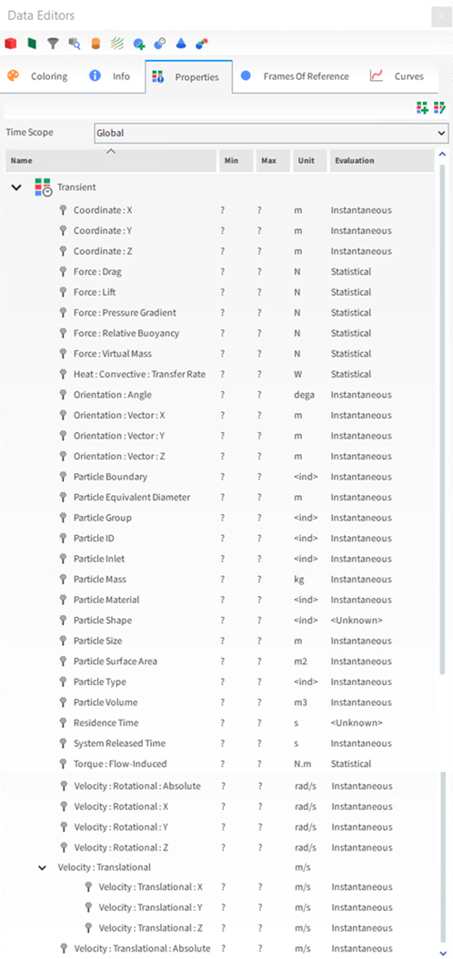 Figure 2: Properties available for the
main Particles entity when CFD Coupling Particle Statistics is enabled
Figure 2: Properties available for the
main Particles entity when CFD Coupling Particle Statistics is enabled
Tip: These properties will be categorized as Statistical in the Evaluation column. (See also About Viewing an Individual Statistic.)
You can then choose to analyze the resulting Properties in a plot or histogram window. (See also Graphing (Plot or Histogram) a Data Set Within Rocky.)
Or, you can choose to display the Properties information in a 3D View window. (See also About 3D View Windows.)
By using the Properties tab for the main Particles entity, the options on the Coloring tab, and/or by using the slider on the Time toolbar (see also About the Time Toolbar), you can change how the data appears in the window.
CFD Coupling Particle Statistics Collection Options
Use Figure 1 above and the table below to understand how to collect Fluid-Related Statistics for Particles.
Table 1: Modules, CFD Coupling Particle Statistics parameter definitions
|
Setting |
Description |
Range |
|---|---|---|
|
Convective Heat Transfer Rate |
When enabled, Rocky will collect the average convective heat transfer rate exchanged between a particle and the surrounding fluids as recorded for each individual whole particle or fragment. Note: Data is collected only when the Thermal Model is enabled and a Convective Heat Transfer Law has been defined for the fluid-particle interactions. |
Turns on or off |
|
Drag Force |
When enabled, Rocky will collect the average drag force applied by fluids as recorded for each individual whole particle or fragment. |
Turns on or off |
|
Flow-Induced Torque |
When enabled, Rocky will collect the average torque induced by fluid flow as recorded for each individual whole particle or fragment. Note: Data is collected only when a Torque Law has been defined for the fluid-particle interactions. |
Turns on or off |
|
Lift Force |
When enabled, Rocky will collect the average lift force applied by fluids as recorded for each individual whole particle or fragment. Note: Data is collected only when a Lift Law has been defined for the fluid-particle interactions. |
Turns on or off |
|
Pressure Gradient Force |
When enabled, Rocky will collect the average pressure gradient force applied by fluids as recorded for each individual whole particle or fragment. |
Turns on or off |
|
Virtual Mass Force |
When enabled, Rocky will collect the average virtual mass force applied by fluids as recorded for each individual whole particle or fragment. Note: Data is collected only when a Virual Mass Law has been defined for the fluid-particle interactions. |
Turns on or off |
What would you like to do next?
ABOUT PARTICLE INSTANTANEOUS ENERGIES
If you want to perform global or partial energy balances in a simulation, you can choose to collect particle instantaneous energies prior to processing your simulation, which enables the calculation of the kinetic and potential energies of each individual particle in the simulation.
About Collecting Particle Instantaneous Energies
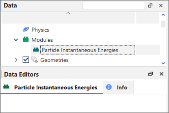
You choose to collect these kind of particle energies by enabling the Particle Instantaneous Energies Module (Figure 1).
Figure 2.182: There are no options in the Data Editors panel when the Particle Instantaneous Energies Module is enabled
During processing, Rocky collects particle energies data for each particle based upon its translational/rotational velocity and position in space.
About Analyzing Particle Instantaneous Energies
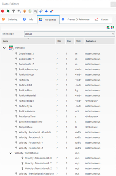
Once the energies data is collected (post-processing), specific energy-related Properties (Figure 2) and Curves (Figure 3) will be available for the main Particles entity. (See also About Properties and About Curves.)
Figure 2.183: Properties for Particles (simulation-wide) when Particle Instantaneous Energies is enabled
These Properties are based on the following energies calculations:
Translational kinetic energy: The energy related to the rectilinear motion of a particle. It is given by:
 where:
  is the particle's mass, and
  is the velocity of its center of mass.
 Rotational kinetic energy: This is the energy due to the rotation of a particle around an axis through its center of mass. It is given by:
 where:
  is the particle's angular velocity, and
  is the moment of inertia tensor.
 Potential energy: This is the energy of a particle due to its position relative to the Earth's gravitational field. In Rocky it is calculated as:
 where:
  is the particle's mass,
  is the acceleration due to gravity, and
  is the position vector of the particle's center of mass. Conventionally,
a zero potential energy is attributed to a plane orthogonal to the gravity direction,
passing through the origin of the coordinate system.
is the position vector of the particle's center of mass. Conventionally,
a zero potential energy is attributed to a plane orthogonal to the gravity direction,
passing through the origin of the coordinate system.
Figure 2.184: Curves for Particles (simulation-wide) when Particle Instantaneous Energies is enabled
The Energy Delta Curve represents a variation (delta) in total energy of the particles recorded during an interval between two consecutive output times.
You can choose to visualize the resulting Properties and Curves in a 3D View window (Figure 3), or analyze the results in a time or other plot window. (See also Graphing (Plot or Histogram) a Data Set Within Rocky.)
What would you like to do next?
See Also:
ENABLE AND VIEW INTER-GROUP COLLISION STATISTICS FOR PARTICLES
Analyzing Inter-group Collision Statistics for each particle-particle or particle-boundary pair group (see also About Inter-group Collision Statistics) involves turning on the collection of the collision properties you want prior to processing your simulation, and then determining which particle groups and geometries you want to involve in that collection.
After processing, you are then able to analyze the resulting Curves.
To Collect and View Inter-group Collision Statistics:
Set up the simulation as you normally would. (See also Set Simulation Parameters.)
Before processing your simulation, do all of the following:
From the Data panel, select Modules, and then from the Data Editors panel, select the Inter-group Collision Statistics checkbox.
From the Data panel, under Modules, select the new Inter-group Collision Statistics entry.
From the Data Editors panel, select the checkbox for each type of statistics you want collected. (See also About Inter-group Collision Statistics.)
For each geometry component that you do not want included in the collection of Inter-group Collision Statistics, do the following:
From the Data panel, under Geometries select the geometry that you want to exclude from Inter-group Collision Statistics collections.
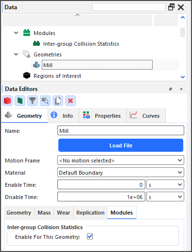
From the Data Editors panel, select the Geometry | Modules tab and then under Inter-group Collision Statistics clear the Enable For This Geometry checkbox.
For each particle group that you do not want included in the collection of Inter-group Collision Statistics, do the following:
From the Data panel, under Particles select the particle group that you want to exclude from Inter-group Collision Statistics collections.
From the Data Editors panel, select the Particle | Modules tab and then under Inter-group Collision Statistics clear the Enable For This Particle Group checkbox.
Process the simulation as you normally would. (See also Processing a Simulation.)
From the Data panel, select the main Particles entity.
From the Data Editors panel, select the Curves tab.
Create a time or cross plot. (See also Graph Data within Rocky by Creating a Plot or Histogram.)
See Also:
ENABLE AND VIEW COLLISION STATISTICS FOR PARTICLE SURFACES (INTRA)
Analyzing collision statistics for particle surfaces involves first turning on the collection of Intra-particle Collision Statistics prior to processing the simulation (see also About Intra-Particle Collision Statistics), and then viewing the resulting Properties for a supported Particle set on the surface of a representative particle in a Particles Details window.
By using the slider on the Time toolbar (see also About the Time Toolbar), you can see how the data changes at different points in time.
To Collect and View Collision Statistics for Particle Surfaces (Intra:
Set up your simulation as you normally would (see also Setting Up a Simulation). Note: If you decide to enable the Thermal Model, know that while the Temperature property will not be available to view on the Particles Details window, it can still be viewed from the main Particles entity or through a 3D View window. (See also Enable Thermal Modeling Calculations.)
Before processing your simulation, do all of the following:
From the Data panel, select Modules, and then from the Data Editors panel, select the Intra-particle Collision Statistics checkbox.
From the Data panel, under Modules, select the new Intra-particle Collision Statistics entity.
From the Data Editors panel, enable the checkboxes for the type of statistics you want collected. (See also About Intra-Particle Collision Statistics.)
Ensure you have added at least one Particle set that is eligible for intra-particle collision statistics collection. Note: Intra-particle collision statistics can be collected only on single sized particle sets that have no breakage enabled and that make use of the following shapes:
Polyhedron (rigid or flexible)
Custom Polyhedron (convex or concave, rigid or flexible)
Straight Fiber or Custom Fiber (flexible only)
(See also About Adding and Editing Particle Sets.)
Process your simulation as you normally would (see also About Starting a Simulation.)
From the Data panel, under Particles, select the Particle set for which you want to view intra-particle collision statistics, and then click the View button. A new Particles Details window opens showing a particle that represents the whole Particle set.
Display intra-particle collision statistics Properties on the view in one of the following ways:
From the Properties tab, click a Property and then drag and drop it on the Particles Details window. (See also About Properties.) Tips: You may also make use of Time Statistics Properties. (See also About Adding and Editing Time Statistics Properties.)
From the Coloring tab, use the Property lists to change what is colored in the Particles Details window. (See also Use the Coloring Tab to Change the Preview for a Particle Set.)
Use the slider on the Time toolbar to change what timestep is displaying data. (See also About the Time Toolbar.) Note: The data displayed at a given timestep was collected in the interval between that timestep and the previous one.
Tips:
Use your mouse to zoom, pan, and rotate the view, just as you would in a 3D View window. (See also Use the Mouse, Keyboard, or Toolbar to Change a 3D View.)
Change the look of the window by right-clicking the window, or by using the options on the Windows Editors panel. (See also About Using the Window Editors Panel to Change the Selected Particles Details Window.)
See Also:
ENABLE AND VIEW COLLISION STATISTICS FOR PARTICLES BETWEEN OTHER PARTOCLES (INTER)
Analyzing inter-particle collision statistics (see also About Inter-particle Collision Statistics) involves turning on the collection of the collision properties you want prior to processing your simulation.
After processing, you are then able to analyze the resulting Properties as you normally would.
To Collect and View Collision Statistics for Particles Between Other Particles (Inter:
Set up the simulation as you normally would. (See also Set Simulation Parameters.)
Before processing your simulation, do all of the following:
From the Data panel, select Modules, and then from the Data Editors panel, enable the Inter-particle Collision Statistics checkbox.
From the Data panel, under Modules, select the new Inter-particle Collision Statistics entry, and then from the Data Editors panel, enable the checkboxes for the type of statistics you want collected. (See also About Inter-particle Collision Statistics.)
Process the simulation as you normally would. (See also Processing a Simulation.)
From the Data panel, select the main Particles entity.
From the Data Editors panel, select the Properties tab.
Create a plot (see also Graph Data within Rocky by Creating a Plot or Histogram), or visualize the data in a 3D View window (see also About 3D View Windows).
See Also:
ENABLE AND VIEW INSTANTANEOUS ENERGIES FOR PARTICLES
Analyzing Particle Instantaneous Energies (see also About Particle Instantaneous Energies) involves turning on the collection of energies data prior to processing your simulation.
After processing, you are then able to analyze the resulting Properties as you normally would.
To Collect and View Inter-group Collision Statistics:
Set up the simulation as you normally would. (See also Set Simulation Parameters.)
Before processing your simulation, do all of the following:
From the Data panel, select Modules.
From the Data Editors panel, select the Particle Instantaneous Energies checkbox.
Process the simulation as you normally would. (See also Processing a Simulation.)
From the Data panel, select the main Particles entity.
From the Data Editors panel, select the Properties tab.
Create a 3D View (see also View Geometries, Particles, Points, and Fluids in 3D) or plot (see also Graph Data within Rocky by Creating a Plot or Histogram).
See Also:
ENABLE AND VIEW FLUID-RELATED STATISTICS FOR PARTICLES
Analyzing fluid-related statistics for particles (see also About Fluid-Related Statistics for Particles) involves turning on the collection of the fluid-related properties you want prior to processing your CFD Coupling simulation.
After processing, you are then able to analyze the resulting Properties for the main Particles entity as you normally would.
To Collect and View Fluid-Related Statistics for Particles
Set up your CFD Coupling simulation as you normally would. (See also Set Simulation Parameters.)
Before processing your simulation, do all of the following:
From the Data panel, select Modules, and then from the Data Editors panel, enable the CFD Coupling Particle Statistics checkbox.
From the Data panel, under Modules, select the new CFD Coupling Particle Statistics entry, and then from the Data Editors panel, enable the checkboxes for the type of statistics you want collected. (See also About Fluid-Related Statistics for Particles.)
Process the simulation as you normally would. (See also Processing a Simulation.)
From the Data panel, select the main Particles entity.
From the Data Editors panel, select the Properties tab.
Create a plot (see also Graph Data within Rocky by Creating a Plot or Histogram), or visualize the data in a 3D View window (see also About 3D View Windows).
See Also:
COLLECTING DATA ON CONTACTS AND ENERGY SPECTRA
In Rocky, contacts and energy spectra data is collected only if you first opt in to collecting them before you process your simulation. After choosing to collect it, contacts data is always collected right from the start of the simulation. However, data for energy spectra waits to be collected until passing certain thresholds that you define.
Depending on the source of the energy values considered, two types of energy spectra plots are available in Rocky: Contacts Energy Spectra and Particles Energy Spectra.
With Contacts Energy Spectra, the energy values are collected collision-wise during the simulation and the resulting data is categorized by the contact pair (particle group and/or geometry).
With Particles Energy Spectra the energy values collected during the simulation are related only to particles, and the resulting data is classified by size and particle group.
Based upon your energy analysis needs, you can use either or both types of energy spectra in your simulation.
Important: The energy scale in all energy spectra plots is logarithmic, so zero is not a valid value for the minimum energy, therefore for Contacts and Particles energy spectra the minimum energy values must be greater than zero.
Use the topics below to help you understand what, how, and when contacts and energy spectra data is collected in Rocky.
In Rocky, it is possible simulate the breakage behavior of particles. (See also Enable Particle Breakage Calculations.) However, simulations with breakage enabled can increase the computational cost, taking longer to process the simulation. With this in mind, Rocky has another feature you can use to analyze breakage: Contacts Energy Spectra.
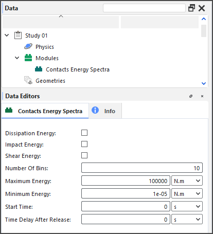
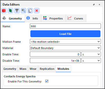
This useful tool collects different kinds of energy statistics per contact pair (particle group and/or geometry) and size, which helps provide insight into the distribution of the energies of all collisions that occurred in a simulation up to a given time. In this version of Rocky, these statistics are collected through the Contacts Energy Spectra module (Figure 1).
This kind of energy spectra is often used in conjunction with Particles Energy Spectra. (See also About Particles Energy Spectra.)
See the sections below for more information about this type of energy statistic, and how it is collected, calculated, and viewed in Rocky.
About Collecting Contact-Based Energy Statistics
For contact-based analysis, the energy statistics of particle collisions are collected per collision; i.e., every separate particle-to-particle or particle-to-geometry impact will have its resulting energy collision stored. Each statistics pair-which is composed of either two Particle sets or one Particle set and one Geometry-will present a separate Energy Spectra curve. In this version of Rocky, only particles and geometries belonging to particle groups and geometry components that have been enabled for energy spectra collection will be recorded (Figures 2 and 3).
Figure 2.187: Additional module options for Particle groups when the Contacts Energy Spectra module is enabled
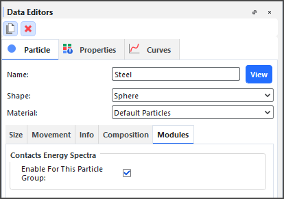
Figure 2.188: Additional module options for a geometry component when the Contacts Energy Spectra module is enabled
These curves are based upon three different types of collision energy, each of which can be useful for different types of analyses: Dissipation Energy, Impact Energy, and Shear Energy.
Because collecting statistics can take more processing time, memory, and disk storage due to increased file sizes, Rocky enables you to select which of these three collision energies you want to collect, and enables you to choose which particle groups and geometry components will participate in energy spectra collection.
About Setting Time Delays
It is important to realize that data is only collected after both the Start Time and Time Delay After Release values are reached. Data begins being collected at the Start Time but only for the particles that were released before the Time Delay After Release value. This is to allow enough time for the particle flow within your simulation to reach a steady state before the energy spectra calculations begin.
For example, if the Start Time is 5s, and the Time Delay After Release is 3s, a particle entering the simulation at 4s will only be accounted for after 7s of simulation time.
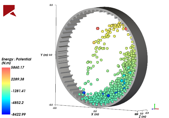
Applications for Contacts Energy Analysis
One common application of this type of analysis is for comminution devices like SAG mills (Figure 4), which use steel balls or other kinds of grinding media to help break rock or ore material into smaller fragments.
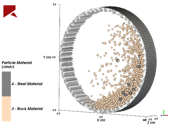
Although mills have great energy consumption, only a small part of this energy is converted into actual particle fragmentation. This inefficiency is mainly due to the fact that not all impacts lead to breakage. Impacts of low energy will not cause breakage, while excessive intensity impacts apply only part of the total energy to the breakage process. The rest of this energy is lost.
Therefore, it is important to understand how power is consumed during comminution processes in order to improve grinding efficiency. The Contact-based analysis is especially useful when combined with the Cumulative Power analysis for a comminution process because you can get an estimate of how collision energy is distributed amongst contacts.
In this way, by comparing contacts energy spectra per material pair for different equipment designs, higher collision energies involving the material to be broken (rock-rock, rock-ball, or rock-wall, for example) might lead to higher particle breakage. On the other hand, collision energies involving only the equipment or grinding materials (ball-ball or ball-wall, for example) could be considered wasted by not leading to particle breakage, and should be minimized through improved designs.
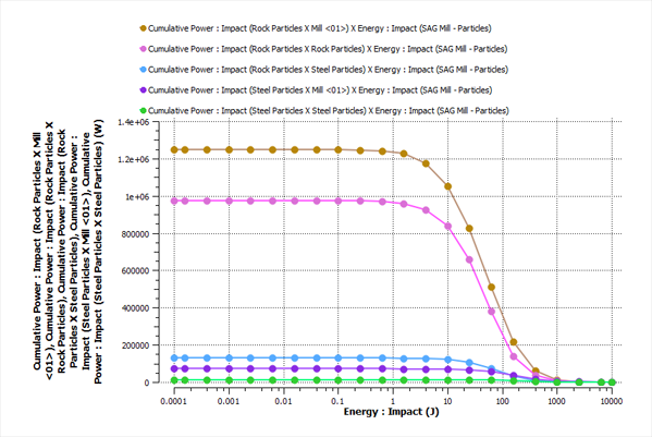
Contacts Energy Spectra curves can be displayed by Power, Cumulative Power (Figure 5), and Rate.
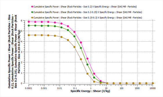
Figure 2.190: Examples of Contacts Impact Energy Spectra curves for various particle-to-particle and particle-to-geometry contact pairs
Tip: Refer to the DEM Technical Manual for implementation details. (From the Help menu, point to Manuals, and then click DEM Technical Manual.)
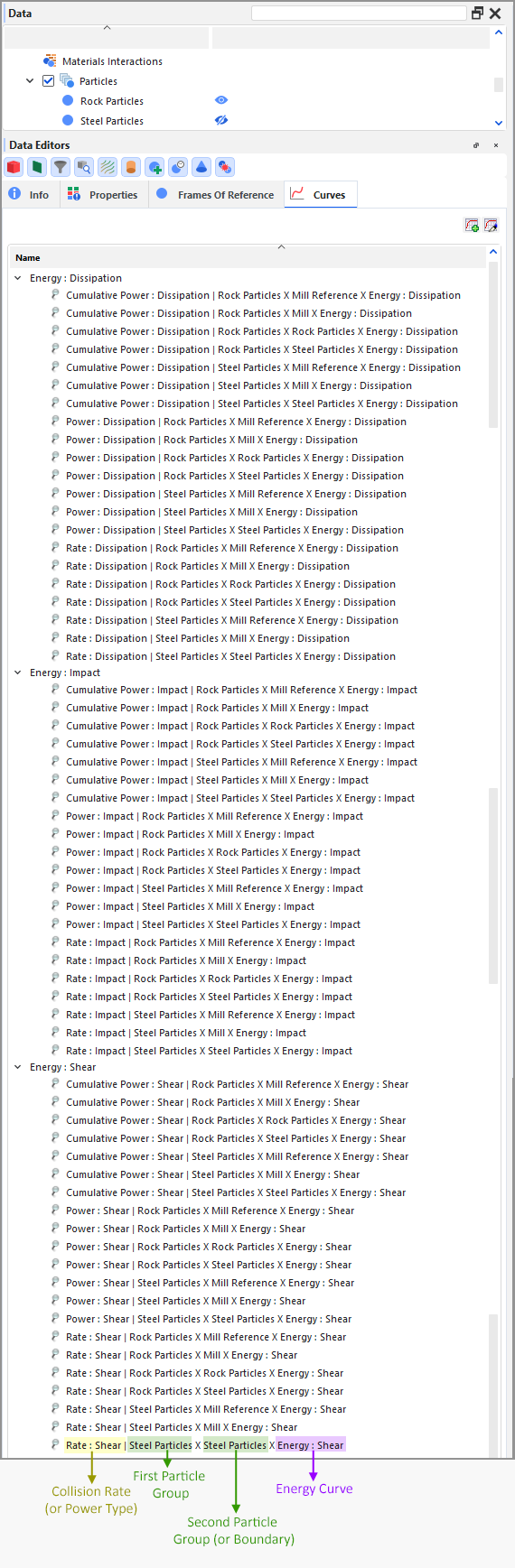
Viewing Contacts Energy Spectra
If prior to processing your simulation, you enabled Contacts Energy Spectra to be collected, then while the simulation is processing, Rocky calculates the selected energy curves (Dissipation, Impact, and/or Shear) for each pair of particle-to-particle or particle-to-geometry contact types, each generated by the power, cumulative power, and collisions rate (Figure 6).
You can then create a Cross plot of the Curves you are interested in analyzing (Figure 7).
Figure 2.192: Example cross plot of Contacts Energy Spectra showing both Cumulative Power and Power, for impact collisions between particles and geometries
About Opening Older Energy Spectra Projects
When opening projects that were created and processed in versions of Rocky prior to 2022 R1, Rocky will still read the energy spectra data in those projects and will display the energy spectra Curves as usual.
However, if you want to modify and then re-process an older energy spectra simulation in 2022 R1 or later versions, you will need to enable the energy spectra modules and define the type of collection parameters you want prior to processing the simulation.
The same is true for projects that you have created but not processed in older versions of Rocky; you must enable and define the energy spectra modules manually before processing your simulation.
Contacts Energy Spectra Collection Options
Use Figures 1-3 above and the tables below to understand how to collect contact-based energy statistics.
Table 1: Modules, Contacts Energy Spectra parameter definitions
|
Setting |
Description |
Range |
|---|---|---|
|
Dissipation Energy |
When enabled, collects contact-based statistics for dissipation energy, which is the fraction of the mechanical energy transformed irreversibly into other forms of energy during a collision. |
Turns on or off |
|
Impact Energy |
When enabled, collects contact-based statistics for impact energy, which is the maximum energy transferred during a collision. Tip: When Rocky simulates an actual breakage process (see also Enable and View Particle Breakage), this is usually the energy type considered to quantify the damage on the particles. |
Turns on or off |
|
Shear Energy |
When enabled, collects contact-based statistics for shear energy, which is the work done by the tangential contact forces during a collision. |
Turns on or off |
|
Number of Bins |
This defines how many sub-intervals the specified energy interval is evenly (using a logarithmic scale) subdivided. Determines the the resolution of the resulting Curves. The higher the value, the better the resolution. |
Positive values |
|
Maximum Energy |
This defines the right bound of the interval of energies that will be subdivided into bins for the construction of the energy spectra Curves. |
Positive values |
|
Minimum Energy |
This defines the left bound of the interval of energies that will be subdivided into bins for the construction of the energy spectra Curves. |
Positive values |
|
Start Time |
The amount of time you want to wait before starting to register energy spectra data. Tip: It is best practice to set your Start Time to begin after a steady state has been reached in your particle flow. |
Value must be positive but less than Simulation Duration, which is located on the Solver | Time sub-tab. (See also About Solver Parameters.) |
|
Time Delay after Release |
The amount of time you want to wait after a particle has been released before starting to register energy spectra data. |
Value must be positive but less than Simulation Duration, which is located on the Solver | Time sub-tab. (See also About Solver Parameters.) |
Table 2: Individual Geometry, Modules sub-tab parameter definitions
|
Setting |
Description |
Range |
|---|---|---|
|
Enable For This Geometry |
When enabled, the energy values involving this geometry will be recorded for energy spectra purposes. When cleared, the energy values involving this geometry will be ignored. |
Turns on or off |
Table 3: Individual Particle Group, Modules sub-tab parameter definitions
|
Setting |
Description |
Range |
|---|---|---|
|
Enable For This Particle Group |
When enabled, the energy values involving particles from this group will be recorded for energy spectra purposes. When cleared, the energy values involving particles from this group will be ignored. |
Turns on or off |
What would you like to do?
Learn more About Collecting Data
Learn more About Curves
See Also
ABOUT PARTICLES ENERGY SPECTRA
In Rocky, it is possible simulate the breakage behavior of particles. (See also Enable Particle Breakage Calculations.) However, simulations with breakage enabled can increase the computational cost, taking longer to process the simulation. With this in mind, Rocky has another feature you can use to analyze breakage: Particles Energy Spectra.
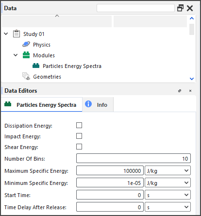
This useful tool collects different kinds of energy statistics per particle type and size category defined in its PSD, which can help predict breakage and attrition rates for continuous processes such as grinding mills. In this version of Rocky, these statistics are collected through the Particles Energy Spectra module (Figure 1).
This kind of energy spectra is often used in conjunction with Contacts Energy Spectra. (See also About Contacts Energy Spectra.)
See the sections below for more information about this type of energy statistic, and how it is collected, calculated, and viewed in Rocky.
About Collecting Particles-Based Energy Statistics
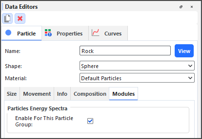
For particle-based analysis, relevant energy values associated to the collisions experienced by each individual particle collected during the simulation. In this version of Rocky, only particles belonging to particle groups that have been enabled for energy spectra collection will be recorded (Figure 2).
Figure 2.194: Additional module options for Particle groups when the Particles Energy Spectra module is enabled
Rocky then classifies and accumulates the associated specific energy values (energy per particle mass) according to a predefined set of energy levels, and represents the resulting cumulative values as curves.
For Particles Energy Spectra analysis, each particle group and particle size category will present a separate Energy Spectra curve. These curves are based upon three different types of collision energy, each of which can be useful for different types of analyses:
Dissipation Energy, which is the particle's mechanical energy transformed irreversibly into other forms of energy during a collision.
Impact Energy, which is the energy considered in breakage models for quantifying the damage on the particle's material that can lead to breakage. Tips: When Rocky simulates an actual breakage process (see also Enable and View Particle Breakage), this is usually the energy type considered to quantify the damage on the particles.
Shear Energy, which is the energy used to predict the abrasive wear of boundaries.
Because collecting statistics can take more processing time, memory, and disk storage due to increased file sizes, Rocky enables you to select which of these three particles energies you want to collect, and enables you to choose which particle groups will participate in energy spectra collection.
About Setting Time Delays
It is important to realize that data is only collected after both the Start Time and Time Delay After Release values are reached. Data begins being collected at the Start Time but only for the particles that were released before the Time Delay After Release value. This is to allow enough time for the particle flow within your simulation to reach a steady state before the energy spectra calculations begin.
For example, if the Start Time is 5s, and the Time Delay After Release is 3s, a particle entering the simulation at 4s will only be accounted for after 7s of simulation time.
Applications for Particles Energy Analysis
One common application of this type of analysis is for comminution devices like SAG mills (Figure 3), which use steel balls or other kinds of grinding media to help break rock or ore material into smaller fragments.
By looking at energy levels applied to particles, for instance, you can predict breakage rates.
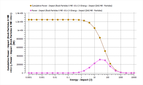
In the example shown in Figure 4 above, the Y-axis gives the Cumulative Specific Power : Impact values resulting from all collisions starting from the Start Time time you enter until the end of the simulated time (see also About Solver Parameters). The value of the Y-coordinate of a given point on the curve is obtained by dividing the cumulative specific energy by the time elapsed since the referred starting time. This value accounts for all collisions with a specific impact energy equal or higher than the specific energy given by its X-coordinate.
This kind of energy spectra curve is useful for the reason that all collisions with specific impact energy higher than a known threshold value may lead to particle breakage, while the remaining collisions will not, as shown in Figure 5 below. Therefore, the cumulative specific power available for breakage in that case will be given by the Y-coordinate in the curve, corresponding to the breakage threshold value.
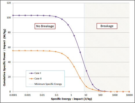
Important: This threshold value is the minimum value of impact energy that can break a particle, which is a known value derived from experiments. It will therefore change depending upon the material being simulated.
Tips:
Refer to the DEM Technical Manual for implementation details. (From the Help menu, point to Manuals, and then click DEM Technical Manual.)
To see a walk-through example of particles energy spectra being using to analyze breakage in a SAG mill, review Tutorial - SAG Mill in the Rocky Tutorial Guide.
Viewing Particles Energy Spectra
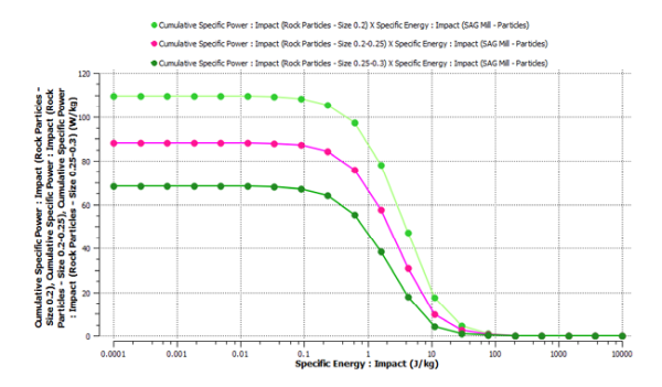
If prior to processing your simulation, you enabled Particles Energy Spectra to be collected, then while the simulation is processing, Rocky calculates the selected Cumulative Specific Power curves (Dissipation, Impact, and/or Shear) for each particle set, generated by each size of the particle size distribution, and separated by Specific Energy. These curves are grouped under Specific Energy on the Curves tab (Figure 6).

Using these curves, you can then create a Cross plot, similar to the example below (Figure 7).
About Opening Older Energy Spectra Projects
When opening projects that were created and processed in versions of Rocky prior to 2022 R2, Rocky will still read the energy spectra data in those projects and will display the energy spectra Curves as usual.
However, if you want to modify and then re-process an older energy spectra simulation in 2022 R2 or later versions, you will need to enable the energy spectra modules and define the type of collection parameters you want prior to processing the simulation.
The same is true for projects that you have created but not processed in older versions of Rocky; you must enable and define the energy spectra modules manually before processing your simulation.
Particles Energy Spectra Collection Options
Use Figures 1-2 above and the tables below to understand how to collect particle-based energy statistics.
Table 1: Modules, Particles Energy Spectra parameter definitions
|
Setting |
Description |
Range |
|---|---|---|
|
Dissipation Energy |
When enabled, collects particle-based statistics for dissipation energy, which is the fraction of the mechanical energy transformed irreversibly into other forms of energy during a collision. |
Turns on or off |
|
Impact Energy |
When enabled, collects particle-based statistics for impact energy, which is the maximum energy transferred during a collision. Tip: When Rocky simulates an actual breakage process (see also Enable and View Particle Breakage), this is usually the energy type considered to quantify the damage on the particles. |
Turns on or off |
|
Shear Energy |
When enabled, collects particle-based statistics for shear energy, which is the work done by the tangential contact forces during a collision. |
Turns on or off |
|
Number of Bins |
This defines how many sub-intervals the specified energy interval is evenly (using a logarithmic scale) subdivided. Determines the the resolution of the resulting Curves. The higher the value, the better the resolution. |
Positive values |
|
Maximum Specific Energy |
This defines the right bound of the interval of specific energies that will be subdivided into bins for the construction of the energy spectra Curves. |
Positive values |
|
Minimum Specific Energy |
This defines the left bound of the interval of specific energies that will be subdivided into bins for the construction of the energy spectra Curves. |
Positive values |
|
Start Time |
The amount of time you want to wait before starting to register energy spectra data. Tip: It is best practice to set your Start Time to begin after a steady state has been reached in your particle flow. |
Value must be positive but less than Simulation Duration, which is located on the Solver | Time sub-tab. (See also About Solver Parameters.) |
|
Time Delay after Release |
The amount of time you want to wait after a particle has been released before starting to register energy spectra data. |
Value must be positive but less than Simulation Duration, which is located on the Solver | Time sub-tab. (See also About Solver Parameters.) |
Table 2: Individual Particle Group, Modules sub-tab parameter definitions
|
Setting |
Description |
Range |
|---|---|---|
|
Enable For This Particle Group |
When enabled, the energy values involving particles from this group will be recorded for energy spectra purposes. When cleared, the energy values involving particles from this group will be ignored. |
Turns on or off |
What would you like to do?
Learn more About Collecting Data
Learn more About Curves
See Also
ENABLE AND VIEW DATA FOR CONTACTS ENERGY SPECTRA
Analyzing data for Contacts Energy Spectra involves first turning on the type of collection you want prior to processing the simulation (see also About Contacts Energy Spectra), and then determining which particle groups and geometries you want to involve in that collection. After processing your simulation you can then plot the resulting Curves (Figure 1).
It is important to realize that data is only collected after the Start Time value is reached.
For more details, tips, and limitations, see the About Contacts Energy Spectra topic.
To Enable and View Data for Contacts Energy Spectra:
Set up your simulation as you normally would (see also Set Simulation Parameters).
Before processing your simulation, do all of the following:
From the Data panel, select Modules, and then from the Data Editors panel, select Contacts Energy Spectra.
From the Data panel, under Modules, select the new Contacts Energy Spectra entry.
From the Data Editors panel, on the Contacts Energy Spectra tab, do all of the following:
Select one or more of the checkboxes for the type of energy statistics you want collected. (See also About Contacts Energy Spectra.) Important: You must select at least one checkbox in order for energy spectra to be collected.
In the Number of Bins box, enter the number of sub-intervals you want the energy interval to be evenly (using a logarithmic scale) subdivided.
In the Maximum Energy and Minimum Energy boxes, enter values for the right an left bounds of the interval of energies that will be subdivided into bins for the construction of the energy spectra Curves.
Set the values you want for both Start Time and Time Delay after Release. IMPORTANT: Because energy spectra is calculated as an average over time, it is important that you set this data to be collected after steady state has been reached.
For each geometry component that you do not want included in the collection of energy spectra, do the following:
From the Data panel, under Geometries select the geometry that you want to exclude from energy spectra collections.
From the Data Editors panel, select the Geometry | Modules tab and then under Contacts Energy Spectra clear the Enable For This Geometry checkbox.
For each particle group that you do not want included in the collection of energy spectra, do the following:
From the Data panel, under Particles select the particle group that you want to exclude from energy spectra collections.
From the Data Editors panel, select the Particle | Modules tab and then under Contacts Energy Spectra clear the Enable For This Particle Group checkbox.
Process your simulation as you normally would. (See also About Starting a Simulation.)
After your simulation reaches as least as far as the Start Time value, do the following:
From the Data panel, select Particles.
From the Data Editors panel, select the Curves tab.
Under the three Energy categories (Dissipation, Impact, and Shear), drag one or more of the Curves listed to the Workspace. (See also About Curves.) A new Cross Plot window is created showing the Curve(s) you selected.
From the Cross Plot window, do one or both of the following:
Modify the appearance of the Cross Plot. (See also About Changing the Appearance of a Graph (Plot or Histogram).) Tips: To show a Curve in a logarithmic format, right-click the desired axis and select Customize Axis. From the Axis tab, under Scale Options, enable the Logarithmic Scale checkbox.
Export the data to a CSV file. (See also Export Data into a CSV File.)
See Also:
ENABLE AND VIEW DATA FOR PARTICLES ENERGY SPECTRA
Analyzing data for Particles Energy Spectra involves first turning on the type of collection you want prior to processing (see also About Particles Energy Spectra), and then determining which particle groups you want to involve in that collection. After processing your simulation you can then plot the resulting Curves (Figure 1).
It is important to realize that data is only collected after the Start Time value is reached.
For more details, tips, and limitations, see the About Particles Energy Spectra topic.
To Enable and View Data for Particles Energy Spectra:
Set up your simulation as you normally would (see also Set Simulation Parameters).
Before processing your simulation, do all of the following:
From the Data panel, select Modules, and then from the Data Editors panel, select Particles Energy Spectra.
From the Data panel, under Modules, select the new Particles Energy Spectra entry.
From the Data Editors panel, on the Particles Energy Spectra tab, do all of the following:
Select one or more of the checkboxes for the type of energy statistics you want collected. (See also About Particles Energy Spectra.) Important: You must select at least one checkbox in order for energy spectra to be collected.
In the Number of Bins box, enter the number of sub-intervals you want the specific energy interval to be evenly (using a logarithmic scale) subdivided.
In the Maximum Energy and Minimum Energy boxes, enter values for the right an left bounds of the interval of specific energies that will be subdivided into bins for the construction of the energy spectra Curves.
Set the values you want for both Start Time and Time Delay after Release. IMPORTANT: Because energy spectra is calculated as an average over time, it is important that you set this data to be collected after steady state has been reached.
For each particle group that you do not want included in the collection of energy spectra, do the following:
From the Data panel, under Particles select the particle group that you want to exclude from energy spectra collections.
From the Data Editors panel, select the Particle | Modules tab and then under Particles Energy Spectra clear the Enable For This Particle Group checkbox.
Process your simulation as you normally would. (See also About Starting a Simulation.)
After your simulation reaches as least as far as the Start Time value, do the following:
From the Data panel, select Particles.
From the Data Editors panel, select the Curves tab.
Under the three Specific Energy categories (Dissipation, Impact, and Shear), drag one or more of the Curves listed to the Workspace. (See also About Curves.) A new Cross Plot window is created showing the Curve(s) you selected.
From the Cross Plot window, do one or both of the following:
Modify the appearance of the Cross Plot. (See also About Changing the Appearance of a Graph (Plot or Histogram).) Tip: To show a Curve in a logarithmic format, right-click the desired axis and select Customize Axis. From the Axis tab, under Scale Options, enable the Logarithmic Scale checkbox.
Export the data to a CSV file. (See also Export Data into a CSV File.)
See Also:
Use this section to quickly find and perform common tasks in Rocky.
What would you like to do?
Enter Input Variables or Mathematical Functions as Parameter Values
Change Set Up Parameters in a Partially Processed Simulation
Use the 1-Way Fluent Method to Process Fluent and Rocky Simulations
Use the 2-Way Fluent Method to Process Fluent and Rocky Simulations
Reuse 3D View Window, Workspace, and User Process Setups in Other Projects
See Also:
ENTER INPUT VARIABLES OR MATHEMATICAL FUNCTIONS AS PARAMETER VALUES
You can create Input variables in Rocky (see Defining Your Variables) and then use them in place of actual numerical values in situations where you want more flexibility. These variables can be used alone or within functions.
Tip: Rocky includes several visual feedback mechanisms, like text color, to help you ensure the variable names and mathematical functions you enter are correct. See Use Colored Text to Validate the Syntax of Your Entries for more information.
Important:Verify that your field units are set the way you want before using a variable-or function using a variable-within a field. Even though variables are always saved in the Variables list without units, as soon a variable-or function using a variable-is used within a parameter field, it takes on whatever units are currently set for that field and then those units are recorded for that specific usage in the Expressions list. Changing the units for the field after the variable or function have already been entered only converts the numerical display to reflect the new units; the original variable or function amount and units are still retained. However, you can change the units and value later by editing it in the Expressions list.
Most text fields in Rocky support entering variables or mathematical functions as parameter variables, including three-part text fields. There are a few exceptions to be aware of, however. (See also I cannot enter an input variable or mathematical function into a text field.)
Most of these parametric expressions will be retained while saving a copy of a project for restart purposes, but there are a few exceptions for some Start Time and Stop Time fields. (See also I get a "Links removed" message when I save my project for restart purposes.)
Most text fields will also support the entering of pre-defined mathematical functions (e.g., floor and pow) and constants (e.g., pi and e) that come standard with Python-based programs, including Rocky. And as such, these particular functions and constants cannot be used when defining Input variables.
What would you like to do?
See Also:
REPLACE A PARAMETER VALUE WITH A VARIABLE
Using the Data and Data Editors panels, locate and select the field for the parameter you want to replace, exactly enter the name of the variable you want to use, and then press Enter. The current value set for the variable in the Expressions/Variables panel is displayed in the field.
Tip: To see the units that are set for the variable you used, double click the value in the field. The units are displayed in brackets [ ] after the variable name.
Note: You cannot use pre-defined functions or constants to define your variable.
See Also:
REPLACE A PARAMETER VALUE WITH A FUNCTION USING A VARIABLE
Using the Data and Data Editors panels, locate and select the field for the parameter you want to replace, and then enter the function you want to use.
See Also:
REPLACE A PARAMETER VALUE WITH A PRE-DEFINED MATHEMATICAL CONSTANT
Using the Data and Data Editors panels, locate and select the field for the parameter you want to replace, and then enter the pre-defined mathematical function or constant you want to use.
See Also:
CHANGE THE SPEED OF A DEFAULT CONVEYOR
You can change the speed of a default receiving or feed conveyor at any point during the simulation. For example, you might want to measure reclaiming belt power by starting off a simulation with a feed conveyor stopped until a hopper is filled with particles, and then ending the simulation with the conveyor up to full speed.
TO CHANGE THE SPEED OF A DEFAULT CONVEYOR:
Ensure the default conveyor for which you want to change belt speed has already been added. (See also Add and Edit Geometry Components.)
From the Data panel, under Geometries, select the Receiving Conveyor or Feed Conveyor for which you want to change belt speed. The parameters for that geometry are displayed in the Data Editors panel.
From the Data Editors panel, on the Receiving Conveyor or Feed Conveyor tab, ensure the Belt Motion sub-tab is selected, and then do all of the following:
In the Belt Speed box, enter the full speed you want the belt to reach after acceleration is complete.
In the Beginning Start Time box, enter the amount of time that you want the simulation to run before the belt starts accelerating.
In the Acceleration Period box, enter the amount of time you want the belt to increase from full stop to full Belt Speed.
In the Beginning Stop Time box, enter the amount of time that you want the simulation to run before the belt starts decelerating.
In the Deceleration Period box, enter the amount of time that you want the belt to decrease from full Belt Speed to full stop.
See Also:
You change particle adhesion when you want a particle to act wetter or "stickier" than normal during a simulation. This might be useful in showing how ore flows through handling equipment during the wet season as compared to the dry, for example.
Tip: It is good practice to calibrate your particle settings to the real-world behavior of the material you are simulating before changing settings like adhesion. You may wish to use the Material Wizard and/or the Calibration Suite to help you with this task.
Set up the simulation as you normally would. (See also Setting Up a Simulation.)
During the Set Simulation-Wide Parameters step, ensure you select both the Rolling Resistance Model and the Adhesive Force you want from the Physics | Momentum tab. (See also About Physics Parameters.)
Adjust Materials Interactions values by doing all of following:
From the Data panel, select Materials Interactions.
From the Data Editors panel, choose the materials you want to modify from the Select Materials lists.
Adjust one or all of the settings provided including friction, adhesive distance, and force and/or stiffness fractions. (See also About Modifying Materials Interactions and Adhesion Values.)
Adjust Rolling Resistance values by doing all of the following:
From the Data panel, under Particles, select the rigid, convex Particle set for which you want to change adhesion.
From the Data Editors panel, select the Movement tab, and then adjust the Rolling Resistance value. Notes: - The Type C: Linear Spring Rolling Limit Rolling Resistance model is recommended for sticky particles. (See also About Physics Parameters.) - Rolling Resistance is not usually needed for shaped particles.
Process the simulation and then continue to adjust the Materials Interactions and Rolling Resistance values until you get the results you want.
See Also:
You set a particle size range-otherwise known as a Particle Size Distribution (PSD)-when you want particles of one shape but different sizes to be used in the simulation. If you set more than one size for a Particle set, Rocky uses a calculation to specify the distribution of sizes within any two dimensions you specify. This helps to more accurately reflect real matter.
When setting size ranges, the following three methods, or Size Types, can be used as a basis for defining your particle sizes (Figure 1):
Sieve Size (formerly "Sieve"), which for especially default Rocky shapes, bases particle size upon a virtual mesh hole just big enough for the particle to pass through. Note: Due to the way Sieve Size is calculated, it should be used only for even and balanced particle shapes (such as the default Solid particles included with Rocky) and not for fibers or shapes with high aspect ratios. (For more detail on how Sieve Size is calculated in Rocky, see the DEM Technical Manual. (From the Rocky Help menu, point to Manuals, and then click DEM Technical Manual.))
Equivalent Sphere Diameter (formerly "Equivalent Diameter"), which for especially irregular objects, bases particle size upon the diameter of a sphere with equivalent volume.
Tip: To see a walk-through example of setting and using Equivalent Sphere Diameter, refer to the following Tutorial: Tutorial - Windshifter in the Rocky Tutorial Guide. Original Size Scale, which for especially imported shapes, bases particle size upon the original size of the shape.
Tip: To see a walk-through example of setting and using Original Size Scale, refer to the following Tutorial: Tutorial - Tablet Coater in the Rocky Tutorial Guide.
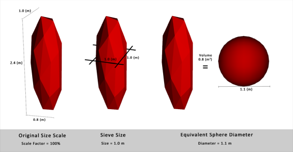
The PSD in Rocky is linear by Particle Mass or, on a semi-log scale, by Particle size and not by number. When you enter the percentage of cumulative mass and then either particle sieve Size, sphere Diameter, or original size Scale Factor (representing the three available Size Types, respectively), these represent points on a semi-log plot. Anything between two points follows the linear rule:

(See also About Adding and Editing Particle Sets.)
For example, if you specify 0.1 and 0.05 (m) particle sizes measured by sieve size, you will get a range of various particle sizes within those two dimensions.
Use the image and procedure below to set size ranges for your Particle sets.
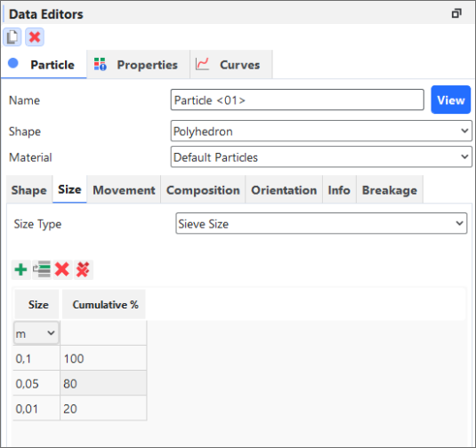
TO SET A PARTICLE SIZE RANGE OR PSD:
Ensure that the Particle set for which you want to specify size ranges has been added. (See also Add a New Particle Set.)
From the Data panel, select the Particle set you want (for example, Particle <01>) and then from the Data Editors panel, select the Size tab.
Set what you want for Size Type. (See also About Adding and Editing Particle Sets.)
Click the Add button once for each additional size range you require. Note: For rigid particles composed of Single Elements, there is no limit to the amount of rows you can add. For flexible or rigid particles composed of Multiple Elements (also known as *meshed* particles-see the Composition Tab section in the About Adding and Editing Particle Sets topic), only one row can be defined per Particle set.
Under Size, Diameter, or Scale Factor respectively, and starting with the first row, enter the maximum and minimum size values for each range in decreasing order. For example, to get a range of sieve sizes between 0.05-0.1 m and 0.01-0.05 m, enter 0.1, 0.05, and 0.01 in the first, second, and third rows respectively. (See Figure 2 above for example.) Note: The smallest value you enter (last row) will also be shown at that exact size (no range).
Under Cumulative %, starting with the second row, indicate what percentage of the total particle mass you want of that size value range by entering in decreasing order the previous row's percentage minus the percentage you want. For example, if you want 20% of the 0.05-0.1 m range, enter 80 (100-20); to get 60% of the 0.01-0.05 m range, enter 20 (80-20). (See Figure 2 above for example.)
Note: The percentage indicated in the final row also indicates what particle mass amount will be of that exact size (no range). For example, if the smallest size you enter is 0.01 m and you have entered 20 for Cumulative %, 20% of the particle mass will be exactly 0.01 m in size in addition to the ranges you have set.
See Also:
SEE SURFACE WEAR ON THE GEOMETRY ITSELF
There are two primary ways you can use Rocky to gain an understanding of how your geometries will wear over time. One way is by enabling surface wear modification, which changes the physical appearance of the geometry as the simulation progresses (Figure 1).
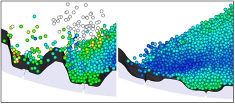
A second way is to turn on Boundary Collision Statistics (see also About Collision Statistics for Boundaries and then view a color map of the surface intensity (Figure 2), impact velocity, stresses, and more.
These features are independent of each other and are enabled from different areas of the Rocky UI. However, to view either type of wear data, you need to ensure that you have enabled enough geometry triangles prior to processing your simulation. Too few triangles will result in a jagged or blocky representation rather than a smooth one, but too many triangles can slow down your simulation.
Tip: To see a walk-through example of surface wear modification being using to analyze a SAG mill, review Tutorial - SAG Mill in the Rocky Tutorial Guide.
What would you like to do?
See Also:
ENABLE AND VIEW SURFACE WEAR MODIFICATION ON AN IMPORTED GEOMETRY
One way you can use Rocky to gain an understanding of how your geometries will wear over time is by enabling surface wear modification. Turning this feature on for an imported geometry prior to processing changes the physical appearance of the geometry as the simulation progresses (Figure 1).
To view this type of wear data, you must ensure that you have enabled enough geometry triangles prior to processing your simulation. Too few triangles will result in a jagged or blocky representation rather than a smooth one, but too many triangles can slow down your simulation.
It is important to realize that this data is only collected after the Wear Start value on the Solver | Time tab is reached. This is to allow enough time for the particle flow within your simulation to reach a steady state before surface wear modification calculations begin.
Tips: To see walk-through examples of surface wear modification, refer to the following Tutorials:
TO ENABLE AND VIEW SURFACE WEAR MODIFICATION:
Set up the simulation as you normally would. (See also Set Simulation Parameters). Tip: For easier comparison after the simulation is complete, consider including a copy of the imported geometry that will remain unworn. (See also Duplicate a Data Panel Item.)
Before processing the simulation, do all of the following:
From the Data panel, under Geometries, select the imported geometry for which you want to enable surface wear. The parameters for the geometry become active in the Data Editors panel.
From the Data Editors panel, on the Geometry tab, do all of the following:
From the Geometry sub-tab, ensure Triangle Size is small enough to enable the wear detail you want. (0.1 m is recommended for most chutes and mills).
From the Wear sub-tab, select the Wear Model you want to use, and then enter the Volume/Shear Work Ratio. Note: This is a calibration step that comes from real-world wear data you have collected on similar types of equipment.
From the Solver | Time tab, ensure that your Wear Start time is set to when you want wear data to be collected. (From the Data panel, select Solver and then from the Data Editors panel, locate this value on the Time sub-tab.) (See also About Solver Parameters.) Tip: It is best practice to set your Wear Start time to begin after a steady state has been reached for your particle flow.
Process the simulation as you normally would. (See also Processing a Simulation.)
From a 3D View window (see also About 3D View Windows), observe the changes to the surfaces of the geometry as the simulation progresses. Tip: If you included a copy of the original geometry in the simulation, you can use the unworn geometry as a comparison to one worn by surface wear modification.
Tips:
If you want to analyze the modified geometry outside of Rocky, you can choose to export it to an STL file. (See also Export a Geometry Component to an STL File.)
It is possible to save a copy of an in-process simulation with surface wear and have the wear calculations continue in the copy. (See also Save a Copy of a Partially Processed Simulation for Restart Purposes.) While you are unable to turn off wear calculations from the copy, if you no longer need wear, you can get around this by setting Volume/Shear Work Ratio to zero.
It is also possible to have wear calculations be made on replicated geometries.
See Also:
VIEW A COLOR MAP OF WEAR ON THE DEFAULT BELT OR IMPORTED GEOMETRY ITSELF
When you choose to turn on Boundary Collision Statistics (see also About Collision Statistics for Boundaries and enable wear-related categories such as Intensities, you are able to create and view a color map of the surface intensity (Figure 1), impact velocity, stresses, and more. These color maps can help you analyze the causes of excess wear on your conveyor belts or imported geometries.
TO VIEW A COLOR MAP OF WEAR ON THE DEFAULT BELT OR IMPORTED GEOMETRY ITSELF
Set up the simulation as you normally would. (See also Set Simulation Parameters.)
Before processing your simulation, ensure all of the following:
You have enabled the Boundary Collision Statistics that you want to be collected. (See also Enable and View Collision Statistics for Boundaries.)
You have verified that the default conveyor or imported geometry has its Triangle Size set small enough to enable the wear detail you want. (0.1 m is recommended for most chutes and mills). (From the Data panel under Geometry, select the component you want to verify. From the Data Editors panel, on the Geometry sub-tab, verify the Triangle Size value.)
Process the simulation as you normally would. (See also Processing a Simulation.)
Ensure you have a 3D View displayed in the Workspace. (See also Create and Modify a 3D View.)
When processing is complete enough to show the wear you want to visualize, from the first drop down list on the Coloring Settings toolbar, choose the data you want to display (e.g., Intensity.) The geometries in your simulation change color and a color legend is displayed in the 3D View.
Do any or all the following to adjust the view and color map details:
To better focus on the area you want to view, use the mouse to pan, rotate, and zoom. (See also About Using the Mouse and Keyboard to Change the View.)
To hide all items but the belt or geometry you want to focus on, use the eye icons to the left of the geometries and particles in the Data panel. (See also Show/Hide Components by Using Eye icons and Checkboxes.)
To modify the color bar, right-click the color legend and change the options listed. (See also About Color Scales.)
To focus on a different time period within the simulation, use the arrows or slider on the Time toolbar. (See also About the Time Toolbar.)
See Also:
USE THE 1-WAY FLUENT METHOD TO PROCESS FLUENT AND ROCKY SIMULATIONS
There are five main steps to using the 1-Way Fluent CFD Coupling method to process a 1-Way coupled Rocky and Ansys Fluent simulation, as described below.
Tips:
You may also complete this process from within Ansys Workbench. To accomplish this with transient Fluent data, however, there are separate steps you must follow. (See also Set Up and Run a 1-Way Fluent Transient Project within Ansys Workbench.)
You may also complete this process without using the Fluent UI. (See also Use a Journal to Run Fluent and Export Transient 1-Way Results.)
STEP I: VERIFY THAT ALL ROCKY-FLUENT PROGRAM REQUIREMENTS ARE MET
Before beginning Step II below, ensure all of the following program requirements have been met:
A Rocky-supported version of Ansys Fluent is installed upon a machine that also contains a Rocky program installation. (See also System Requirements.) Note: Rocky does not need Fluent to be installed on the same machine in order to run a 1-Way Fluent simulation. However, Fluent needs Rocky to be installed on the same machine in order for Rocky to enable the Rocky Export menu item in Fluent.
If you are not certain whether you have installed the Ansys Fluent Coupling Support component during Rocky installation, first follow the Install Ansys Coupling Components procedure before beginning Step II.
STEP II: SET UP, PROCESS, AND THEN EXPORT THE CFD SIMULATION
In Ansys Fluent, set up the CFD simulation that you want to couple with Rocky. Important: Ensure that you complete all of the following; these exact settings are required for 1-Way Fluent coupled simulations:
From the Fluent Launcher dialog, do the following:
Under Dimension ensure 3D is selected.
Under Options select Double Precision.
From the Solution Methods tab, under Pressure-Velocity Coupling Scheme, ensure SIMPLE is selected.
Optional Steps:
If you want to use any standard Fluent post processing options, set them up now before processing the simulation.
If you want both sides of your coupled simulation to share identical geometries, set up those geometries now in Fluent, but be sure you save your Fluent Case File. Later in Rocky, you can choose to import those geometries directly from the CAS, CAS.H5, or CAS.GZ file that you will save from Fluent in the next step.
If you want both sides of your coupled simulation to share the same geometry movements, set up the translation or rotation movements now using Fluent Moving Meshes. These movements will later be imported (with the F2R file) into Rocky (Step IV.2 below), which will automatically convert them into Rocky Motion Frames. Note: If you chose to define your moving meshes in Fluent using expressions, you will need to set up your Motion Frames in Rocky manually. (See also Step IV.2 below and About Creating and Applying Motion Frames to Imported Geometries.)
From the File menu, Write the case to a location of your choosing. Tip: Remember the location of this directory as you will need to access files saved to it in later steps.
(Optional) Configure the options for Rocky Export by doing any or all of the following:
Define the directory you want to export by doing the following:
From the Fluent Rocky Export menu, point to Configure one-way export and then click Select Directory to Export.
From the Select folder to write fluent to rocky files, select the folder to where you want your fluid data saved, and then click Select Folder. Note: If you do not define this, Fluent will automatically use the same folder as your case file.
Define the additional variables you want to export by doing the following: Note: These additional variables can include static pressure, species variables such as mole fraction, diffusivity, and user defined memories. Other variables such as Velocity, Pressure Gradient, Temperature, and Fluid properties are always exported no matter what you select here.
From the Fluent Rocky Export menu, point to Configure one-way export and then click Select Variables to Export. Note: To do this task, you must first have variables defined within Fluent.
From the Additional Variables Selector dialog that appears, select the variables that you want included in the exported files, and then click OK.
Define how frequently you want files to be saved during the export by doing the following:
From the Fluent Rocky Export menu, point to Configure one-way export and then click Set Output Frequency.
b. From the Fluent to Rocky (F2R) time-step multiplier dialog define what you want for the F2R Time Step Multiplier value, and then click OK. Note: Only whole numbers are valid multipliers.
Export the data you want by doing one of the following:
To export steady-state data, do the following:
Process the CFD simulation until the fluid flow reaches a steady state.
From the Fluent Rocky Export menu, point to Export one-way data and then click Export current data to Rocky. Tips:
If you do not see this menu in Fluent, then first follow the Install Ansys Coupling Components procedure before continuing.
To perform this step before the Fluent case is done processing, stop Fluent from processing the case further before using Rocky Export menu.
An F2R and other files needed for coupling is saved to the same folder as your Fluent case file (or the alternate folder you defined in step 3).
To export transient data, do the following:
Begin the export process by doing one of the following:
To start recording from the initial conditions (without any prior Fluent results), initialize the Fluent case.
To start recording some time after Fluent results have been collected, process the CFD simulation until the fluid flow reaches the point that you want to start recording data, and then stop Fluent from processing the case further.
From the Fluent Rocky Export menu, point to Record one-way transient data, and then click Start one-way transient export. Tip: If you do not see this menu in Fluent, then first follow the Install Ansys Coupling Components procedure before continuing.
Begin (or resume) processing in Fluent until the point you want to stop recording data. Stop Fluent from processing the case.
From the Fluent Rocky Export menu, point to Record one-way transient data, and then click Stop one-way transient export. An F2R and other files needed for coupling is saved to the same folder as your Fluent case file (or the alternate folder you defined in step 3).
Click OK to close the confirmation message dialog.
Save the Fluent case again.
STEP III: SET UP THE DEM SIMULATION IN ROCKY
In Rocky, set up your simulation project as you normally would. (See also Set Simulation Parameters.) Tips:
If you want to use the exact same geometries as in the Fluent simulation, you may choose to import the CAS, CAS.H5, or CAS.GZ file you generated in Step II, which will include all available geometries as separate components.
If you enabled Energy Equations in the Fluent case, then ensure you also enable Thermal Modeling settings in Rocky. (See also Enable Thermal Modeling Calculations.)
STEP IV: APPLY 1-WAY FLUENT COUPLING
From the Data panel, click CFD Coupling and then from the Data Editors panel, choose Fluent (Fluid → Particle) from the Coupling Mode list.
From the Select Fluent 2 Rocky export file dialog, locate and select the F2R file you exported in Step II, and then click Open. A new 1-Way Fluent item appears beneath CFD Coupling in the Data panel. Important:For F2R files that include transient data, this step could take several minutes to complete. In addition, if you chose to set up Moving Meshes in Fluent, one new Frame will appear under Motion Frames in the Data panel for each Cell Zone with motions you have defined. Important:If you have defined your Moving Meshes in Fluent using expressions, Rocky will not be able to create the associated Motion Frames for you automatically. Rather, you must manually create your own Motion Frames in Rocky to match the Fluent motions as closely as possible. Tip: To save loading time, the Nodes for the imported fluid are turned off by default in the 3D View. To see them, from the Coloring tab, enable the Nodes checkbox. (See also About Using the Coloring Tab to Change a 3D View.)
Under CFD Coupling, select the new item and then from the Data Editors panel, on the 1-Way Fluent tab, do the following:
Set the Start Time you want.
From the Interactions tab, do the following:
From the Particle list, select (or multi-select) the Particle set name(s) for which you want to define interactions, and then select the various CFD laws you want for the selected set(s).
Select what you want for Turbulent Dispersion.
(See also About Using the 1-Way Fluent Method.)
STEP IV: PROCESS THE COUPLED SIMULATION
In Rocky, process the simulation as you normally would. (See also Start Processing a Simulation from the Beginning.)
See Also:
USE THE 2-WAY FLUENT METHOD TO PROCESS A FLUENT AND ROCKY SIMULATION
There are five main steps to using the 2-Way Fluent method to process a coupled Rocky and Ansys Fluent simulation, as described below.
Note: Both Single phase and Multiphase approaches are covered in this procedure.
Step I: Verify that All Rocky-Fluent Program Requirements are Met
Before beginning Step II below, ensure all of the following program requirements have been met:
A Rocky-supported version of Ansys Fluent is installed upon the same machine that contains your Rocky program installation. (See also System Requirements.)
If you desire to run Fluent as a parallel process (rather than a serial one), then the machine upon which you intend to run the Rocky portion of your coupled simulation must also run at least the host part of the Fluent process. (For more information about how the processing architecture works in Fluent, refer to your Ansys Fluent documentation.)
If you are not certain whether you have installed the Ansys Fluent Coupling Support component during Rocky installation, first follow the Install Ansys Coupling Components procedure before beginning Step II.
Step II: Set Up the Initial CFD Simulation
In Ansys Fluent, set up the CFD simulation that you want to couple with Rocky. Important:Ensure that you complete all of the following; these exact settings are required for 2-Way Fluent coupled simulations:
From the Fluent Launcher dialog, do the following:
Under Dimension ensure 3D is selected.
Under Options select Double Precision.
From the General tab, under Time select Transient.
From the Tree panel, expand Models, and then do one of the following:
To set up a CFD project with a single fluid phase, ensure that Multiphase model is set to Off.
Otherwise, to set up a CFD project with two or more fluid phases, do all of the following:
Under Models, select Eulerian. Note: The Volume of Fluid model is not supported by Rocky in this version.
Under Eulerian Parameters, keep all options cleared. (All are unsupported with coupling, including the Multi-Fluid VOF Model.)
Under Volume Fraction Parameters, select Implicit for Formulation.
Under Number of Eulerian Phases, select the number of phases that includes an additional one for particles. (The number of Eulerian phases should be set to number of fluid phases + 1.).
Click OK.
Only for projects where the Multiphase model has been set to Eulerian (i.e., multiphase simulations), ensure that you set the additional particle phase to have a different material from the primary phase.
Only for projects involving multiple fluid species, for the mixture-template for your Material Mixture, ensure that you have enabled Species Transport. Important:The species you list last in the Selected Species list is very important as Fluent considers it to be the bulk species; this last species, therefore, will not result in a mass source term from Rocky.
From the Solution Methods tab, under Pressure-Velocity Coupling Scheme, do one of the following:
For projects where the Multiphase model has been set to Eulerian (i.e., multiphase simulations), you must ensure that the Phase Coupled SIMPLE method is selected.
For projects where the Multiphase model has been set to Off (i.e., single phase simulations), you may choose any pressure-velocity coupling scheme that works for your particular application.
From the Solution Methods tab, under Transient Formulation, ensure that First Order Implicit is selected.
From the Run Calculation tab, under Time Advancement, do the following:
Set Type to Fixed.
Ensure the Time Step Size value you set matches the minimum initial Output Frequency you want for your Rocky and Fluent files. Tip: You can change the outputs to be less frequent than this minimum in your Rocky setup later.
Tip: To help ensure that you perform these setup steps correctly, please refer to the CFD Coupling Technical Manual document (from the Help menu, point to Manuals, and then click CFD Coupling Technical Manual). For single-phase approaches, you may also follow the self-guided:
Tutorial 14 - DEM-CFD Two-Way Coupling with Ansys Fluent.
Optional Steps:
If you want to start your Rocky simulation with a given initial fluid flow, save the solution in Fluent as a standard DAT (DAT.H5 or DAT.GZ) file to be used by Rocky later (see Step IV below). Note: If your simulation is multiphase, ensure that the secondary phase (particulate phase) has a volume fraction of zero set before saving your DAT (DAT.H5 or DAT.GZ) file. Later, after the simulation is initialized, the initial particulate volume fraction will be calculated in Rocky according to the particles enabled at the beginning of the simulation.
If you want to use any standard Fluent post processing options, set them up now before processing the simulation.
If you want both sides of your coupled simulation to share identical geometries, set up those geometries now in Fluent, but be sure you save your Fluent Case File. Later in Rocky, you can choose to import those geometries directly from the CAS, CAS.H5, or CAS.GZ file that you will save from Fluent in the next step.
If you want both sides of your coupled simulation to share the same geometry movements, set up the translation or rotation movements now using Fluent Moving Meshes. These movements will later be imported (with the CAS, CAS.H5, or CAS.GZ file) into Rocky (Step IV.2 below), which will automatically convert them into Rocky Motion Frames. Note: If you chose to define your moving meshes in Fluent using expressions, you will need to set up your Motion Frames in Rocky manually. (See also Step IV.2 below and About Creating and Applying Motion Frames to Imported Geometries.)
Write the completed CFD setup to a CAS (CAS.H5 or CAS.GZ) file.
Step III: Set up the Initial Rocky Simulation
In Rocky, set up your simulation project as you normally would. (See also Set Simulation Parameters.) Tip: If you want to use the exact same geometries as in the Fluent simulation, you may choose to import the CAS, CAS.H5, or CAS.GZ file you generated in Step II, which will include all available geometries as separate components.
Recommended: Save your Rocky project to the same folder in which you saved the CAS (CAS.H5 or CAS.GZ) file in Step II. (See also Save a New Simulation Project.)
Whether or not you choose to take this step, Rocky will create its own copy of the CAS (CAS.H5 or CAS.GZ).
Optional: If you want to start your coupled simulation with particle data already in the system, do all of the following:
Process the simulation as you normally would, without CFD coupling. (See also Start Processing a Simulation from the Beginning.)
After processing is complete, from the File menu, click Save project as….
From the Save As dialog, choose the third option, "Save as a New Project for Restart", and then click OK.
In the Save in list, choose the same location in which you saved the CAS (CAS.H5 or CAS.GZ) file in Step II, verify the File Name, and then click Save.
From the Data panel, click CFD Coupling and then from the Data Editors panel, choose 2-Way Fluent from the Coupling Mode list.
From the Select Fluent CAS file dialog, locate and select the CAS (CAS.H5 or CAS.GZ) file you generated in Step II, and then click Open. Important:A mesh validation step will occur immediately after the CAS file import. This requires a valid Fluent license on the same machine upon which you are running the Rocky simulation. After successful import, a new 2-Way Fluent item appears beneath CFD Coupling in the Data panel. In addition, if you chose to set up Moving Meshes in Fluent, one new Frame will appear under Motion Frames in the Data panel for each Cell Zone with motions you have defined. Important:If you have defined your Moving Meshes in Fluent using expressions, Rocky will not be able to create the associated Motion Frames for you automatically. Rather, you must manually create your own Motion Frames in Rocky to match the Fluent motions as closely as possible.
If the CAS (CAS.H5 or CAS.GZ) file imported new Motion Frames, assign each newly imported Frame to the geometry component you want to share corresponding movements with Fluent. (See also Apply a Motion Frame to an Imported Geometry.)
From the Data panel under CFD Coupling, select the new 2-Way Fluent item and then from the Data Editors panel, do all of the following:
From the Interactions tab, define the CFD laws you want per *Particle set* by selecting (or multi-selecting) the set name(s) from the Particle list, and then defining the laws you want for the selected set(s). From this tab, you can also set the Turbulent Dispersion options for the entire coupled simulation. (See also About Using the 2-Way Fluent Method.)
From the Coupling tab, define the Mapping Method and Sub-Stepping options you want.
From the Zones and Interfaces tab, do the following:
Select one or more options from the Coupling Fluid Cell Zone list.
(Optional) If provided, select the options you want from the Mapping Cell Zone Interfaces list.
From the Fluent tab, do all of the following:
Important: If your Fluent case is multiphase, from the Rocky Phase list, ensure that the phase representing particle flow is chosen.
Choose what fluid flow data Rocky starts with by doing one of the following:
To start your Rocky simulation without providing initial fluid flow data, ensure the Use Data Initialization checkbox remains cleared. Doing so ensures that the initialization settings prescribed in Fluent will be used to generate the initial fluid flow.
To start your Rocky simulation with initial fluid flow data, select Use Data Initialization, click the Import File button, and then select and open the DAT (DAT.H5 or DAT.GZ) file you saved in Step II. Important:If you chose to use initial fluid flow data in your simulation and your simulation is multiphase, you must have ensured that the secondary phase (particulate phase) had a volume fraction of zero set before you saved your DAT (DAT.H5 or DAT.GZ) file. This is important because later, after the simulation is initialized, the initial particulate volume fraction will be calculated in Rocky according to the particles enabled at the beginning of the simulation.
From the Version list, select what Ansys version you want to use for fluid coupling. Tip: If you do not see the Ansys version you expected, see also Rocky does not list my Ansys version when I try to set up 2-Way Fluent Coupling.
Choose how the fluid portion of the simulation is processed by doing one of the following:
To have it processed on only one processor on your local machine, from the Execution mode list, select Serial.
To have it processed on multiple processors on your local machine, from the Execution mode list, select Local Parallel and then from the Solver Processes field, enter the number of processors you want to dedicate to the CFD solver.
To have it processed across several machines on your network, from the Execution mode list, select Distributed Parallel and then do one of the following:
Under Hosts, click the Add button for each server you want to add and then for each row, define the Host name and Amount information.
To import an external list of hosts and amounts that you created outside of Rocky, click the Import File button, and then from the Import dialog, locate and select the TXT file containing the information, and then click Open. The Host section is populated with the information from the TXT file. Tip: The format for the TXT file needs to include the Host name repeated on separate lines for each Amount you want devoted. To see an example, create a few sample rows as specified directly above, click Export File and then save and view the results as a TXT file.
Choose how many Fluent files to keep by doing one of the following:
To keep each Fluent DAT (DAT.H5 or DAT.GZ) file (and in some cases, as with moving meshes, CAS files as well) for every Rocky output file that is saved, enable the Keep all files checkbox. Important:Unless you require all files for post-processing in Fluent, keeping all files is not recommended for the 2-Way Fluent method. (See also About Using the 2-Way Fluent Method.)
To keep only the last (or last several) Fluent DAT (DAT.H5 or DAT.GZ) files (and in some cases, CAS files) saved, ensure the Keep all files checkbox is cleared, and then enter the number of last-saved files you want to keep in the Files to keep box. Tip: Keeping the last 2 (or more) files is recommended. Important:If you decide to save fewer than all of the files, be aware that you will not be able to post-process the unsaved files in Fluent. Also, be aware that the number DAT (and in some cases, CAS) files you save will be as far back in time as you can restart your simulation since fluid data will not be available for prior times. Tip: You can also choose which quantities and frequency you want to write to disk using Fluent's Autosave functionality.
From the Variables tab, review the Additional Inputs and Additional Outputs (if applicable) that Rocky and Fluent will exchange during the coupled simulation. Tip: If you have enabled species transport, this is where the per-species variables Fluent provides Rocky, and the mass source terms Rocky provides Fluent will be listed.
Tips:
To verify or change the CAS (CAS.H5 or CAS.GZ) file selected, click Open (at the bottom of the 2-Way Fluent | Fluent tab) and Rocky will open its own copy of the CAS (CAS.H5 or CAS.GZ) file in Fluent. From here, you can view or make changes to the Rocky copy of the file. Important:Because Rocky uses only its own copy of the imported CAS (CAS.H5 or CAS.GZ) file, it is critical that you only open the imported CAS (CAS.H5 or CAS.GZ) from Rocky's Open button, and that you save any changes to the default location Rocky indicates.
If you make changes to the Rocky copy of the CAS (CAS.H5 or CAS.GZ) file in Fluent, click Refresh to have Rocky include the updates. Important:The Refresh button works only if you first opened the CAS (CAS.H5 or CAS.GZ) file from the Rocky Open button located at the bottom of the 2-Way Fluent | Fluent tab.
If you made changes to your original Fluent version of the CAS (CAS.H5 or CAS.GZ) file and did not use the Rocky Open button as specified above, you must set the CFD Coupling option to No Coupling to clear the values, and then restart "Step IV: Apply 2-Way Coupling" again from the beginning, selecting the updated CAS (CAS.H5 or CAS.GZ) file in step 2.
Step V: Process the Coupled Simulation
In Rocky, process the simulation as you normally would (see also Start Processing a Simulation from the Beginning) with the following exception:
Keeping in mind the Time Step Size value you set in Fluent, from the Solver | Time tab, set what you want for Fluent Outputs Multiplier. Tip: You can see how this change affects Rocky's Output Frequency in the disabled Simulation field.
Rocky automatically opens Ansys Fluent and the Fluent simulation is processed at the same time as the Rocky simulation, depending upon the limitations of your Ansys license. If any incompatibility is found between the Fluent setup and Rocky, an error will be shown in Rocky with additional information. Once the simulations are complete, the data from both are available to see and analyze however you choose. (See also Analyzing a Simulation.)
See Also:
USE THE 2-WAY FLUENT SEMI-RESOLVED METHOD TO PROCESS A FLUENT AND ROCKY SIMULATION
There are five main steps to using the 2-Way Fluent Semi-Resolved method to process a coupled Rocky and Ansys Fluent simulation, as described below.
Note: Both Single phase and Multiphase approaches are covered in this procedure.
Step I: Verify that All Rocky-Fluent Program Requirements are Met
Before beginning Step II below, ensure all of the following program requirements have been met:
A Rocky-supported version of Ansys Fluent is installed upon the same machine that contains your Rocky program installation. (See also System Requirements.)
If you are not certain whether you have installed the Ansys Fluent Coupling Support component during Rocky installation, first follow the Install Ansys Coupling Components procedure before beginning Step II.
Step II: Set Up the Initial CFD Simulation
Important: When setting up your 3D mesh, ensure that only tetrahedron, prism, pyramid, or hexahedron cell types are used. Note: Polyhedral mesh cells, including the CutCell type, are not supported in this version.
In Ansys Fluent, set up the CFD simulation that you want to couple with Rocky. Important: Ensure that you complete all of the following; these exact settings are required for 2-Way Fluent Semi-Resolved
coupled simulations:
From the Fluent Launcher dialog, do the following:
Under Dimension ensure 3D is selected.
Under Options select Double Precision.
From the General tab, under Time select Transient.
From the Tree panel, expand Models, and then do one of the following:
To set up a CFD project with a single fluid phase, ensure that Multiphase model is set to Off.
Otherwise, to set up a CFD project with two or more fluidphases, do all of the following:
Under Models, select Eulerian.
Under Number of Eulerian Phases, select the number of phases you need. Note: Unlike with the standard 2-Way Fluent method, you do not need an additional phase for particles with this method.
Click OK.
From the Solution Methods tab, under Pressure-Velocity Coupling Scheme, you may choose any pressure-velocity coupling scheme that works for your particular application.
From the Solution Methods tab, under Transient Formulation, ensure that First Order Implicit is selected.
From the Run Calculation tab, under Time Advancement, do the following:
Set Type to Fixed.
Ensure the Time Step Size value you set is aligned with the Output Settings | Time Interval value you want to set later in Rocky. Tip: To ensure that your post-processing is better aligned between the two products, it is recommended that the Time Step Size in Fluent and the Output Settings | Time Interval value in Rocky are multiples.
Optional Steps:
If you want to start your Rocky simulation with a given initial fluid flow, save the solution in Fluent as a standard DAT (DAT.H5 or DAT.GZ) file to be used by Rocky later (see Step IV below).
If you want to use any standard Fluent post processing options, set them up now before processing the simulation.
If you want both sides of your coupled simulation to share identical geometries, set up those geometries now in Fluent, but be sure you save your Fluent Case File. Later in Rocky, you can choose to import those geometries directly from the CAS, CAS.H5, or CAS.GZ file that you will save from Fluent in the next step.
If you want both sides of your coupled simulation to share the same geometry movements, set up the translation or rotation movements now using Fluent Moving Meshes. These movements will later be imported (with the CAS, CAS.H5, or CAS.GZ file) into Rocky (Step IV.2 below), which will automatically convert them into Rocky Motion Frames. Note: If you chose to define your moving meshes in Fluent using expressions, you will need to set up your Motion Frames in Rocky manually. (See also Step IV.2 below and About Creating and Applying Motion Frames to Imported Geometries.)
Write the completed CFD setup to a CAS (CAS.H5 or CAS.GZ) file.
Step III: Set up the Initial Rocky Simulation
In Rocky, set up your simulation project as you normally would. (See also Set Simulation Parameters.)
Tip: If you want to use the exact same geometries as in the Fluent simulation, you may choose to import the CAS, CAS.H5, or CAS.GZ file you generated in Step II, which will include all available geometries as separate components.
Note: 2-Way Fluent Semi-Resolved currently supports only the following particle shapes: Spheres, Shells (either rigid or flexible), or Custom Imported Polyhedrons (rigid only).
Recommended: Save your Rocky project to the same folder in which you saved the CAS (CAS.H5 or CAS.GZ) file in Step II. (See also Save a New Simulation Project.) Whether or not you choose to take this step, Rocky will create its own copy of the CAS (CAS.H5 or CAS.GZ).
Optional: If you want to start your coupled simulation with particle data already in the system, do all of the following:
Process the simulation as you normally would, without CFD coupling. (See also Start Processing a Simulation from the Beginning.)
After processing is complete, from the File menu, click Save project as….
From the Save As dialog, choose the third option, "Save as a New Project for Restart", and then click OK.
In the Save in list, choose the same location in which you saved the CAS (CAS.H5 or CAS.GZ) file in Step II, verify the File Name, and then click Save.
Step IV: Apply 2-Way Fluent Semi-Resolved Coupling
From the Data panel, click CFD Coupling and then from the Data Editors panel, choose Fluent Semi-Resolved from the Coupling Mode list.
From the Select Fluent CAS file dialog, locate and select the CAS (CAS.H5 or CAS.GZ) file you generated in Step II, and then click Open. Important:A mesh validation step will occur immediately after the CAS file import. This requires a valid Fluent license on the same machine upon which you are running the Rocky simulation. After successful import, a new 2-Way Fluent Semi-Resolved item appears beneath CFD Coupling in the Data panel. In addition, if you chose to set up Moving Meshes in Fluent, one new Frame will appear under Motion Frames in the Data panel for each Cell Zone with motions you have defined. Important:If you have defined your Moving Meshes in Fluent using expressions, Rocky will not be able to create the associated Motion Frames for you automatically. Rather, you must manually create your own Motion Frames in Rocky to match the Fluent motions as closely as possible.
If the CAS (CAS.H5 or CAS.GZ) file imported new Motion Frames, assign each newly imported Frame to the geometry component you want to share corresponding movements with Fluent. (See also Apply a Motion Frame to an Imported Geometry.)
From the Data panel under CFD Coupling, select the new 2-Way Fluent Semi-Resolved item and then from the Data Editors panel, do all of the following:
Choose what fluid flow data Rocky starts with by doing one of the following:
To start your Rocky simulation without providing initial fluid flow data, ensure the Use Data Initialization checkbox remains cleared. Doing so ensures that the initialization settings prescribed in Fluent will be used to generate the initial fluid flow.
To start your Rocky simulation with initial fluid flow data, select Use Data Initialization, click the Import File button, and then select and open the DAT (DAT.H5 or DAT.GZ) file you saved in Step II.
From the Version list, select what Ansys version you want to use for fluid coupling. Tip: If you do not see the Ansys version you expected, see also Rocky does not list my Ansys version when I try to set up 2-Way Fluent Coupling.
Choose how the fluid portion of the simulation is processed by doing one of the following:
To have it processed on only one processor on your local machine, from the Execution mode list, select Serial.
To have it processed on multiple processors on your local machine, from the Execution mode list, select Local Parallel and then from the Solver Processes field, enter the number of processors you want to dedicate to the CFD solver.
To have it processed across several machines on your network, from the Execution mode list, select Distributed Parallel and then do one of the following:
Under Hosts, click the Add button for each server you want to add and then for each row, define the Host name and Amount information.
To import an external list of hosts and amounts that you created outside of Rocky, click the Import File button, and then from the Import dialog, locate and select the TXT file containing the information, and then click Open. The Host section is populated with the information from the TXT file. Tip: The format for the TXT file needs to include the Host name repeated on separate lines for each Amount you want devoted. To see an example, create a few sample rows as specified directly above, click Export File and then save and view the results as a TXT file.
Choose how many Fluent files to keep by doing one of the following:
To keep each Fluent DAT (DAT.H5 or DAT.GZ) file (and in some cases, as with moving meshes, CAS files as well) saved, enable the Keep all files checkbox. Important:Unless you require all files for post-processing in Fluent, keeping all files is not recommended for the 2-Way Fluent Semi-Resolved method. (See also About Using the 2-Way Fluent Semi-Resolved Method.)
To keep only the last (or last several) Fluent DAT (DAT.H5 or DAT.GZ) files (and in some cases, CAS files) saved, ensure the Keep all files checkbox is cleared, and then enter the number of last-saved files you want to keep in the Files to keep box. Tip: Keeping the last 2 (or more) files is recommended. Important:If you decide to save fewer than all of the files, be aware that you will not be able to post-process the unsaved files in Fluent. Also, be aware that the number of DAT (and in some cases, CAS) files you save will be as far back in time as you can restart your simulation since fluid data will not be available for prior times. Tip: You can also choose which quantities and frequency you want to write to disk using Fluent's Autosave functionality.
Tips:
To verify or change the CAS (CAS.H5 or CAS.GZ) file selected, click Open and Rocky will open its own copy of the CAS (CAS.H5 or CAS.GZ) file in Fluent. From here, you can view or make changes to the Rocky copy of the file. Important:Because Rocky uses only its own copy of the imported CAS (CAS.H5 or CAS.GZ) file, it is critical that you only open the imported CAS (CAS.H5 or CAS.GZ) from Rocky's Open button, and that you save any changes to the default location Rocky indicates.
If you make changes to the Rocky copy of the CAS (CAS.H5 or CAS.GZ) file in Fluent, click Refresh to have Rocky include the updates. Important:The Refresh button works only if you first opened the CAS (CAS.H5 or CAS.GZ) file from the Rocky Open button.
If you made changes to your original Fluent version of the CAS (CAS.H5 or CAS.GZ) file and did not use the Rocky Open button as specified above, you must set the CFD Coupling option to No Coupling to clear the values, and then restart "Step IV: Apply 2-Way Fluent Semi-Resolved Coupling" again from the beginning, selecting the updated CAS (CAS.H5 or CAS.GZ) file in step 2.
Step V: Process the Coupled Simulation
In Rocky, process the simulation as you normally would (see also Start Processing a Simulation from the Beginning) with the following exception:
Keeping in mind the Time Step Size value you set in Fluent, from the Solver | Time tab, set what you want for Output Settings | Time Interval. Tip: To ensure that your post-processing is better aligned between the two products, it is recommended that the Time Step Size in Fluent and the Output Settings | Time Interval value in Rocky are multiples.
Rocky automatically opens Ansys Fluent and the Fluent simulation is processed at the same time as the Rocky simulation, depending upon the limitations of your Ansys license. If any incompatibility is found between the Fluent setup and Rocky, an error will be shown in Rocky with additional information. Once the simulations are complete, the data from both are available to see and analyze however you choose. (See also Analyzing a Simulation.)
See Also:
ENABLE AND VIEW PARTICLE BREAKAGE
Analyzing either Instantaneous or Discrete particle breakage in Rocky involves first turning on breakage parameters for your Particle set prior to processing your simulation (see also About Particle Breakage), and then viewing the results and/or particle-fragment-related Properties or Curves in a 3D View window or graphing them in a plot or histogram window (Figure 1).
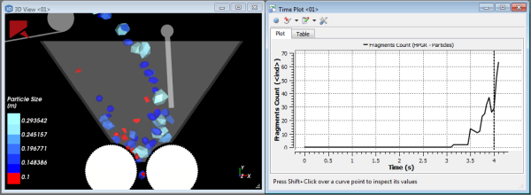
It is important to realize that breakage data is only collected after the Breakage Start value on the Solver | Time tab is reached. This is to allow enough time for the particle flow within your simulation to reach a steady state before breakage calculations begin.
For further details on the specific models, tips, and limitations see the About Particle Breakage topic.
Set up your simulation as you normally would (see also Set Simulation Parameters), ensuring all of the following:
During the Set Simulation-Wide Parameters step, on the Solver | Time tab, you have set the values you want for both Breakage Start and Breakage Delay after Release. (See also About Solver Parameters.) Tip: It is best practice to set your Breakage Start time to begin after a steady state has been reached for your particle flow.
During the Add and Edit Particle Sets step, you have done all of the following for each of the |Gloss7|s you want breakage enabled:
On the Particle tab, you have ensured that one of the following Shape | Composition option combinations are selected:
Either Straight or Custom Fiber Shape | Multiple Element Composition
Custom Shell Shape | Multiple Element Composition
Solid Polyhedron Shape | either Single Element or Multiple Element Composition
Solid Briquette Shape | Single Element Composition
Solid Faceted Cylinder Shape | Single Element Composition
Solid Custom Convex Polyhedron Shape | either Single Element or Multiple Element Composition
Solid Custom Concave Polyhedron Shape| Multiple Element Composition
If you have selected a Single Element particle set, you have done all of the following:
On the Particle | Breakage tab, you have selected the Enable Breakage checkbox.
From the Criteria sub-tab, you have selected the Instantaneous Breakage model you want from the Model list, and have defined its associated parameters.
From the Fragments sub-tab, you have entered the values you want under Limits, have chosen the model you want from the Distribution model list, and have defined its associated parameters.
If you have selected a Multiple Element particle set, you have done all of the following:
On the Particle | Breakage tab, you have selected the Discrete Breakage model you want from the Model list.
You have defined the model's associated parameters.
Process your simulation as you normally would. (See also About Starting a Simulation.)
After your simulation reaches as least as far as the Breakage Start time, do one or more of the following:
From a 3D View window (see also About 3D View Windows), observe the changes to the particle shapes as they fragment and break.
From the Data panel, select Particles and then from the Data Editors panel, select either the Properties or Curves tab and then create a plot (see also Graph Data within Rocky by Creating a Plot or Histogram) or visualize the resulting fragments-related Properties in a 3D View window (see also About 3D View Windows).
See Also:
CREATE AND VIEW A PARTICLE ASSEMBLY
(See also About Particle Assemblies.)
To Create and View a Particle Assembly:
Begin setting up your simulation as you normally would (see also Set Simulation Parameters).
During the Add and Edit Particle Sets step, do the following:
For each part you want represented in your final Assembly shape, create an individual Particle set. (See also Add a New Particle Set.) Tip: Ensure your Particle set meets the specific criteria for Assembly parts. (Refer to the Assembly Particle Shape Limitations section of the Particle and Input Limitations topic for details.)
Create another new Particle set (see also Add a New Particle Set), select it, and then from the Data Editors panel, do the following:
From the main Particle tab, define the Shape as an Assembly.
From the Shape sub-tab, add a new definition row for each individual part you want to include, and define each's part's position, size scale, and rotation parameters. (See also About Adding and Editing Particle Sets.) Tip: Check your settings in the Particles Details window. (About Particles Details Windows.) Note: For Assembly shapes, the Particles Details 3D view shows the actual position of the part when the size type is Original Size Scale and it is set to 1 (which is the default setting).
Define the rest of the shape settings as you normally would for any other Particle set. (Define what parameters you want on the Size, Movement, and Orientation sub-tabs.) Important:At this point, Rocky will calculate the mass, area, and other properties for the (whole) Assembly particle based on the values you have defined for the Particle sets upon which the individual parts are based, and the size of the parts you have defined within the Assembly. These properties will be calculated accurately by Rocky as long as your individual parts do not overlap; otherwise, the accuracy of these Rocky-calculated properties cannot be guaranteed and you should consider defining them yourself by specifying Custom Properties.
(Optional) If your Assembly shape requires its parts to overlap, and you require accurate mass, area, and other properties for your Assembly particle, consider specifying Custom Properties for your assembly by doing the following:
From the CAD program with which you designed your ideal (Assembly) particle shape, note the Area, Volume, Mass, Geometric Center, Center of Mass, and other properties you want Rocky to use for your Assembly particle shape.
In Rocky, from your Assembly particle's Particle | Custom Properties tab, enable the Change Assembly Properties checkbox, and then enter the information you want Rocky to use. Tip: You can use the colored dots in the Particles Details window to preview where your Center of Mass (blue dot) and Geometric Center (yellow dot) are located.
Finish setting up your simulation, process it, and then analyze the results as you normally would.
See Also:
ENABLE THERMAL MODELING CALCULATIONS
If you want to observe how particles are affected by temperature changes brought on by the heating or cooling of other items around it, you may set up your simulation to model thermal properties. Turning on Thermal Modeling enables you to simulate conductive heat transfer from particles to other particles, and from particles to boundaries. When used with CFD Coupling methods, it can also simulate convective heat transfer between particles and fluids. (See also Set or Modify Fluid and/or Air Flow Properties.)
Tip: For examples and walk-through tutorials of thermal modeling in action, review the following resources:
To enable Thermal Modeling in DEM calculations:
Set up your simulation as you normally would (see also Set Simulation Parameters), ensuring all of the following:
During the Set Simulation-Wide Parameters step, on the Physics tab, select the Enable Thermal checkbox. (See also About Physics Parameters.) Note: If you decide to enable Intra-particle Collision Statistics, know that the Temperature property will not be available to view on the Particles Details window, but can still be viewed from the main Particles entity or through a 3D View window. (Se also About Intra-Particle Collision Statistics.)
During the Add and Edit Geometry Components step, on the Geometry sub-tab for each of your wall components, set what you want for Thermal Boundary Type and Temperature.
During the Add and Edit Particle Sets step, on the Particle tab for the Particle set(s) you want affected by Thermal, ensure that on the Composition sub-tab for any particles you have you have selected Multiple Elements from the Composition list, that you also set the Conductivity Ratio parameter to the value you want.
During the Modify Material Properties step, on the Materials tab for each of your particle and/or boundary materials, set all of the following parameters:
Thermal Conductivity
Specific Heat
Poisson's ratio (See also About Modifying Material Compositions.)
During the Add and Edit Particle Inputs step, for each Particle Input, set the Temperature of each Particle set row. (See also About Adding and Editing Particle Inputs.)
If coupling your simulation with CFD methods, then during the Set or Modify Fluid and/or Air Flow Properties step, set what you want for the Convective Heat Transfer Law. (See also About Using the 1-Way Fluent Method, About Using the 2-Way Fluent Method, or About Using the 1-Way Constant Method). Note: If coupling your simulation with the 1-Way Constant method specifically, ensure you also set the values you want for constant Temperature, Thermal Conductivity, and Specific Heat. (See also About Using the 1-Way Constant Method.)
Process your simulation as you normally would. (See also About Starting a Simulation.)
To enable Thermal Modeling in SPH calculations:
Set up your simulation as you normally would (see also About SPH Parameters), ensuring all of the following:
During the Set Simulation-Wide Parameters step, on the Physics tab, select the Enable Thermal checkbox. (See also About Physics Parameters.) The Cleary model for thermal transfer is automatically selected.
During the Add and Edit Geometry Components step, on the Geometry sub-tab for each of your wall components, set what you want for Thermal Boundary Type and Temperature.
If you simulation also involves DEM particles: During the Add and Edit Particle Sets step, on the Particle tab for the Particle set(s) you want affected by Thermal, ensure that on the Composition sub-tab for any particles you have you have selected Multiple Elements from the Composition list, that you also set the Conductivity Ratio parameter to the value you want.
During the Modify Material Properties step, on the Materials tab set all of the following parameters for the fluid material:
Thermal Conductivity
Specific Heat
Process your simulation as you normally would. (See also About Starting a Simulation.)
Tip: When you are ready to analyze your simulation (see also Analyzing a Simulation), you might pay special attention to the following Properties (see also About Properties):
Temperature (for walls, conveyors, particles and fluids)
Specific Heat (only for fluids)
Thermal Conductivity (only for fluids)
See Also:
A 3D View of your simulation will always contain the Rocky logo but you can choose to add your own company logo to the view, too. This may be useful in cases where you are showing simulation images or animations to clients and want to brand your work.
You add a logo image by using the Overlay tab on the Window Editors panel. Logos are added as images and can be positioned anywhere on the 3D View window that you like.
Using separate image editing software, open the logo file you want to use and ensure the display size is appropriate.
Ensure your image is saved as either a PNG, JPG, BMP, or PNP file.
Open the simulation project to which you want to add the logo and select the 3D View window you want.
Using the Overlay tab on the Window Editors panel, add the logo to the 3D View as an Image Overlay. (See also Add or Edit an Image Overlay for a 3D View Window.)
See Also:
REUSE 3D VIEW WINDOW, WORKSPACE, AND USER PROCESS SETUPS IN OTHER PROJECTS
For projects where you have spent time and effort setting up several 3D View windows, Workspaces, and User Processes just the way you like, you can now export all of that setup criteria and reuse it in other projects. This is an alternative to recording or writing a script to do the setup for you, which requires you to know beforehand exactly how you want your views and processes to work. With this feature, you can decide after the fact whether you want to reuse the setup for another project or not.
This can be useful in cases where you have already run several similar simulations but your client suddenly wants to see new views or processes. By using this feature, you can set up the new views and processes in one project, and then apply those same views and processes to the rest of the projects in your set.
Rocky enables you to export this setup criteria to either a
rocky_template file or to the clipboard, and even lists each
component that was exported in a separate dialog (Figure 1) for confirmation
purposes.
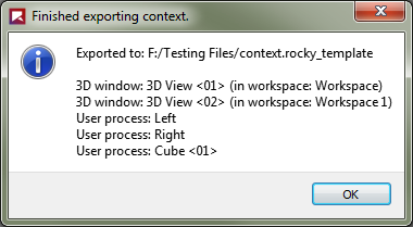 Example dialog that appears after exporting
project context
Example dialog that appears after exporting
project context
In your new project, you can then choose to import the saved criteria from those same two locations.
Once imported, Rocky simply creates new 3D View windows, Workspaces, and User Processes to match what was exported. If you already have 3D View windows and User Processes in your project at the time of Import, Rocky will retain these items while adding the new ones to the project.
To export 3D View window, Workspace, and User Process setups for use in other projects:
Ensure that your 3D View windows, Workspaces, and User Processes are set up the way you want.
From the File menu, point to Export project context and then do one of the following:
To ensure reuse of the project context for longer than just the immediate timeframe, select To file, and then do all of the following: a. From the Save project context dialog, select the location to which you want to save the
rocky_templatefile, name it in the File name box, and then click Save. b. In the Finished exporting context dialog, review the items listed, and then click OK.To reuse the project context for only the immediate timeframe, select To clipboard, and then in the Finished exporting context dialog, review the items listed, and then click OK.
The 3D Window, Workspace, and User Process setups are ready to import into another project.
To import 3D View window, Workspace, and User Process setups previously exported out of another project
Ensure the project that you want to apply the previously exported setups is open in Rocky.
From the File menu, point to Import project context and then do one of the following:
To import from a previously exported file, select From file, and then from the Restore project context dialog, locate and select the
rocky_templatefile you want to use, and then click Open.To import from the clipboard, select From clipboard.
The 3D Window, Workspace, and User Process setups you previously exported are added to the project.
See Also:
When setting up a new GPU card for use with Rocky, there are two steps you can take that might help make processing your simulations on GPU smoother and faster:
Turn off the Windows Timeout Detection and Recovery (TDR)
Enable double-precision processing
See below for specific instructions.
Turn off Timeout Detection and Recovery (TDR) for a GPU card
Application: This procedure is particularly useful when you have a single NVIDIA GPU card. But it can also be useful for any GPUs used by Rocky in general.
Symptom: Your Rocky simulations sporadically stop during the middle of a complex simulation, resulting in an incomplete calculation and an error (Figure 1). This is caused by Windows believing the GPU card is non-responsive because it is taking longer than expected to return an answer on a difficult calculation. Turning off TDR for your GPU allows the card the necessary time to execute the computation.
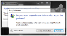
To turn off TDR for a GPU card:
Ensure that you have successfully installed your GPU card and associated drivers, and have restarted your computer.
Download and install the latest NVIDIA Nsight Visual Studio Edition from Nvidia.
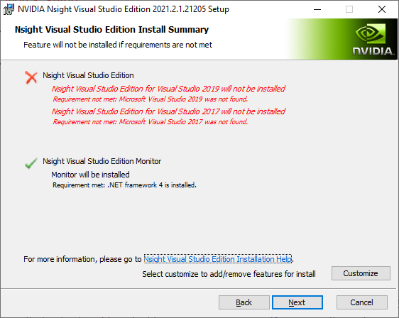 Figure 2: Installation confirmation screen
for Nsight Visual Studio Edition
Figure 2: Installation confirmation screen
for Nsight Visual Studio Edition Notes:
As seen in Figure 2 above, you will need only to install the Nsight Monitor option; the Nsight Visual Studio option is not necessary.
You may need to Subscribe as a developer (free of charge) on the Nvidia website, if you haven't done it before, in order to download the Nsight Visual Studio Edition (Figure 3).
 Figure 3: Subscribe to Nvidia developer
program
Figure 3: Subscribe to Nvidia developer
program Restart your computer.
From the Windows Start menu, under NVIDIA Corporation, click Nsight Monitor (Figure 4).
 Figure 4 Nsight Monitor in Windows Start
menu A new Nsight Monitor icon appears in
your Notification Area.
Figure 4 Nsight Monitor in Windows Start
menu A new Nsight Monitor icon appears in
your Notification Area.From your Notification Area, right-click the Nsight Monitor icon and then select Options (Figure 5).
 Figure 5: Nsight Monitor in Notification
Area
Figure 5: Nsight Monitor in Notification
AreaFrom the NVIDIA Nsight Options dialog, on the General tab, set WDDM TDR enabled to False (Figure 6).
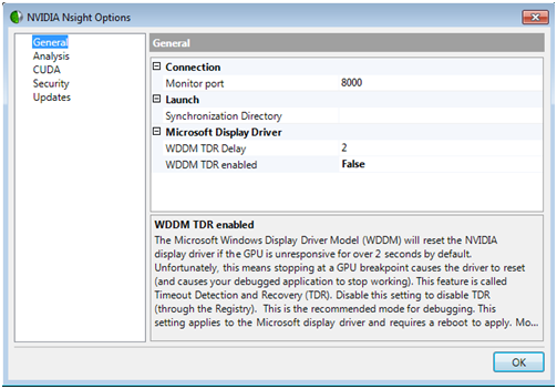 Figure 6: NVIDIA Nsight Options
dialog
Figure 6: NVIDIA Nsight Options
dialogClick OK.
Restart your computer.
Enable double-precision processing for your GPU cards
Application: You have one or more GPU cards from the NVIDIA Titan family.
Symptom: You are seeing slower than expected results on your Titan family GPU card. This could be a result of not yet enabling double-precision processing. Doing so will speed up certain Rocky calculations, thereby reducing your overall processing time, at the expense of slowing down your graphics visualization performance. Additionally, it has been found that a Titan card using double precision will take longer when simulating Spheres (~20%), but will be faster when simulating shaped particles (~200%).
To enable double-precision processing for your GPU cards:
Ensure that you have successfully installed your Titan card(s) and associated drivers, and have restarted your computer.
Right-click your Windows desktop, and then click NVIDIA Control Panel (Figure 7).
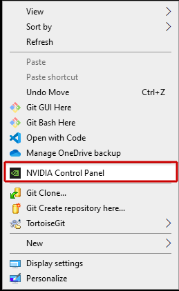 Figure 7: Windows desktop right-click menu
showing NVIDIA Control Panel option
Figure 7: Windows desktop right-click menu
showing NVIDIA Control Panel optionIn the NVIDIA Control Panel window, do all of the following:
From the Select a Task list, select Manage 3D settings.
In the Global Settings tab under Feature, select Double precision and then from the drop-down list, ensure all your Titan GPU cards are enabled (checked) (Figure 8).
 Figure 8: Manage 3D Settings section in
the NVIDIA Control Panel
Figure 8: Manage 3D Settings section in
the NVIDIA Control PanelClick OK.
Restart your computer.
See Also: