From the Toolbox, drag a Rigid Dynamics template to the Project Schematic.

Density is the only material property utilized by rigid bodies. Models that use zero or nearly zero density fail to solve with the Ansys Rigid Dynamics solver.

Sheet, solid, and line bodies are supported by the Ansys Rigid Dynamics solver, but line bodies can only be flexible and included in a condensed part. Plane bodies cannot be used.

Rigid line bodies are not supported in RBD because the mass moment of inertia is not available.

You can define a Point Mass for this analysis type.

Stiffness behavior can be rigid or flexible.

---

Note:  If the part behavior is flexible, it must be included in a condensed part.

---

Applicable connections are joints, springs, and contacts.

When an assembly is imported from a CAD system, joints or constraints are not imported, but joints may be created automatically after the model is imported. You can also choose to create the joints manually.

Each joint is defined by its coordinate system of reference. The orientation of this coordinate system is essential as the free and fixed degrees of freedom are defined in this coordinate system.

Automatic contact generation is also available after the model is imported.

For information on contact specifically oriented for Rigid Dynamics, see Contact in Rigid Dynamics and Best Practices for Contact in Rigid Body Analyses.

Mesh controls apply to surfaces where contact is defined as well as to deformable parts.

For Rigid Dynamics analyses the basic controls are:

Step Controls enable you to create multiple steps. Multiple steps are useful if new loads are introduced or removed at different times in the load history.

A Rigid Dynamics analysis can use an explicit time integration scheme, especially if the model is made only of rigid parts. Unlike the implicit time integration, there are no iterations to converge in an explicit time integration scheme. The solution at the end of the time step is a function of the derivatives during the time step. As a consequence, the time step required to get accurate results is usually smaller than is necessary for an implicit time integration scheme. Another consequence is that the time step is governed by the highest frequency of the system. A very smooth and slow model that has a very stiff spring will require the time step needed for the stiff spring itself, which generates the high frequencies that will govern the required time step. Stiff models can be more efficiently solved using the Implicit Generalized-α, Implicit Stabilized Generalized-α, or MJ Time Stepping time integration schemes.

Because it is not easy to determine the frequency content of the system, an automatic time stepping algorithm is available, and should be used for the vast majority of models. This automatic time stepping algorithm is governed by Initial Time Step, Minimum Time Step, and Maximum Time Step under Step Controls; and Energy Accuracy Tolerance under Nonlinear Controls.

• Initial Time Step: If the initial time step chosen is vastly too large, the solution will typically fail, and produce an error message that the accelerations are too high. If the initial time step is only slightly too large, the solver will realize that the first time steps are inaccurate, automatically decrement the time step and start the transient solution over. Conversely, if the chosen initial time step is excessively small, and the simulation can be accurately performed with higher time steps, the automatic time stepping algorithm will, after a few gradual increases, find the appropriate time step value. Choosing a good initial time step is a way to reduce the cost of having the solver figure out what time step size is optimal to minimize run time. While important, choosing the correct initial time step typically does not have a large influence on the total solution time due to the efficiency of the automatic time stepping algorithm.

• Minimum Time Step: During the automatic adjustment of the time step, if the time step that is required for stability and accuracy is smaller than the specified minimum time step, the solution will not proceed. This value does not influence solution time or its accuracy, but it is there to prevent the solver from running forever with an extremely small time step. When the solution is aborting due to hitting this lower time step threshold, that usually means that the system is over constrained, or in a lock position. Check your model, and if you believe that the model and the loads are valid, you can decrease this value by one or two orders of magnitude and run again. That can, however generate a very large number of total time steps, and it is recommended that you use the Output Controls settings to store only some of the generated results.

• Maximum Time Step: Sometimes the time step that the automatic time stepping settles on produces too few results outputs for precise postprocessing needs. To avoid these postprocessing resolution issues, you can force the solution to use time steps that are no bigger than this parameter value.

Solver Controls: For this analysis type, enables you to select a time integration algorithm (Program Controlled, Runge-Kutta order 4, Implicit Generalized-α, Stabilized Generalized-α, MJ Time Stepping) and select whether to use constraint stabilization. The default time integration option, Program Controlled, provides the appropriate accuracy for most applications. The default, Program Controlled is valid for most applications, however; you may wish to set this option to User Defined and manually enter customized settings for weak spring and damping effects. The default is Off.

Nonlinear Controls enable you to modify convergence criteria and other specialized solution controls. Typically you will not need to change the default values for this control.

• Energy Accuracy Tolerance: This is the main driver to the automatic time stepping. The automatic time stepping algorithm measures the portion of potential and kinetic energy that is contained in the highest order terms of the time integration scheme, and computes the ratio of the energy to the energy variations over the previous time steps. Comparing the ratio to the Energy Accuracy Tolerance, Workbench will decide to increase or decrease the time step. Energy accuracy tolerance is program controlled by default. It is enabled with the Explicit Runge-Kutta method and disabled by default with Implicit Generalized-α, Implicit Stabilized Generalized-α, and MJ Time Stepping.

  ---

  Note:  For systems that have very heavy slow moving parts, and also have small fast moving parts, the portion of the energy contained in the small parts is not dominant and therefore will not control the time step. It is recommended that you use a smaller value of integration accuracy for the motion of the small parts.

  Spherical, slot and general joints with three rotation degrees of freedom usually require a small time step, as the energy is varying in a very nonlinear manner with the rotation degrees of freedom.

  ---

• Force Residual Relative Tolerance: (Only available with Implicit Generalized-α or Stabilized Generalized-α time integration or MJ Time Stepping integration) This option controls the threshold used in Newton-Raphson for force residual convergence. The default value is 1.e-7. A smaller value will lead to a smaller residual, but it will require more iterations. The convergence of force residual can be monitored in Solution Information using Force Convergence.

• Constraint Equation Residual Relative Tolerance: (Only available with Implicit Generalized-α or Stabilized Generalized-α time integration or MJ Time-Stepping integration) This option controls the threshold used in Newtom-Raphson to check convergence of constraint equations violations. The default value is 1.e-8. The convergence of this criterion can be checked in Solution Information using Displacement Convergence

Output Controls enable you to specify the time points at which results should be available for postprocessing. In a transient nonlinear analysis it may be necessary to perform many solutions at intermediate time values. However i) you may not be interested in reviewing all of the intermediate results and ii) writing all the results can make the results file size unwieldy. This group can be modified on a per step basis.

Before solving, you can configure the joints and/or set a joint load to define initial conditions.

1. Define a Joint Load during a short initial load step to set initial conditions on the free degrees of freedom of a joint.

   For the Ansys Mechanical APDL solver to converge, it is recommended that you ramp the angles and positions from zero to the real initial condition over one step. The Ansys Rigid Dynamics solver does not need these to be ramped. For example, you can directly create a joint load for a revolute joint of 30 degrees, over a short step to define the initial conditions of the simulation. If you decide to ramp it, you have to keep in mind that ramping the angle over 1 second, for example, means that you will have a non-zero angular velocity at the end of this step. If you want to ramp the angle and start at rest, use an extra step maintaining this angle constant for a reasonable period of time or, preferably, having the angular velocity set to zero. Another way to specify the initial conditions in terms of positions and angles is to use the Configure tool, which eliminates the time steps needed to apply the initial conditions.

   To fully define the initial conditions, you must define position and velocities. Unless specified by joint loads, if your system is initially assembled, the initial configuration will be unchanged. If the system is not initially assembled, the initial configuration will be the "closest" configuration to the unassembled configuration that satisfies the assembly tolerance and the joint loads.

   Unless specified otherwise, relative joint velocity is, if possible, set to zero. For example, if you define a double pendulum and specify the angular velocity of the grounded revolute joint, by default the second pendulum will not be at rest, but will move rigidly with the first one.

2. Configure a joint to graphically put the joint in its initial position.

See Joint Initial Conditions for further details.

The following loads and supports can be used in a Rigid Dynamics analysis:

• Acceleration

• Standard Earth Gravity

• Joint Load

• Remote Displacement

• Remote Force

• Constraint Equation

Joint Load

Magnitude

For a Joint Load, the joint condition's magnitude could be a constant value, could vary with time as defined in a table or via a function, or could depend on other values measured on the model during the solution. See Using the Variable Load Add-on to define such a load variation. Details of how to apply a tabular or function load are described in Specifying Boundary Condition Magnitude. Details on the Joint Load are included below.

In addition, for more information about time stepping and ramped loads, see the Applying Stepped and Ramped Loads section.

Interpolation/Derivation

For joint loads applied through tabular data values, the number of points input will most likely be less than the number of time steps required to solve the system. As such, an interpolation is performed. When a joint load requires fitting, the result of the fitting is displayed in the joint load chart along with the user-specified values. The number of segments used to display the curve is driven by the Number Of Segments property.

The underlying fitting method used for interpolation can be configured using the Fitting Method field (specific to Rigid Dynamics analysis). Options include:

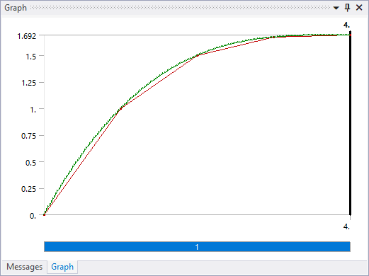
• Program Controlled (default): Depending on the Joint Load type, the solver chooses the appropriate interpolation method. Accelerations and Force joint loads use a piecewise linear. Displacement/Rotation/Velocity/Rotational Velocity joint loads use either a linear fitting when only two points are given per load step, or a cubic spline fitting when there are more than two points as shown on the following graph:

  

  A large difference between the interpolated curve and the linear interpolation may prevent the solution from completing. If this is the case and you intend to use the linear interpolation, you can simply use multiple time steps, as the interpolation is done in one time step.

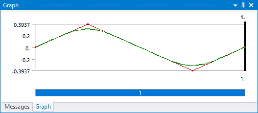
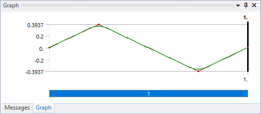
• Fast Fourier Transform: Fast Fourier Transform is performed to fit tabular data. Unlike cubic spline fitting, no verification on the fitting quality is performed. The additional cutoff frequency parameter specifies the threshold (expressed in Hz) used to filter high frequencies. Higher cutoff frequency results in a better fitting, but leads to smaller time steps. The following graphs show the effect of cutoff frequency on FFT fitting on a triangular signal using 5 Hz and 10 Hz, respectively.

  ---

  Note:  The Fourier Fitting implicitly expects cyclic data. Lack of continuity between end time and start time values may lead to oscillations known as Gibbs phenomenon. Similarly, the lack of continuity for the derivatives may also lead to unwanted oscillations around jumps. For instance, an imposed displacement requires the continuity of the first and second derivatives. The Rigid Dynamics solver implements several dedicated treatments to prevent Gibbs phenomenon. However, results of Fourier Fitting must be carefully reviewed to check there are no artificial oscillations.

  ---

  
  

Discontinuities

When defining a joint load for a position and an angle, the corresponding velocities and accelerations are computed internally. When defining a joint load for a translational and angular velocity, corresponding accelerations are also computed internally. By activating and deactivating joint loads, you can generate some forces/accelerations/velocities, as well as position discontinuities. Always consider what the implications of these discontinuities are for velocities and accelerations. Force and acceleration discontinuities are perfectly valid physical situations. No special attention is required to define these velocity discontinuities. Discontinuities can be obtained by changing the slope of a relative displacement joint load on a translational joint, as shown on the following graphs using two time steps:

The corresponding velocity profile is shown here.

This discontinuity of velocity is physically equivalent to a shock, and implies infinite acceleration if the change of slope is over a zero time duration. The Ansys Rigid Dynamics solver will very often handle these discontinuities, and redistribute velocities after the discontinuity according to all active joint loads. This process of redistribution of velocities usually provides accurate results; however, no shock solution is performed, and this process is not guaranteed to produce a physically acceptable energy redistribution. A closer look at the total energy probe will tell you if the solution is valid. In case the redistribution is not done properly, use one step instead of two to use an interpolated, smooth position variation with respect to time.

Discontinuities of positions and angles are not a physically acceptable situation. Results obtained in this case may not be physically sensible. Workbench cannot detect this situation up front. If you proceed with position discontinuities, the solution may abort or produce false results.

Rotations

For fixed axis rotations, it is possible to count a number of turns. For 3D general rotations, it is not possible to count turns. In a single axis case, although it is possible to prescribe angles higher than 2π, it is not recommended because Workbench can lose count of the number of turns based on the way you ramp the angle. You should avoid prescribing angular displacements with angles greater than Pi when loading bushing joints, because the angle-moment relationship could differ from the stiffness definition if the number of turns is inaccurate, or in case of Euler angles singularity. It is highly recommended that you use an angular velocity joint load instead of an angle value to ramp a rotation, whenever possible.

For example, replace a rotation joint load designed to create a joint rotation from an angle from 0 to 720 degrees over 2 seconds by an angular velocity of 360 degrees/second. The second solution will always provide the right result, while the behavior of the first case can sometimes lead to the problems mentioned above.

For 3D rotations on a general joint for example, no angle over 2π can be handled. Use an angular velocity joint load instead.

Multiple Joint Loads On The Same Joint

When prescribing a position or an angle on a joint, velocities and acceleration are also prescribed. The use of multiple joint loads on the same joint motion can cause for joint loads to be determined inaccurately.

Only synchronous solves are supported for Rigid Dynamics analyses.

Use a Solution Information object to track, monitor, or diagnose problems that arise during solution.

Applicable results are Deformation and Probe results.

---

Note:  If you highlight Deformation results in the tree that are scoped to rigid bodies, the corresponding rigid bodies in the Geometry window are not highlighted.

---

To plot different results against time on the same graph or plot one result quantity against a load or another results item, use the Chart and Table feature.

If you duplicate a Rigid Dynamics analysis, the results of the duplicated branch are also cleared.