


A joint typically serves as a junction where bodies are joined together. Joint types are characterized as fixed or free depending on their rotational and translational degrees of freedom. If you specify a Joint as a it is classified as a remote boundary condition. Refer to the Remote Boundary Conditions section for a listing of all remote boundary conditions and their characteristics.
The section includes the following joint characteristics:
Supported Analysis Types
Joints are supported in the following structural analyses:
Note:
A joint cannot be applied to a vertex scoped to an end release.
When you set the property to , the application uses the element COMBI250. As a result:
The Element Coordinate System is the first coordinate system used to apply rotation.
This is followed by nodal rotations defined on associated Remote Points (Reference or Mobile), such as the NROTAT command that rotates nodal coordinate systems into the active system. In addition, rotations from these remote points modify the element matrix (see the Input Data topic of the COMBI250 element reference).
This is then followed by the normal processing sequence for rotations.
Ansys recommends that you specify the same coordinate system for Element Coordinate System, Reference Coordinate System, and Mobile Coordinate System properties in case there is a relative rotation between the Element Coordinate System and either the Reference Coordinate System or Mobile Coordinate System. In addition, you need to verify proper rotation as well as results.
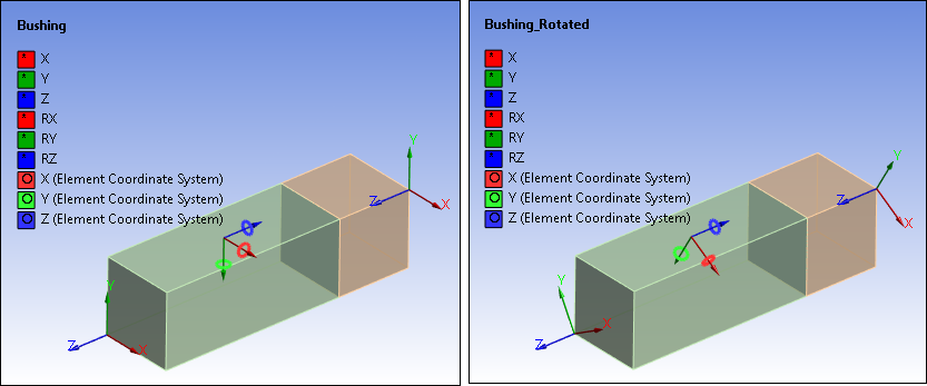
Here is an example of Element Coordinate System annotations ("rings" about each axis), prior to and after rotation.
Each multibody part made of rigid bodies is treated as a single, rigid part. Consequently, joints must not be created within a multibody part.
Similarly, functionalities such as configure, assemble, model topology, or redundancy analysis always consider each multibody part as a single part, regardless stiffness behavior. Joints must be defined between independent parts or multibody parts to use these functionalities.
The Samcef Solver interface supports all joint types except for the fixed joint, slot joint, and the imperfect joints. Only supported joint types are active in the Mechanical interface.
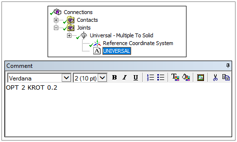
To maintain consistency with the characteristics of Samcef joints, you must insert a Comment object with the correct name under the joint object. The comment permits you to capture joint properties which are not available in the view in Mechanical. The comment functions similarly to a commands object: the content of the comment is appended to the description of the joint in the solver input file. The necessary name for the comment object is listed for each joint type.
Nature of Joint Degrees of Freedom
For all joints that have both translational degrees of freedom and rotational degrees of freedom, the kinematics of the joint are defined such that the moving coordinate system translates in the reference coordinate system. For example, if a joint is a slot, the translation along X is expressed in the reference coordinate system.
Once the translation has been applied, the center of the rotation is the location of the moving coordinate system.
For the Mechanical APDL solver, the relative angular positions for the spherical, general, and bushing joints are characterized by the Cardan (or Bryant) angles. This requires that the rotations about the local Y axis be restricted between -π/2 to +π/2. Therefore, the local Y axis should not be used to simulate the axis of rotation if the expected rotation is large.
Joint Abstraction
Joints are considered as point-to-point in the solution though the user interface shows the actual geometry. Due to this abstraction to a point-to-point joint, geometry interference and overlap between the two parts linked by the joint can be seen during an animation.
When using the Ansys Explicit Dynamics solver the contact algorithm will be active for the mesh by default. This means that free DOF's may be restrained by contact forces.
Joint Initial Conditions
The degrees of freedom are determined depending on the selected solver. For the Ansys Rigid Dynamics solver, the degrees of freedom are the relative motion between the parts. For the Ansys Mechanical solver and the Ansys Explicit Dynamics solver, the degrees of freedom are the location and orientation of the center of mass of the bodies.
When initial conditions are applied, there are two means for the Ansys Rigid Dynamics solver to initialize the velocities:
A pure kinematic method, only based on the kinematic constraints. It minimizes the position and velocity increments.
A method using the inertia matrix. The position increment, scaled by the inertia matrix, is minimized; while the velocity increment is calculated in order to minimize the kinetic energy.
Unless otherwise specified using joint conditions, the Mechanical APDL solver, Ansys Rigid Dynamics solver, and Ansys Explicit Dynamics solver start with initial velocities equal to zero. This has different implications for the solvers. For the Mechanical APDL solver and the Ansys Explicit Dynamics solver, this means that the bodies will be at rest. For the Ansys Rigid Dynamics solver, this means that the relative velocities will be at rest.
Consider, for example, an in-plane double pendulum, with a constant velocity specified for the first grounded link. The two solvers will treat this scenario as follows:
Using the Ansys Rigid Dynamics solver:
If the first method is used, the second link has the same rotational velocity as the first, because the relative velocity is initially equal to zero.
If the second method is used, the second link does not start with the same initial velocity as the first link.
Using the Mechanical APDL solver or the Ansys Explicit Dynamics solver, the second link starts at rest.
Joint DOF Zero Value Conventions
Joints can be defined using one or two coordinate systems: the Reference Coordinate System and the Mobile Coordinate System.
The use of two coordinate systems can be beneficial in certain situations, such as when a CAD model is not imported in an assembled configuration. Using two coordinate systems also enables you to employ the and features (see Manual Joint Creation), and it gives you the ability to update a model following a CAD update.
For the Ansys Rigid Dynamics solver, the zero value of the degrees of freedom corresponds to the matching reference coordinate system and moving coordinate system.
If a joint definition includes only the location of the Reference Coordinate System (see Modifying Joint Coordinate Systems), then the DOF of this joint are initially equal to zero for the geometrical configuration where the joints have been built.
If the Mobile Coordinate System is defined using the Override option, then the initial value of the degrees of freedom can be a nonzero value.
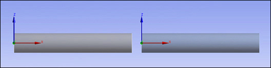
Consider the example illustrated below. If a Translational joint is defined between the two parts using two coordinate systems, then the distance along the X axis between the two origins is the joint initial DOF value. For this example, assume the joint initial DOF value is 65 mm.
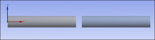
Conversely, if the joint is defined using a single coordinate as shown below, then the same geometrical configuration has a joint degree of freedom that is equal to zero.
For the Mechanical APDL solver and the Ansys Explicit Dynamics solver, having one or two coordinate systems has no affect. The initial configuration corresponds to the zero value of the degrees of freedom.
Joint Condition Considerations
When applying a Joint Condition, behavior varies depending on the solver selected. The following tables demonstrate variations in solver behavior, using the right part of the translational joint illustrated above moving 100 mm towards the other part over a 1 second period. (The distance along the X axis is 65 mm.)
| Solver | Displacement Joint Condition | |
| Time | Displacement | |
| Ansys Rigid Dynamics – Two Coordinate Systems | 0 | 65 |
| 1 | 165 | |
| Ansys Rigid Dynamics – One Coordinate System | 0 | 0 |
| 1 | 100 | |
| Mechanical APDL, Ansys Explicit Dynamics – Two Coordinate Systems | 0 | 0 |
| 1 | 100 | |
| Mechanical APDL, Ansys Explicit Dynamics – One Coordinate System | 0 | 0 |
| 1 | 100 | |
You can unify the joint condition input by using a Velocity Joint Condition.
| Solver | Velocity Joint Condition | |
| Time | Velocity | |
| – Two Coordinate Systems | 0 | 100 |
| 1 | 100 | |
| – One Coordinate System | 0 | 100 |
| 1 | 100 | |
| – Two Coordinate Systems | 0 | 100 |
| 1 | 100 | |
| – One Coordinate System | 0 | 100 |
| 1 | 100 | |