


You use the Step Controls category during static and transient dynamic analyses to first specify a multiple step analysis, and then define all associated properties, including those of the Nonlinear Controls and Output Controls, for each step.
Go to a section topic:
Specifying Step Controls
The Step Controls category of the Analysis Settings object includes the properties described below. The display of certain properties can depend upon the selections that you make, the type of analysis you are performing, as well as the use of a particular feature. Note that most Step Controls (as well as Nonlinear Controls and Output Controls) are “step aware,” that is, property settings can be different for each step.
- Number of Steps
Use this property to define the desired number of steps for your analysis. The Graph and Tabular Data windows automatically update with the specified number of steps.

- Current Step Number
This property displays the currently selected step. The default setting is
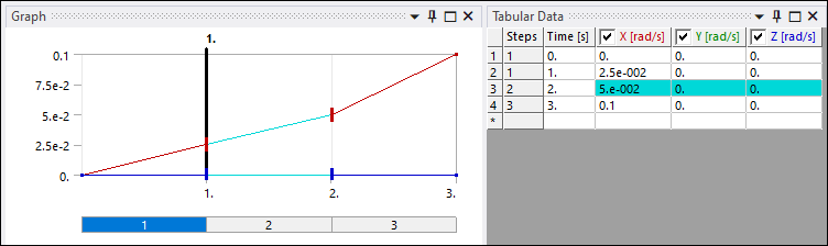
1. To select a particular step, you can 1) change the value of this property, 2) select a time value in the Graph window (or the step bar displayed below the chart), or 3) select a row in the Step column of the Tabular Data window. When you change the value of this property, your entry is reflected in the Graph and Tabular Data windows. An example is illustrated below for a Current Step Number value of2.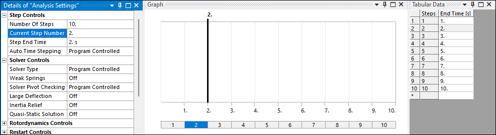
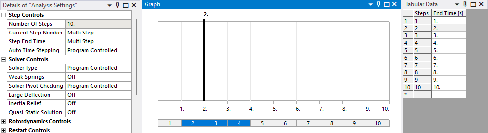
You can select multiple steps in the Graph window using the [Shift] and [Ctrl] keys. When you select multiple steps, the Current Step Number property displays the value Multi Step. For this type of selection, any changes affect all of the selected steps.
Note: The selection of multiple steps is not supported for an Explicit Dynamics or a Rigid Body Dynamics analysis. If multiple steps are highlighted in the Graph window and changes made to the Analysis Settings, the changes will affect the last selected step only.
- Step End Time
This property displays the end time of the Current Step Number. When multiple steps are selected this property displays the value Multi Step.
- Auto Time Stepping
Automatic time stepping is available for static and transient analyses, and is especially useful for nonlinear solutions. This property is also described in detail in the Automatic Time Stepping section.
This property provides a drop-menu with the following options:
(default): The Mechanical application automatically switches time stepping on and off as needed. A check is performed on non-convergent patterns. The physics of the simulation is also taken into account. The settings are presented in the following table:
Auto Time Stepping Program Controlled Settings Analysis Type Initial Substeps Minimum Substeps Maximum Substeps Linear Static Structural 1 1 1 Nonlinear Static Structural 1 1 10 Linear Steady-State Thermal 1 1 10 Nonlinear Steady-State Thermal 1 1 10 Transient Thermal 100 10 1000 : You control time stepping by completing the following fields that only appear if you choose this option. No checks are performed on non-convergent patterns and the physics of the simulation is not taken into account.
Initial Substeps: Specifies the size of the first substep. The default is
1.Minimum Substeps: Specifies the minimum number of substeps to be taken (that is, the maximum time step size). The default is
1.Maximum Substeps: Specifies the maximum number of substeps to be taken (that is, the minimum time step size). The default is
10.
: No time stepping is enabled. You are prompted to enter the Number Of Substeps. The default is
1.
- Define By
This property displays when you set the Auto Time Stepping property to or . Its drop-down menu contains the options and . The default setting for this property depends upon the analysis type. It enables you to set the limits on load increment in one of two ways. You can specify the Initial Time Step, Minimum Time Step and Maximum Time Step number of substeps for a step or equivalently specify the Time Substeps, Minimum Substeps and Maximum Substeps time step size.
- Carry Over Time Step
This property is available when you specify multiple steps. This is useful when you do not want any abrupt changes in the load increments between steps. When this is set to On, the Initial time step size of a step will be equal to the last time step size of the previous step.
- Time Step
This property displays a time value for the current step.
- Time Integration
This property is only available for Coupled Field Transient, Transient Structural, or Transient Thermal analyses. This field indicates whether a step should include transient effects, such as structural inertia or thermal capacitance, or whether it is a static (steady-state) step. This field can be used to set up the Initial Conditions for a transient analysis.
On: Default setting for transient analyses.
Off: This option does not include structural inertia or thermal capacitance in solving this step.
For a Coupled Field Transient analysis when the Time Integration property is set to , the following additional properties display and enable you to specify whether to turn a physics field on or off:
Structural Only: Options include (default) and .
Thermal Only: Options include and (default) .
Note: With Time Integration set to Off during Transient structural analyses, the application does not compute velocity results. Therefore spring damping forces, which are derived from velocity, will equal zero. This is not the case for Rigid Dynamics analyses.
Specify Settings for Multiple Substeps Simultaneously
If you want to specify the same analysis setting(s) to several substeps, you can select steps of interest as follows and change the analysis settings properties.
- Change All Steps
To specify analysis settings for all the substeps:
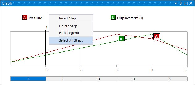
In either the Graph or Tabular Data window, right-click and select the option.

In the Details pane, make changes to properties. These changes will automatically apply to all steps.
- Change Multiple Steps from Graph Window
From the Graph window:
Highlight the Analysis Settings object.
Highlight steps in the Graph window using either of the following standard windowing techniques:
Ctrl key to highlight individual steps.
Shift key to highlight a continuous group of steps.
Specify the analysis settings as needed. These settings will apply to all selected steps.
- Change Multiple Steps from Tabular Data Window
From the Tabular Data window:
Highlight the Analysis Settings object.
Highlight steps in the Tabular Data window using either of the following standard windowing techniques:
Ctrl key to highlight individual steps.
Shift key to highlight a continuous group of steps.
Click the right mouse button in the window and choose from the context menu.
Specify the analysis settings as needed. These settings will apply to all selected steps.
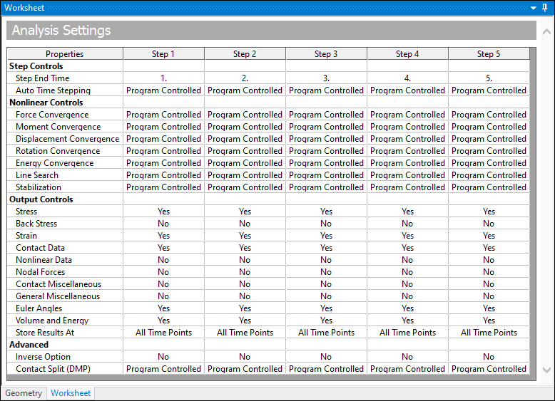
Display All Analysis Settings in the Worksheet
The Worksheet for the Analysis Settings object provides a single display of pertinent settings in the Details for all steps.
Note: For Explicit Dynamics, the Worksheet for the Analysis Settings object provides a single display of pertinent step-aware settings in the Details pane for all steps.
Activating and Deactivating Loads
You can activate (include) or deactivate (delete) a specified load from being used in the analysis within the time span of a step. For most loads, such as pressure or force, deleting the load is the same as setting the load value to zero. But for certain loads, such as a specified displacement, this is not the case.
Note:
Changing the method of how a multiple-step load value is specified (such as Tabular to Constant), the Activation/Deactivation state of all steps resets to the default, Active.
The activate/deactivate option is only available when the Independent Variable property or the X-Axis property is set to .
The capability to activate and/or deactivate loads is not available for the Samcef solver
To activate or deactivate a load in a stepped analysis:
Highlight the load within a step in the Graph or a specific step in the Tabular Data window.
Click the right mouse button and choose Activate/Deactivate at this step!.
Note: For displacements and remote displacements, it is possible to deactivate only one degree of freedom within a step.
Limitation: For a Mode Superposition Transient analysis, the application does not support deactivation of an Acceleration or a Displacement defined as a Base Excitation.
For Imported loads and Temperature, Thermal Condition, Heat Generation, Voltage, and Current loads, the following rules apply when multiple load objects of the same type exist on common geometry selections:
A load can assume any one of the following states during each load step:
Active: Load is active and data specified during the first step.
Reactivated: Load is active and data specified during the current step, but was deactivated during the previous step. A change in step status exists.
Deactivated: Load is deactivated at the current step, but was active and data applied during the previous step. A change in step status exists.
Unchanged: No change in step status exists.
During the first step, an active load will overwrite other active loads that exist higher (previously added) in the tree.
During any other subsequent step, commands are sent to the solver only if a change in step status exists for a load. Hence, any unchanged loads will get overwritten by other reactivated or deactivated loads irrespective of their location in the tree. A reactivated/deactivated load will overwrite other reactivated and deactivated loads that exist higher (previously added) in the tree.
Note: Review the following:
For each load step, if both Imported Loads and user-specified loads are applied on common geometry or mesh selections, the Imported Loads take precedence. See respective Imported Load for more details.
Deactivated Imported Loads do not overwrite other reactivated loads or Imported Loads on common geometry or mesh selections even if they exist higher (were previously added) in the Outline.
For imported loads specified as tables, with the exception of imported displacement and temperature loads, a value of zero is applied in the table where the load is deactivated, and commands are sent to the solver only at the first active load step. Hence these reactivated/deactivated imported loads with tabular loading do not overwrite other unchanged or reactivated/deactivated loads that exist higher (previously added) in the tree.
For imported loads specified as tables, the data is available outside the range of specified analysis times/frequencies. If the solve time/frequency for a step/sub-step falls outside the specified Analysis Time/Frequency, then the load value at the nearest specified analysis time is used.
The tabular data view provides the equation for the calculation of values through piecewise linear interpolation at steps where data is not specified.
Some scenarios where load deactivation is useful include:
Springback of a cantilever beam after a plasticity analysis (see example below).
Bolt pretension sequence (Deactivation is possible by setting Define By to Open for the load step of interest).
Specifying different initial velocities for different parts in a transient analysis.
Example: Springback of a cantilever beam after a plasticity analysis
In this case a Y displacement of -2.00 inch is applied in the first Step. In the second step this load is deactivated (deleted). Deactivated portions of a load are shown in cyan in the Graph and also have a red stop bars indicating the deactivation. The corresponding cells in the data grid are also shown in cyan.
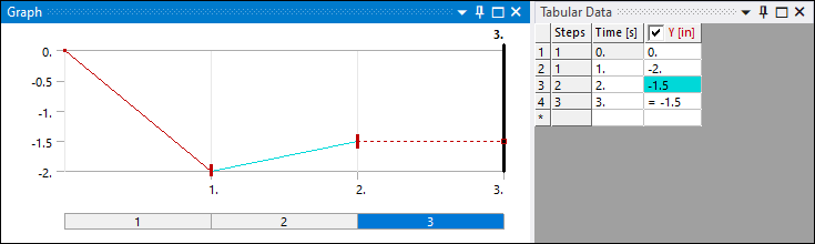
In this example the second step has a displacement value of -1.5. However since the load is deactivated this will not have any effect until the third step. In the third step a displacement of -1.5 will be step applied from the sprung-back location.