


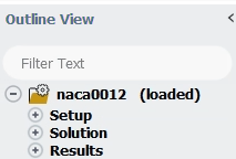
Once a simulation is loaded, a simulation tree appears in the Outline View. The name of the simulation you have loaded appears at the top of the tree along with the text (loaded). Underneath the name of the simulation, the tree is composed of three main branches.
Setup, Solution and Results.
Setup
Defines the type of simulation, the in-flight icing conditions, the physical models and the boundary conditions to use in your simulation.
Solution
Defines the solver settings of your in-flight icing simulation including monitoring, initialization and output files.
Results
Allows post-processing of your in-flight icing results.
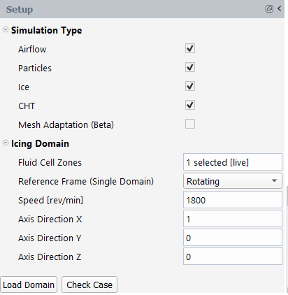
Simulation Type
To start your simulation, you must define its type. Three types are provided when selecting the Setup branch.
Airflow
The airflow solver. Two solvers are supported ( and ).
The particle impingement solver, in this case DROP3D. Vapor transport can also be enabled as part of the Particles solution. An airflow solution is required to conduct this simulation.
Ice
The ice accretion solver, in this case ICE3D. An airflow and particles solution are required to conduct this simulation.
CHT
Conjugate heat transfer (CHT) module that couples Fluent’s intrinsic CHT with the icing solver. A converged dry air CHT, particle and initial ice solution are required to conduct this simulation.
Therefore, five combinations of simulation types are supported:
Stand-alone Airflow simulation
Stand-alone Particles simulation, with an airflow solution already loaded.
Stand-alone Ice simulation, an Airflow and Particles solution already loaded.
An Airflow + Particles simulation. Each simulation is run in sequence.
An Airflow + Particles + Ice simulation. Each simulation is run in sequence. This combination allows the simulation of single and multiple quasi-steady (multi-shot) ice accretion calculations.
Stand-alone CHT simulation, with an Airflow, Particles, and Ice solution already loaded.
Disabling a Simulation Type from the Setup window will hide its relevant settings from the Outline View.
Airflow conditions are used by all four simulation types and Particles conditions are required for Ice.
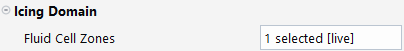
Icing Domain
A Fluent case might contain multiple cell zones (fluid or solid) or domains. By default, Fluent Icing will consider all cell zones as the icing domain. To specify the correct fluid cell zones in the multiple cell zones scenario, enable the checkbox and select the desired ones from the zone list.
For simulations with rotating components like propellers and engine rotors, the Reference Frame should be set to . This will activate the rotational frame formulation for the equations of motion in all solvers, applying a rotation vector defined as revolutions per minute (rpm) along the axis specified in this panel. If there are static walls in the domain (shrouds, splitters, etc.), they will have to be given the opposite rotation speed in their respective boundary condition section.
Once the domain is selected, use the button to properly set the domain.
The list of Boundary Conditions is restricted to the zones enclosing the selected domains
Mesh and nodal solutions used by the Icing solvers will be restricted to the selected domains.
The Icing Domain selection does not affect a Fluent airflow calculation launched from Fluent Icing.
Post-processing of particles and icing solutions using Viewmerical or CFD-Post will only be done on the selected domains.
Note: Solutions obtained on a different subset of domains cannot be loaded.
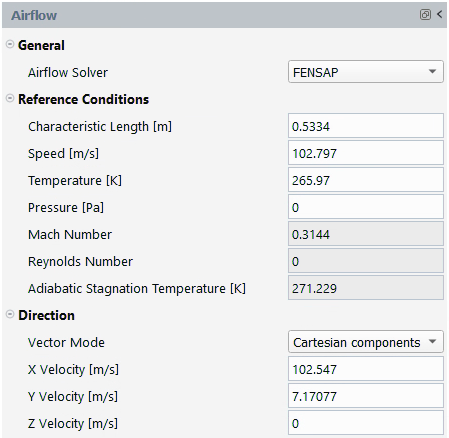
The Airflow window defines the airflow solver, the airflow conditions and the direction of the icing simulation.
General
Choose between and as the Airflow solver. Your choice will appear in the Outline View as an Airflow branch under Setup. Clicking this branch will allow the set-up of the air properties and physical models of either Fluent or FENSAP.
Conditions
These are the reference airflow conditions used by all simulation types. By default, its values are copied from the Reference Conditions of the case file.
The table below connects these variables to FENSAP-ICE or Fluent variables.
| Fluent Icing | FENSAP-ICE | Fluent |
|---|---|---|
| Characteristic Length [m] | Characteristic length | Length |
| Speed [m/s] | Air velocity | Velocity |
| Temperature [K] | Air static temperature | Temperature |
|
Pressure [Pa] (Corresponds to the absolute air static pressure of FENSAP and is the sum of the Operating Pressure and the Reference Pressure in Fluent. | Air static pressure (FENSAP only supports absolute pressure quantities). | Reference Pressure |
| Operating Pressure | Operating Pressure |
Note: When modifying the Pressure [Pa] in Fluent Icing you are modifying the Reference Pressure in Fluent while the Operating Pressure remains equal to the original value from the case file. If you wish to modify the Operating Pressure, you will need to update the other pressure values at the boundaries or in the Initialization section at the same time within the Fluent workspace.
Direction
Two approaches to specify the orientation of the reference airflow are supported.
Cartesian components
The direction is specified by assigning velocity components in X, Y and Z.
Angle of attack
The direction of the flow is specified via two angles, AoA [deg.] and Yaw [deg.] and its velocity magnitude by Velocity magnitude [m/s]. The planes on which these two angles are defined are obtained by selecting the coordinate axis of lift (Lift Direction) and drag (Drag Direction) for a zero degree AoA. The AoA is defined on the plane consisting of the Drag Direction as the primary axis and the Lift Direction as the secondary axis, while the Yaw angle is defined on the plane consisting of the Drag Direction as the primary axis and the result of the cross product of Drag Direction x Lift Direction as the secondary axis.
For instance, if the Drag Direction is set to X+ and the Lift Direction is set to Y+, the flow direction will be defined by the X+ axis if you set the AoA [deg.] and Yaw [deg.] to 0 degree. If the AoA [deg.] is set to
90degrees and the Yaw [deg.] is set to0degree, the flow will be entirely in the Y+ direction. If the AoA [deg.] is set to0degree and the Yaw [deg.] is set to90degrees, the flow will be entirely in the Z+ direction.
Fluent Airflow Solver
If Fluent has been selected as the Airflow solver in the Airflow window, the Fluent window appears if you click Setup → Airflow → Fluent. In this window, you can specify the material properties of air and the most common physical models of air used for icing simulations.
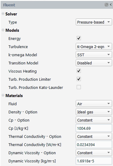
For more information regarding recommendations on how to set-up air properties and physical models in Fluent, consult Recommended Settings.
Materials
Set the same air properties as the ones coming from the loaded case file (Fluid set to Case settings) or set new air properties (Fluid set to Air).
The parameters shown below Fluid are the Fluent parameters and they only appear if Fluid is set to . For icing simulations, you should set Density to and the remaining properties using the Recommended Settings. Alternatively, this could be done by right-clicking Fluent in the Outline View and then by selecting .
Models
The parameters shown in Models are the Fluent parameters under Setup → Models. Only the physical models recommended in Recommendations to Set up a Fluent Calculation are provided. Follow Recommended Settings to select the appropriate models for icing calculations.
The Other flag is displayed next to Turbulence when the case file contains a viscous model that is different than the ones supported by Fluent Icing (k-Omega 2-eqn and Transition SST 4-eqn).
Although viscous heating and energy appear as options here to be compatible with standard Fluent setup, they must be enabled for icing simulations otherwise heat transfer coefficients used in the ice accretion model will not be calculated correctly.
Solver
Select which Fluent solver type to use: or . Refer to Overview of Using the Solver in the Fluent User's Guide for more information about these solver types.
Commands
Access the following commands by right-clicking Fluent, located in Setup → Airflow → Fluent.
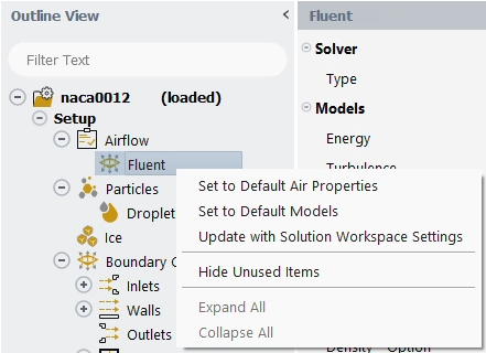
Set to Default Air Properties
Changes the current material to Air and will set the air material properties to the Recommended settings for icing simulations, see Recommended Settings.
Set to Default Models
Enable the Recommended settings for models. See Recommended Settings.
Update with Solution Workspace Settings
Use this option to synchronize your Solution workspace or background solver session changes with Fluent Icing.
Note: Changes made to Fluent Icing are automatically synchronized with simulation workspace.
Recommended Settings
When performing icing simulations using Fluent as the airflow solver, the following Material settings for Air are recommended. These can be automatically set by right-clicking the Fluent node under Airflow and choosing .
Set the Density - Option to ideal-gas
Set Cp [J/kg-K] to
1004.688. This value is equal to γ/(γ-1)*R, where γ = 1.4 and the gas constant R = 287.05376 J/kg-K.Set the Thermal Conductivity - Option to Constant and set Thermal Conductivity [W/m-K] to an appropriate value for the condition. To compute its value, refer to the thermal conductivity equation below.
Set the Dynamic Viscosity - Option to Constant, and set Dynamic Viscosity [kg/m-s] to an appropriate value for the condition. To compute its value, refer to the viscosity equation below.
Use the following equations to compute the thermal conductivity and dynamic viscosity, respectively.
Furthermore, the following Model settings are recommended.
Energy must be enabled for icing simulations.
The Turbulence model with is recommended for icing simulations.
and must be enabled for icing simulations.

FENSAP Airflow Solver
If is selected as the airflow solver in the Airflow window, the following FENSAP window appears when selecting → → .
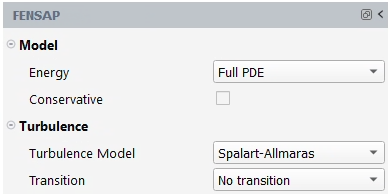
In this new window, you can specify the most common physical models of air used in icing simulations.
The most common airflow properties of FENSAP for icing simulations are the ideal gas properties with constant thermal conductivity and dynamic viscosity as specified in the Recommended Settings.
Model
In Fluent Icing, the momentum equations are always set to Navier-Stokes and three options are available for Energy.
Full PDE, Constant enthalpy and Energy only. Full PDE is the most common option for icing applications. By default, FENSAP solves the energy equation in non-conservative form which results in robust convergence especially when the momentum and energy systems are uncoupled. To solve the energy equation in conservative form, enable Conservative. The conservative formulation improves heat flux accuracy for transonic speeds and above, but may require a lower CFL number to converge.
For more information regarding these settings, consult The Energy Equation.
Turbulence
All turbulence and transition models of FENSAP are supported in Fluent Icing. The default settings (SA with no transition) are the most common for ice accretion simulations. For more information regarding these models, consult section Turbulent Flows and Transition to Turbulence.
Note: Default numerical convergence settings are applied to all turbulence models of FENSAP.
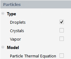
The Particles window defines the type of particles to simulate and the activation of the particle thermal equation that models the temperature and phase change of particles. The particle thermal equation would be important when solving flows with hot exhausts, and internal flows in turbomachinery components.
Note: Air/particle momentum coupling is modeled 1-way where air is not affected by particles. In general, icing cloud particle volume fraction is in the order of 1e-6, making this a dilute particle flow problem. Therefore, in in-flight icing simulations particle flow computations are done segregated from the air flow. This simplifies the modeling process and makes it more cost efficient.
The thermal coupling between air and particles can be significant, and requires 2-way coupling of the energy equations plus vapor transport. In FENSAP-ICE, this is done by solving in mode with the energy-only mode for airflow. This option is currently not available in Fluent Icing.
Type
Three particle types are supported:
Droplets
Supercooled water droplets that are still in liquid form at lower ambient temperatures. They typically accrete ice on external aircraft surfaces.
Crystals
Ice crystals are solid ice particles of various shapes and sizes that are suspended in air. They bounce off cold external aircraft surfaces but typically accrete on warm internal surfaces (engine components) where they can melt and stick.
Vapor
Water vapor pressure determines the evaporation rate on icing surfaces, which is a strong thermal flux that leads to ice formation. Water vapor also acts as a mode of energy transport where warm droplets can shed heat in the form of evaporated mass which can be recovered later in the form of condensation onto particles. For external icing problems inclusion of vapor transport in the modeling process makes very little difference in the results.
Vapor transport model features a simplified nucleation model where any vapor mass greater than local saturation point is considered to have nucleated. This limits the maximum observable relative humidity to 100% in the solution domain, and clips the maximum vapor pressure to local saturation pressure. In FENSAP-ICE, thermal coupling with the airflow solver transfers the released latent heat of evaporation to the air. Since Air+Droplets mode is currently not available in Fluent Icing, this energy source is ignored.
These particle types can be selected concurrently and therefore can all be simulated simultaneously within the same Particle simulation.
Enabling a particle Type from the Particles window will create its corresponding branch under Particles as well as any other relevant setting related to this particle type in Boundary Conditions and Solution.
Model
By default, continuity and momentum equations of droplets and crystals, and continuity equations of vapor are always solved when these particles are selected in Type. These are the typical equations needed to study external in-flight icing physics. For more information regarding these equations, consult The Particle Transport System and Supercooled Large Droplets (SLD).
To activate the energy transfer between particles as well as their respective phase change, the Particle Thermal Equation must be enabled. You should enable this option when studying internal in-flight icing physics, for example, inside engines.
Reinjection
When either Droplets or Crystals particle types are selected, external reinjection can be solved. The primary solution will be used to evaluate the mass of particles which splashes (droplets) or bounces (crystals) at the walls.
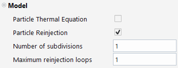
Number of Subdivisions
When is enabled, the wall conditions are split into a Number of subdivisions. A new independent particle run will be solved for each of these subdivisions to account for the crossing of reinjected particles trajectories.
Maximum Reinjection Loops
When is enabled, reinjected particles can hit the wall several times before exiting the domain. The particle wall interaction will be solved until no reinjected particle hits the wall or the specified Maximum reinjection loops is reached.
Droplets
If Droplets is selected as a particle Type in the Particles window, the following Droplets window appears when you click Setup → Particles → Droplets.
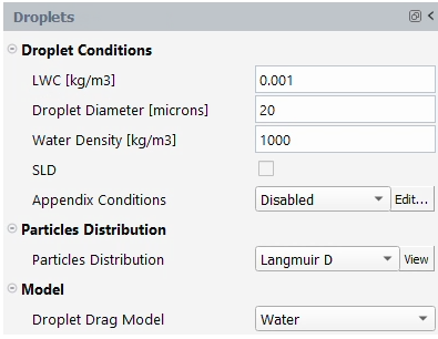
In this window, you can specify the ambient/reference conditions of water droplets, the type and size distribution, and the drag model.
Droplet Conditions
The main physical parameters describing the droplets are:
LWC [kg/m3]
The Liquid Water Content (LWC) is the concentration of water droplets in the air.
Droplet Diameter [microns]
Spherical droplets are assumed to be of a single, uniform size, usually equal to the median volume diameter (MVD) of the sample size distribution. In Particles, the droplet diameter is the MVD.
Water Density [kg/m3]
This is the density of the water droplets. By default, its value is set to 1,000 kg/m3.
SLD
Supercooled Large Droplets (SLD) options allow the set-up of extra physical models when water droplets exceed a MVD of ~40 microns.
Note: When particle reinjection is enabled, SLD is automatically selected.
Appendix Conditions
Appendix conditions are recognized droplet cloud environments that linked ambient conditions to average droplet sizes and concentrations. Select the appropriate Appendix Conditions drop-down, then use the button located to the right of the Appendix Conditions menu. This will automatically set LWC [kg/m3] and Droplet Diameter [microns] to use in your simulation.
Note: The altitude in the Appendix Conditions panel is computed from the absolute pressure defined under Setup → Airflow → Conditions. If the altitude is modified, a new Pressure [Pa] value is automatically computed and imposed under Setup → Airflow → Conditions. However, this is not the case for the boundary conditions. It is therefore recommended to manually update Pressure [Pa] at the inlet and outlets of your farfield domain by first setting the boundary under Setup → Airflow → Conditions to . You can then either copy the new reference pressure inside Pressure [Pa] at the boundary, or by click the button located at the bottom of your boundary condition panel.
The following droplet appendices are supported:
Appendix C
In general, valid for droplet sizes below 40 microns.
Appendix O (SLD)
In general, valid for droplet sizes that exceed 40 microns. To use , SLD must be enabled.
Inside each Appendix panel, ambient conditions such as air temperature and altitude are taken from the submenu inside the Airflow panel. In this case, altitude and absolute pressure follow the U.S. Standard Atmosphere (1976).
Note: Only one Appendix can be activated at a time. For more information regarding these appendices, consult Appendix C and Appendix O - Supercooled Large Droplets.
Only built-in droplet size distributions are currently supported by Fluent Icing. These distributions can be selected in the Droplet Distribution pull-down menu.
Monodispersed
Indicates that a calculation is performed using a single diameter. This diameter is specified in the Droplet diameter box and corresponds to the MVD.
Langmuir B to E
If one of these is selected, water droplets are simulated by computing the droplet concentration and speed for each individual diameter of the discrete distribution, which are subsequently automatically weight-averaged at the end of the simulation. Fluent Icing always uses 7 droplet diameters to represent a Langmuir B to E distribution. The various Langmuir diameter distributions and their corresponding weights are pre-defined in FENSAP-ICE. To learn more about these distributions and their respective weights, consult Droplets Reference Conditions. The distribution can be viewed by using the button on the right side of the distribution menu.
An arbitrary droplet diameter distribution can be set by using the button on the right side of the distribution menu.
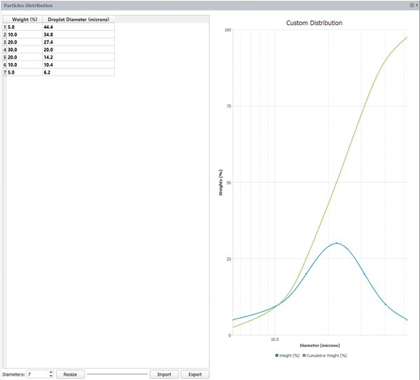
The Particles Distribution panel allows you to edit the weight/diameter distribution table.
: The button is for read-only distributions ( or ) and permit to toggle the distribution in Edit mode, the distribution setting is then set to Custom.
: Change the number of rows in the particles distribution table.
/ : Reads or writes a .csv file with the following format, for example for the equivalent distribution of a with a MVD of 20 microns:
Weight,Diameter
0.05,44.4
0.1,34.8
0.2,27.4
0.3,20
0.2,14.2
0.1,10.4
0.05,6.2
The Particles Distribution must be defined as following:
Droplet Diameter (microns): Diameters ordered in increasing or decreasing order.
Weight (%): Sum of weights adding up to 100%.
If an individual value or a whole column is invalid, it will be highlighted in yellow.
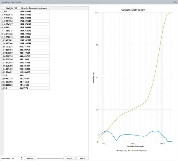
If the Appendix Conditions is set to , the Droplet Distribution can be either or . See Appendix O - Supercooled Large Droplets in the Ansys FENSAP-ICE User Manual for more details.
The selected distribution can be viewed using the button, right side of the distribution menu. The Appendix O (SLD) distribution depends on the environment (freezing drizzle, freezing rain) or diameter range (larger or lower than 40 microns) selected in its Particles Distribution panel.
Model
In this submenu, different water droplet physical models can be enabled to better represent their behavior for higher Weber numbers. Some of these models are only available when the SLD option is enabled under Droplet Conditions.
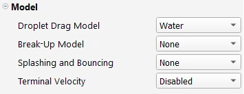
General Models
Droplet Drag Model
These models correspond to drag correlations. Four choices are available (Water, Water -Stokes law, Water – extended Reynolds, Snowflakes). The default drag model is set to Water, which is the drag model used in almost all our water droplet validation cases. For more information regarding these models, consult Particle Drag Correlations.
SLD-Only Models
Break-up Model
Models the process by which a large droplet is broken up into smaller droplets due to aerodynamic forces. To enable this model, select Pilch & Erdman, the only break model supported in FENSAP-ICE. If selected, an extra governing equation is solved for droplet diameter. For more information regarding this model, consult Droplet Break-Up. This option is automatically selected when external reinjection is enabled.
Splashing and Bouncing
Only the By post-processing with three splashing models (Mundo, Honsek and Wright) are supported in Fluent Icing. These are the most validated models used in SLD splashing & bouncing simulations, with a preference for Mundo, default Splashing Model setting. They modify the droplet collection efficiency on the surface by predicting if water droplets bounce or splash. Droplets that bounce or splash are not re-introduced into the computational domain. For more information regarding these models, consult Splashing and Bouncing by Post-Processing, Mundo Model, Honsek-Habashi Model and Wright-Potapczuk Model in the Ansys FENSAP-ICE User Manual. If reinjection is enabled, the selected splashing model is used to evaluate the mass of reinjected droplets.
Terminal Velocity
This option enables supercooled large droplets to fall without exceeding their terminal velocity. This option will alter the transport of droplets and therefore its impingement. The direction and the magnitude of the gravity vector must be specified in the case file. For more information regarding this model, consult Terminal Velocity. Pay attention to the gravity direction specification with respect to the mesh coordinate system. An aircraft at level flight usually has a small positive angle of attack which has to be factored into the gravity direction. An aircraft during climb has a positive vertical speed component in addition to a significant angle of attack with respect to that flight direction, both of which should be considered when specifying the gravity vector.
Crystals
If Crystals has been selected as a particle Type in the Particles window, the following Crystals window appears when you click Setup → Particles → Crystals.
In this window, you can specify the ambient/reference conditions of crystals.
Note: Only one drag model of crystals has been implemented and it follows the oblate spheroidal drag correlation formulated by Pitter. For more information regarding this model, consult Ice Crystal Drag Correlations.
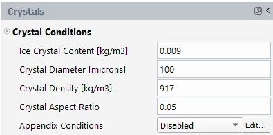
Crystal Conditions
The main physical parameters describing the ice crystals are:
Ice Crystal Content [kg/m3]
The Ice Crystal Content (ICC) is the concentration of crystals in the air.
Crystal Diameter [microns]
Ice crystals are assumed to be of a single, uniform size. In this case, the crystal diameter corresponds of the semi-major axis length of a thin oblate spheroid.
Crystal Density [kg/m3]
This is the density of the ice that forms the ice crystal. By default, its value is set to 917 kg/m3.
Crystal Aspect Ratio
This is the aspect ratio (E=b/a) of an oblate spheroid, where b is the semi-major axis length and a is the semi-minor axis length.
Note: Icing wind tunnel experiments with glaciated droplets usually lead to aspect ratios around 1. Increasing the aspect ratio increases the drag of the crystals and make them follow the air more closely, decreasing their collection efficiency.
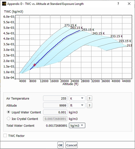
Appendix Conditions
Only one recognized cloud environment type condition for crystals is supported in Fluent Icing, it is . If this option is enabled, use the button located at the bottom of the property panel. This will automatically set the ICC and the LWC to use in your simulation since Appendix D defines the Total Water Content (TWC).
Inside the Appendix D panel, ambient conditions such as air temperature and altitude are taken from the Conditions submenu inside the Airflow panel. In this case, altitude and absolute pressure follow the U.S. Standard Atmosphere (1976).
Note: Only one Appendix can be activated at a time. For more information regarding Appendix D, consult Appendix D - Ice Crystals.
Crystal Distributions
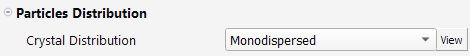
If are the only particles type enabled ( are not enabled), the Particles Distribution panel is available and allows you to configure a diameter distribution.
Indicates that a calculation is performed using a single diameter. This diameter is specified in the Crystal Diameter (microns) box and corresponds to the MVD.
An arbitrary crystal diameter distribution can be set by using the button on the right side of the distribution menu. Similar to under Particles Distribution.
A custom crystal distribution allows you to define both Crystal Diameter (microns), and Crystal AR (Aspect Ratio).
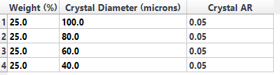
The .csv file format for / contains that extra aspect ratio column, such as:
Weight,Diameter,Aspect Ratio
25,100,5.0e-02
25,80,5.0e-02
25,60,5.0e-02
25,40,5.0e-02
Vapor
If Vapor has been selected as a particle Type in the Particles window, the following Vapor window appears when you click Setup → Particles → Vapor. In this window, you can specify the ambient/reference conditions of vapor.
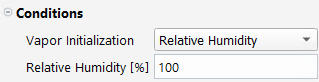
Conditions
The main physical parameters describing vapor are:
Relative Humidity [%]
This option is enabled if selected under Vapor Initialization. This option corresponds to the ambient relative humidity and ranges from 0 to 100 %. It is defined as the ratio of partial vapor pressure to the saturation vapor pressure.
Vapor Concentration [kg/m3]
This option is enabled if selected under Vapor Initialization. This option corresponds to the ambient vapor concentration.
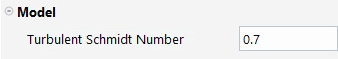
Turbulent Schmidt Number
If are enabled through → → Icing, Turbulent Schmidt Number can also be specified. The default value is 0.7.
The Ice window defines the icing conditions and the icing physical models to use during the ice accretion simulation.
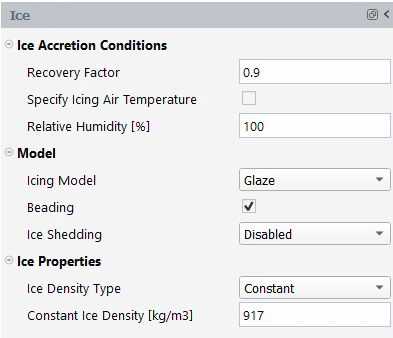
Ice Accretion Conditions
The main physical parameters describing the ice accretion process are:
Recovery Factor
The recovery factor is used to introduce the effect of the energy losses due to friction when computing the adiabatic/recovery temperature at the wall. This is a factor that is used to compute the convective heat transfer coefficients in FENSAP-ICE for ambient/reference or icing temperatures. Its default value is 0.9 (~Pr1/3) is observed on flat plate experiments. This is the value used in FENSAP-ICE ice shape validation cases. On wing and airfoil stagnation points, the value of the recovery factor is closer to 1. Using 1 instead of 0.9 will increase the amount of water film runback.
Specify Icing Air Temperature
The Icing Air Temperature [K] is the static temperature at which ice accretion is computed. This temperature can therefore be different than the ambient air temperature specified in the Airflow window or inside your inlet boundary conditions. If the energy equation of particles is enabled, the icing air temperature must be the ambient air temperature specified in the Airflow window. This option cannot be used in multi-shot computations. It is automatically disabled for multi-shot ice accretion.
Relative Humidity [%]
This is the relative humidity expressed in percentage value. For atmospheric clouds, this value should be set to 100%. If is enabled in Particles, this parameter is disabled, and ignored. The vapor pressure field computed in the vapor transport model is used on walls when calculating the rate of water film evaporation.
For more information regarding these parameters, consult Icing Conditions.
Model
The main physical models describing the ice accretion process are:
Icing Model
The icing models solve the surface water film continuity and energy equations using an explicit unsteady 3D finite volume scheme (see Governing Equations) in different forms.
Glaze
Glaze icing model is meant for glaze and mixed type ice shapes including water runback and evaporation. This is the most comprehensive model that can operate above and below freezing temperatures and produce rime ice with no water film, glaze ice with water film at 0° C, and all water above freezing temperature that can form in anti-icing and de-icing scenarios.
Water film
This model engages the pure water film mode where the energy equation is used to calculate water temperature instead of ice accretion rate. It is meant for water film runback simulations at above freezing conditions.
Rime
In rime mode, no runback is assumed, and the continuity equation simply dictates the rate of icing. The energy equation is used to compute the below freezing ice temperature.
Beading
When enabled, the beading model calculates variable surface roughness evolution on iced walls. The resultant roughness is expressed as equivalent sand-grain roughness. During a multi-shot simulation this sand-grain roughness affects the convective heat fluxes and therefore the local cooling effects over iced surfaces. Most importantly, it eliminates the guess work of choosing a constant wall roughness which would be applied to the entire wall uniformly. You should activate this model to obtain accurate multi-shot results.
Heat Flux
This option is only visible if the Airflow Solver is set to , and are enabled through → → Icing. This option allows the selection of two types of convective heat flux produced by FENSAP to conduct an ice accretion simulation.
Convective heat fluxes computed using temperature gradients on the walls. This method is 2nd order accurate and is the default option when is disabled.
Convective heat fluxes computed based on Gresho’s Consistent Galerkin formulation. Gresho fluxes tend to exhibit oscillations when the surface grid is uneven or coarse and therefore it is less robust than .
Ice Shedding
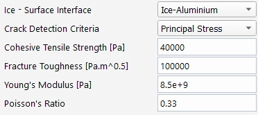
This option enables ice stress and crack propagation analysis in single-shot icing simulations. Currently, it is only meant for rotating components where loads on the ice are primarily due to the centrifugal forces. With this feature, you can simulate the natural ice shedding phenomenon on aircraft components like propellers and engine fans. For more information on the model, see Ice Shedding on Rotating Components.
When enabled, additional ice properties will be listed below that are required for the ice stress and crack propagation analysis.
Crystals
appears in the Ice window if Crystals has been selected in the Particles window. enables the contribution of crystals to the icing calculation, otherwise, Ice assumes that all crystals bounce off the surface, . Two bouncing models are available.
NTI Bouncing Model
This model determines the amount of crystals that stick based on local surface conditions, such as impact velocity, crystal size and film height. The model also includes an optional feature to account for crystal Erosion effects on ice accreting surfaces.
NRC Bouncing Model
This model calculates the sticking faction based on the LWC to TWC ratio hitting the surface.
Ice Properties
Ice Density Type
There are five models to specify the ice density in Fluent Icing Constant, Macklin, Jones Glaze, Jones Rime and Impact Ice Density: By default, a constant value of 917 kg/m3 is set. The other density types are correlations that uses the local ice surface temperature and other icing conditions. For more information regarding these ice density correlations, consult Ice Density. The other density types are correlations that uses the local ice surface temperature and other icing conditions. For more information regarding these ice density correlations, consult Ice Density.
Impact Ice Density Model
The Impact Ice Density model is created by Ansys especially for swept wing icing simulations, inspired by the void density model in NASA’s LEWICE3D. It is meant to be used as part of multishot icing with remeshing workflow, to help generate realistic ice shapes with feathers and scallops. The studies for the AIAA Ice Prediction Workshops showed that this density model is essential in capturing accurate scallop formations that produce valid Maximum Combined Cross Sections (MCCS) both for glaze and rime conditions. It uses local droplet impact angle and freezing fraction to vary the density from 917 kg/m3 to 200 kg/m3. Perpendicular impact and low freezing fraction increase the density of ice which is closer to glaze ice, and the opposite reduces the density resembling feathery ice observed near the impingement limits of aircraft surfaces.
The model is controlled by three parameters: minimum rime ice density, maximum rime ice density, and blending coefficient:
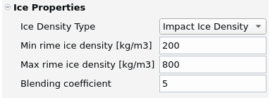
For glaze ice conditions where the freezing fraction is closer to 0, the ice density will be closer to 917 kg/m3. In rime ice conditions, the ice density will be set between min and max rime ice density values entered in this panel. The maximum rime ice density value is used when the impact angle of droplets is 90O (perpendicular) to the surface. The minimum ice density value is set for impact angle = 0O (tangent), which is a theoretical value that droplets will get close to at impingement limits. The change from maximum to minimum rime ice density based on the impact angle value is done with a non-linear blending function, which is controlled by the blending coefficient. The range for this coefficient is 2 – 10. Higher blending coefficient values keep the ice density high for a wider range of impact angles. Currently the recommended value is 5, which is determined based on the swept wing ice accretion results from 1st and 2nd AIAA Ice Prediction Workshops. More details are provided in Ansys FENSAP-ICE User Manual for this model.
Partial differential equations are solved for each Fluent Icing module. Therefore, each module requires a set of suitable boundary conditions. The options shown in each boundary condition type reflect the simulation type, conditions and physical models selected/enabled in Airflow, Particles and Ice.
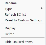
Note: Fluent Icing offers the option to modify boundary condition types to those supported by Fluent Icing. Only a couple of boundary condition types are currently supported by Fluent Icing. Boundary condition types can also be modified from the background solver session that is connected to Fluent Icing (by using ). These changes can be viewed in Fluent Icing by right-clicking any boundary condition type inside the Outline View and selecting Refresh BC List. Only supported boundary condition types are shown in Fluent Icing.
The right-click menu for each boundary offers options to rename, refresh, change type, and reset to custom settings if needed.
Only a couple of Fluent boundary condition types are currently supported by Fluent Icing.
Inlets
Pressure-far-field
Velocity Inlet
Mass-flow Inlet
Pressure Inlet
Walls
Outlets
Pressure Outlet
Symmetry
Periodic
In the next sections, a brief description of the content of Inlets, Outlets and Walls is provided. Symmetry and periodic types do not require a specific set-up for icing applications and therefore are not describe here.
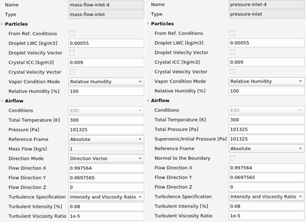
Ice accretion simulations require inlet airflow and particles boundary conditions. Four types of Fluent boundary conditions are supported to simulate the Airflow module of Fluent Icing. Since the Particles module only supports Dirichlet boundary conditions, particle concentration and velocity conditions are specified on all Fluent boundary types.
The following figures show each Inlet boundary type supported by Fluent Icing when all particles type are enabled.
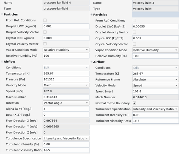
Airflow
To simplify set-up of the Airflow solver, it is possible to automatically define the boundary conditions for all the Inlet types by selecting one of the two options under Conditions.
Case settings
With this option, inlet boundary conditions are automatically taken from your case file. Therefore, this is only available if a case file has been set up beforehand with the Fluent Solution workspace.
Edit
With this option, you can define boundary conditions that are different than those contained in the original case file or in the Airflow settings.
The following tables map the Fluent Icing airflow boundary conditions to Fluent and FENSAP airflow boundary conditions when Edit is selected.
Table 2.1: Pressure Far-Field, Mapping of Airflow Fluent Icing Boundary Condition into Fluent & FENSAP Boundary Conditions
| Fluent Icing | Fluent | FENSAP | ||
|---|---|---|---|---|
| Type: Pressure-far-field | Type: Pressure-far-field | Type: Supersonic or Far-field | ||
| Temperature [K] | Temperature (k) | Temperature | ||
| Pressure [Pa] (Absolute) | Gauge Pressure (pascal) | Pressure | ||
| Velocity mode | ||||
| Speed [m/s] | --------- | --------- | ||
| Mach number | Mach number | --------- | ||
| Direction mode | --------- | |||
| Vector Components | --------- | |||
| Flow direction X | X-Component of Flow Direction | Velocity X | ||
| Flow direction Y | Y-Component of Flow Direction | Velocity Y | ||
| Flow direction Z | Z-Component of Flow Direction | Velocity Z | ||
| Vector Angle | ||||
| Alpha (X-Y) [deg] | --------- | --------- | ||
| Beta (X-Z) [deg] | --------- | --------- | ||
Table 2.2: Velocity Inlet, Mapping of Airflow Fluent Icing Boundary Condition into Fluent & FENSAP Boundary Conditions
| Fluent Icing | Fluent | FENSAP | |||
|---|---|---|---|---|---|
| Type: Velocity Inlet | Type: Velocity Inlet | Type: Subsonic | |||
| Temperature [K] | Temperature (k) | Temperature | |||
| Pressure [Pa] (Absolute) | Supersonic / Initial Gauge Pressure (pascal) | --------- | |||
| Velocity Mode | |||||
| Speed [m/s] | Velocity Magnitude (m/s) | --------- | |||
| Mach number | --------- | --------- | |||
| Normal to the boundary | Magnitude, Normal to Boundary | --------- | |||
| Direction | |||||
| Vector Components | |||||
| Flow direction X | X-Component of Flow Direction | Velocity X | |||
| Flow direction Y | Y-Component of Flow Direction | Velocity Y | |||
| Flow direction Z | Z-Component of Flow Direction | Velocity Z | |||
| Vector Angle | |||||
| Alpha (X-Y) [deg] | --------- | --------- | |||
| Beta (X-Z) [deg] | --------- | --------- | |||
Table 2.3: Mass Flow Inlet, Mapping of Airflow Fluent Icing Boundary Condition into Fluent & FENSAP Boundary Conditions
| Fluent Icing | Fluent | FENSAP | ||
|---|---|---|---|---|
| Type: Mass Flow Inlet | Type: Mass Flow Inlet | Type: Mass Flow | ||
| Temperature [K] | Total Temperature (k) | Static Temperature | ||
| Pressure [Pa] (Absolute) | Supersonic / Initial Gauge Pressure (pascal) | -------- | ||
| Direction mode | --------- | -------- | ||
| Direction Vector | ||||
| Mass Flow [kg/s] | Mass Flow Rate (kg/s) | Mass Flow | ||
| Flow direction X | X-Component of Flow Direction | Alpha & Beta | ||
| Flow direction Y | Y-Component of Flow Direction | |||
| Flow direction Z | Z-Component of Flow Direction | |||
| Normal to Boundary | ||||
| Mass Flow [kg/s] | Mass Flow Rate (kg/s) | -------- | ||
Table 2.4: Pressure Inlet, Mapping of Airflow Fluent Icing Boundary Condition Into Fluent Boundary Conditions
| Fluent Icing | Fluent | |
|---|---|---|
| Type: Pressure Inlet | Type: Pressure Inlet | |
| Temperature [K] | Total Temperature (k) | |
| Total Pressure [Pa] (Absolute) | Supersonic / Initial Gauge Pressure (pascal) | |
| Normal to the boundary | Normal to Boundary | |
| Flow direction X | X-Component of Flow Direction | |
| Flow direction Y | Y-Component of Flow Direction | |
| Flow direction Z | Z-Component of Flow Direction | |
Note: Reference Frame allows the inlets to be defined relative to a cell zone motion or in absolute reference frame. This does not apply to fixed cell zones. However, if a rotating domain is defined, the inlet properties (for example, Flow Direction) can be defined relative to the domain motion.
Velocity Mode allows the use of Speed [m/s] or Mach Number as a boundary condition when the Inlet is a or a .
Normal to the Boundary defines the flow direction using the normal vectors of the boundary surface. If selected, the Direction options do not appear. This option only appears when the inlet is a .
Direction allows the specification of three types of flow direction at the inlet of a or .
Vector Components
If selected, the orientation of the inlet flow is defined by the following unit vector components, Flow Direction X, Flow Direction Y and Flow Direction Z.
Vector Angle
If selected, the orientation of the inlet flow is defined by the following angles, Alpha (X-Y) [deg] and Beta (X-Z) [deg].
Case settings
If selected, the orientation of the inlet flow is defined by the orientation used in the case file.
Direction Mode allows the definition of two types of flow direction at the inlet of a Mass Flow Inlet.
Direction Vector
If selected, the orientation of the inlet flow is defined by the following normalized flow components, Flow Direction X, Flow Direction Y and Flow Direction Z.
Normal to Boundary
If selected, the orientation of the inlet flow is defined by the normal vectors of the boundary surface.
Italic Fluent and FENSAP boundary conditions shown in the mapping tables highlight conditions that do not have a perfect counterpart in Fluent Icing.
Fluent
X/Y/Z-Component of Flow Direction
The Flow orientation in Fluent can be defined by a non-unitary vector. However, when using Fluent Icing, this orientation must be provided as a normalized vector.
Total Temperature [K]
When using Fluent as the Airflow solver in Fluent Icing, write the total temperature of a mass flow or pressure inlet boundary condition type inside Temperature.
FENSAP
Alpha and Beta angles
These angles are not supported by Fluent Icing. In FENSAP, Alpha is the angle in the X-Y plane and Beta is the angle in the X-Z plane. Transform these angles to normalized vector components and impose them as boundary conditions inside Direction Mode → Direction Vector.
Currently, the Fluent Icing user interface only supports turbulence boundary conditions when using Fluent as the airflow solver.
There are two options available in the current implementation: and . When loading a case file, Fluent Icing will automatically set the Turbulence Specification method to and use the constant values associated with the turbulent intensity and viscosity ratio if they are specified in the case file. Only these turbulence models are currently supported during the import: , , and . For , only the intermittency parameter constant value is imported.
If any of the above-mentioned conditions are not satisfied, Fluent Icing will set the Turbulence Specification method to . The turbulence settings in the case file will be used. You can verify them from the Solution workspace. If you change to within Fluent Icing, the turbulence settings that appear in the Fluent Icing properties panel of will be applied to the Solution workspace.
Note: Only constant values can be set from the Boundary Conditions properties panel in Fluent Icing.
If is selected as the Airflow solver, it is not possible to specify turbulence parameters at the boundary condition; default turbulence boundary conditions are imposed.
SA
Eddy/laminar viscosity ratio of 1e-5
kw-SST
Eddy/laminar viscosity ratio of 1 and Turbulence intensity of 0.01.
To change these default values, use the text commands, Fluent Journal Commands, in the Fluent Console window. For instance, to change the Eddy/laminar viscosity ratio to 1e-3 and the turbulence intensity to 1e-4, type the following commands:
/icing/settings/set
                                                flow/turb_eddy_lam_ratio 1e-3
/icing/settings/set flow/turb_intensity 1e-4
A zero value to these settings will revert them to their default value. Such text commands can also be sent from Fluent Icing by using the
Send Commandaction, in the contextual menu of the case file.
Note: To learn more about these Fluent Inlet boundary conditions, consult Pressure Far-Field Boundary Conditions, Velocity Inlet Boundary Conditions, Mass-Flow Inlet Boundary Conditions and Pressure Inlet Boundary Conditions under Boundary Conditions in the Fluent User's Guide. To learn more about FENSAP Inlet boundary conditions supported in Fluent Icing, consult Inlets and Far-fields – 1000-BCs.
Particles
To simplify set up of the Particles solver, it is possible to automatically define the boundary conditions at the Inlet by checking . In this case, the Particles window settings are applied as boundary conditions and it is assumed that particles and airflow share the same inlet velocity.
The following lists the boundary conditions of all types of Particles when the option is unchecked.
Droplet Boundary Conditions
Droplet boundary conditions are available if Droplets has been selected in Setup → Particles
Droplet LWC [kg/m3]
Set the water droplet concentration at the Inlet.
Droplet Diameter
Set the MVD of the spherical particle that represents a cloud of water droplets at the Inlet. This option is available when the Break-up model has been activated inside Setup → Particles → Droplets.
Droplet Temperature [K]
Set the temperature of the cloud of water droplets at the inlet. This option is available when the Particle Thermal Equation is enabled in Setup → Particles.
Droplet Velocity Vector
When enabled, this option allows the specification of an inlet droplet velocity that is different than the airflow velocity at the inlet. In this case, set the velocity components (Droplet X Velocity [m/s], Droplet Y Velocity [m/s], Droplet Z Velocity [m/s]) of the water droplet cloud.
Crystal Boundary Conditions
Crystal boundary conditions are available if Crystals has been selected in Setup → Particles.
Crystal ICC [kg/m3]
Set the ice crystal concentration at the Inlet.
Crystal Temperature [K]
Set the temperature of the cloud of ice crystals at the inlet. This option is available when the Particle thermal equation is enabled in Setup → Particles.
Crystal Melt Fraction
Set the crystal melt fraction at the inlet if the crystal temperature is equal to the freezing temperature (273.15 K). The crystal melt fraction is automatically set to 0 or 1 if the crystal temperature is lower or higher than 273.15K respectively. This option is available when the is enabled in Setup → Particles.
Crystal Velocity Vector
When enabled, this option allows the specification of an inlet ice crystal velocity that is different than the airflow velocity at the inlet. In this case, set the velocity components (Crystal X Velocity [m/s], Crystal Y Velocity [m/s], Crystal Z Velocity [m/s]) of the ice crystal cloud.
Vapor Boundary Conditions
Vapor boundary conditions are available if Vapor has been selected in Setup → Particles.
Vapor Condition Mode
Set the type of vapor boundary condition to impose at the inlet.
Relative Humidity [%]
Set the relative humidity at the inlet. This value is defined as the ratio of partial vapor pressure to the saturation vapor pressure.
Vapor Concentration [kg/m3]
Set the vapor concentration at the inlet.
Note: In the case of Inlet boundaries that share inlet and outlet cells, the Particles solver will identify the cells that are inlets based on the velocity components of droplets and crystals that have been specified under Particles.
Built-in Inlet type commands are available by right-clicking the inlet type icon in the Outline View or by pressing on the buttons located at the bottom of the Inlet properties window. Two commands are currently supported.
Copies the Airflow settings into the Airflow submenu of the Inlet window when Edit is selected in Conditions.
Display
Displays the surface mesh of the Inlet type selected in the Graphics window.
Ice accretion simulations require appropriate airflow, vapor and icing wall boundary conditions. The following figure shows each Wall boundary type supported by Fluent Icing.
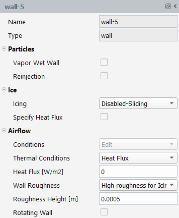
Airflow
In the current version of Fluent Icing, all walls with no slip condition unless otherwise specified in the original case file. The no slip condition is a requirement for computing heat transfer coefficients on walls that are to be enabled for ice accretion.
The following table maps the Fluent Icing airflow wall boundary conditions to Fluent wall boundary conditions.
Mapping of Airflow Fluent Icing Wall Boundary Conditions into Fluent & FENSAP Boundary Conditions.
| Fluent Icing | Fluent | FENSAP |
|---|---|---|
| Thermal Conditions | --------- | |
| Temperature [K] | Temperature (k) | Temperature |
| Heat Flux [W/m2] | Heat Flux (w/m2) | Heat Flux |
| Wall Roughness | --------- | |
| High roughness for Icing | High Roughness (Icing) / Specified Roughness | Sand-grain roughness |
Thermal Conditions allows the specification of three types of energy equation boundary conditions at the wall.
Temperature [K]
If selected, specify a temperature at the wall. For ice accretion simulations over a wall, set a temperature that is equal to the adiabatic stagnation temperature + 10K. This temperature is used to compute convective heat transfer coefficients in the Ice module. Therefore, the Ice module will provide the actual temperature profile over the wall.
Heat Flux [W/m2]
If selected, specify a heat flux at the wall. If all walls of your computational domain are set to adiabatic conditions (zero heat flux), Fluent Icing will automatically activate EID. EID is a feature that improves the accuracy of icing calculations for high Mach number flows, important to accurately predict beak ice phenomenon. For more information regarding this model, consult Compute EID (Extended Icing Data) .
Case Settings
If selected, the thermal condition specified in the Fluent case file is used. For more information, consult Thermal Boundary Conditions at Walls within the Fluent User's Guide.
Wall Roughness allows you to specify two types of roughness properties at the wall.
High Roughness for Icing
If selected, specify a Roughness Height (m) at the wall. By default, Fluent Icing sets a Roughness Constant of 0.5 in Fluent. This value describes a uniform sand-grain roughness distribution. In FENSAP, the Roughness height (m) parameter always applies a constant roughness distribution and therefore the Roughness Constant parameter is not required. For ice accretion simulations over a specific wall, you should set the roughness height to
0.0005m which is a value commonly used during validation exercises. When running a multi-shot calculation, this value will either be replaced by the roughness distribution computed by the beading model at the previous shot, if selected in Setup → Ice, or remain constant during the entire multi-shot calculation. For more information regarding the High Roughness model, consult Additional Roughness Models for Icing Simulations in the Fluent User's Guide.Case Settings
If selected, the wall roughness condition specified in the Fluent case file is used. For more information, consult Setting the Roughness Parameters in the Fluent User's Guide.
can be used to assign a rotation rate. Enabling this option will display the following rotation settings.
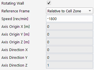
If the rotating domain contains static walls such as engine shrouds and bypass
splitters, these walls should be configured to have zero velocity in the
absolute reference frame. This can be done by setting Reference
Frame as and setting Speed
[rev/min] to 0 or with speed being the exact opposite of the domain
rotation rate. This is equivalent to setting walls as counter rotating in
FENSAP-ICE.
If the domain is rotating, then the walls can only have the same rotation axis and origin as the domain. Otherwise if the domain is fixed, it is possible to apply rotation to walls that are aligned with any axis and position.
For the steady state physics to be valid, walls set as must be axisymmetric.
Particles
Among all Particles type, the vapor model provides a wall boundary condition option that allows the walls to stay at 100% relative humidity and enables evaporation at these walls. To set this boundary condition check the Vapor Wet wall condition. This condition is usually not used in icing calculations. It is a useful feature to observe rates of evaporation and consequent vapor trail computed by the vapor transport PDE.
When the external reinjection model is enabled, the wall conditions involved in the reinjection process must be selected.
Note: It is required to select at least one wall for crystal bouncing.
Ice
Ice is computed over the walls of the computational domain. Two options are provided under Ice. The first Icing can be used to disable certain walls and exclude them from the computations. This could be used to enable an aircraft surface like the wing and/or the tail, while excluding the fuselage. The other option, , allows setting a heat flux on a wall to examine its impact on the ice accretion process. The latter could be used to quickly assess the amount of heat required to prevent ice formation, for instance.
Icing, just under Ice, is divided into five options:
This is the default setting under Icing and it allows the wall to be part of the computational domain for icing.
If selected, it will exclude the wall from icing calculations.
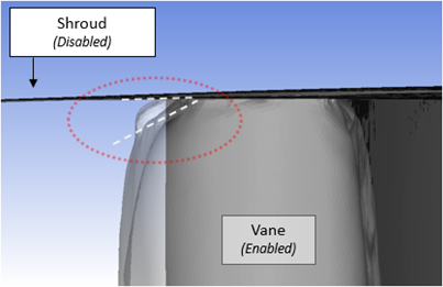
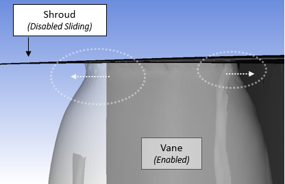
If selected, the wall will be included in the solution of surface water film continuity and energy equations, but ice displacement will be deactivated. The wall will act as a sliding support surface for adjoining surfaces that could displace and slide against it following a contact boundary condition.
If selected, it will remove this wall from the continuity and energy system while using it as a sliding support surface for adjoining ice accreting walls to slide against. A typical use of this option is the handling of hub and shroud walls of an engine stator while the blade accretes ice.
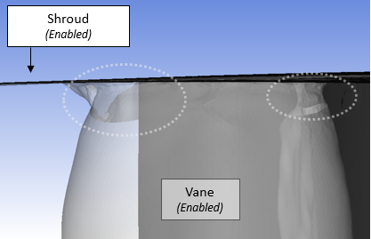
Note: The examples below illustrate how the options of , , and are affecting the results of icing calculations at the corner of the shroud and a guide vane attached to it. Figure 2.5: Wall Disabled shows the case where the shroud is disabled, and ice is only allowed to grow on the blade. This anchors the blade/shroud intersection nodes in place, and forces a tight concave space to form between the ice and the shroud. This can become a problem for multi-shot icing simulations if the remeshing algorithm cannot establish a good quality mesh at this region. Figure 2.6: Wall Disabled-Sliding shows the case where the shroud is set to , which allows the blade/shroud intersection nodes to slide across the shroud surface. This method has better success in remeshing during multi-shot icing simulations. Figure 2.7: Wall Enabled for Icing shows case where both the shroud and the blade are for icing calculations.
Sink
If selected, liquid water film will not be allowed to enter the wall and will act as an exit.
Built-in wall commands are available by right-clicking the Wall icon in the Outline View or by pressing on the buttons located at the bottom of the Wall properties window. Two commands are currently supported.
Temp. Adiabatic+10
Sets a temperature to the wall that is equal to the adiabatic stagnation temperature inside the Airflow settings panel, plus 10 K. In this manner, inside the Airflow submenu of the Wall properties panel, the Thermal Conditions will automatically switch to Temperature and the appropriate temperature will be shown next to Temperature [K].
Display
Displays the surface mesh of the wall selected in the Graphics window.
Pressure Outlet is currently the only outlet type supported by Fluent Icing.
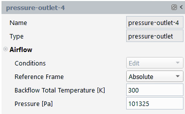
Three fields can be modified through the properties window of that boundary condition. The Reference Frame, Backflow Total Temperature [K] and Pressure [Pa]. Reference Frame allows the outlets to be defined relative to a cell zone motion or in absolute reference frame. This does not apply to fixed cell zones. However, if a rotating domain is defined, the outlet properties can be defined relative to the domain motion. Temperature then controls the backflow air properties when reversed flow occurs and pressure corresponds to the absolute pressure at the outlet, the absolute pressure is the result of adding the operating pressure to the gauge pressure in Fluent. The absolute pressure is equal to the static pressure variable used in FENSAP to specify a subsonic outlet.
Note: If more Pressure Outlet settings are required, for instance more settings are needed to define flow reversal conditions at the outlet, you can add them inside the original case file or through the Fluent session connected to Fluent Icing.
If turbomachinery domains such as fan and compressor rows are being simulated, Radial Equilibrium option is recommended for more realistic physics. This can be enabled in the Fluent workspace for that particular boundary, and in Fluent Icing the boundary condition should be set to . If Conditions is set to , it can be reverted to through the right-click menu.
Built-in outlet type commands are available by right-clicking the outlet type icon in the Outline View or by pressing on the buttons located at the bottom of the Outlet properties window. Two commands are currently supported.
Copies the Airflow settings into the Airflow submenu of the Outlet.
Displays the surface mesh of the Inlet type selected in the Graphics window.
In Solution, you will define the solver settings of your Fluent Icing simulation including monitoring, initialization and output files for each of its Fluent Icing modules (Airflow, Particles and Ice). These solver settings will allow you to conduct the five simulation scenarios mentioned in Setup as long as they have been properly selected in the Setup window.
The Solution window provides the multi-shot and general settings for all Fluent Icing modules.
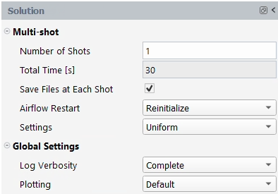
Multi-shot
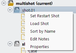
The Multi-shot menu under Solution is only available when all three solver types have been selected in the Setup window. See Multi-Shot. The total time of icing will be the sum of individual icing times set for each shot. By default, this is a uniform distribution and the per-shot time is entered in Solution → Ice. The shot time distribution can be modified by updating Settings from to . It is possible to restart from a step of a shot, by right-clicking an already partly or fully completed shot on the project panel and choosing :
Global Settings
This submenu sets the common output and monitoring settings of all Fluent Icing modules.
Log Verbosity
Controls the amount of convergence and execution information displayed (Minimal, Complete, Detailed) inside the Console window. Its content varies for each Fluent Icing module. Minimal is the default and will display a simplified convergence log (one line per iteration).
Plotting
Controls plotting of the residuals and any report set in the case file. Three options are supported.
Default will display the residual curves and any reports in the Plot window at every iteration.
Disabled will disable all plotting.
Fluent Icing components shown under Solution in the Outline View window are accompanied by an icon to their left. This icon reports if a solution file has been loaded or computed. The following table shows these icons.
| Airflow | Particles | Ice | |
|---|---|---|---|
| Solution not loaded or computed |
 |
 |
 |
| Solution loaded or computed |
 |  |
 |
To run a multi-shot calculation, first complete the set-up of all the Fluent Icing modules under Solution, then right-click the Solution icon in the Outline View and select .
The Airflow window under Solution allows the configuration of the airflow solver, monitor and output parameters. Depending on the Airflow solver selected in Setup, the Airflow window will show either Fluent or FENSAP parameters. Only steady-state airflow simulations are supported in Fluent Icing.
Fluent Airflow
In this window, the Number of Iterations to run a steady calculation is supported.
Time Integration
Select the solution control method used by Fluent:
: Uses the current settings from the case file.
: Sets the solution control to method with the option to set the time scale factor.
: Sets the solution control to method with the option to set the Courant Number.
: Sets the solution control to method with the option to set the Initial Courant Number, the Maximum Courant Number, First to High Order Blending [%] and the Explicit Under-Relaxation Factor. ( is only supported for the solver)
Note: is the recommended time integration scheme, with a time scale factor of 0.001 – 0.01. If using , it is recommended to not exceed a of 10.
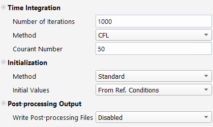
Initialization
Select the initialization method to be used by Fluent:
: Uses the current initialization settings from the case file.
: Performs the standard initialization by setting the Initial Values to the options below.
: The reference conditions defined in Setup → Airflow → Conditions.
: Values coming from an inlet boundary condition.
: User-defined initial values.
: Performs hybrid initialization.
Standard hybrid initialization of Fluent which computes an area weighted average of surface temperatures and applies it to the whole domain.
In Fluent Icing, this behavior is modified by patching the volume with the reference temperature after hybrid initialization is complete.
: Performs the FMG initialization with the specified FMG Courant Number.
Note: If FMG residuals are not decreasing, the initial solution will not be ideal to begin with. You can try lower values for the FMG Courant Number such as 0.2 to improve convergence.
See Fluent User's Guide in the Fluent User's Guide for more information about different initialization methods.
Moreover, it is also possible to specify the type solution output by selecting one of the three options inside Post-processing Output.
Default option. A Fluent solution (.dat, .dat.h5) is written and can be used to restart subsequent computations.
A Fluent solution and Post solution (.dat.post) are written.
Only a Post solution is written. No restart solution is written.
The Post solution file is used for post-processing purposes only. It can be read by the module, EnSight and CFD-Post. It does not contain all the information that it is necessary to resume a calculation and therefore it is considered to be lightweight to load when compared to a .dat or .dat.h5 file. When selecting or in Write Post-processing Files, several options are provided in order to define the content of the Post solution.
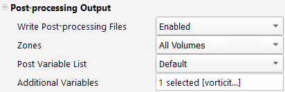
Zones
The post solution file is written using the full 3D domain.
Only selected surfaces (in the Surface Selection option below) are written to the file, leading to smaller file sizes but with no volumetric information.
Post Variable List
Select the list of variables written to the post file. Three options are available.
Velocity, Density, Temperature, Pressure, Heat Flux and Shear Stress fields are written.
Adds Mach Number, Viscosity, Thermal Conductivity, Cp, Wall Distance, Total Pressure, Total Temperature, Effective Viscosity and Pressure Coefficient to the post file.
Select the variables to be written to the post file from the list of variables that are available in Fluent post processing dataset.
An additional option, Roughness from Beading, is available in this window when an Ice solution with beads has been previously run and loaded to your Fluent Icing simulation.
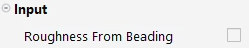
By enabling this option, the roughness distribution computed by the beads model will be applied as a boundary profile on all walls where the High roughness for Icing model has been enabled. The Roughness Height [m] of these walls will be updated to ICE3D Roughness file, which uses the ROUGHNESS boundary profile, the sand-grain beads profile, computed by Ice.
FENSAP Airflow Window
In this case, the Airflow window contains the most common steady-state solver and monitoring settings of the FENSAP airflow solver.
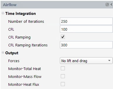
The Time Integration submenu allows the set-up of the
pseudo time step number, CFL, as well as the
Number of Iterations to use during the simulation. If
convergence problems are encountered, reduce the CFL or
activate the CFL Ramping Iterations option and specify a
number of CFL Ramping Iterations. This option gives access
to a mechanism that linearly increases the CFL number from
1, at the start of the simulation, to its full value
at the end of the CFL Ramping Iterations.
The Output submenu allows the creation of numbered solution files and of the most common monitoring variables to track in order to guarantee full convergence of the FENSAP solver.
Forces
By default, No lift and drag coefficients are outputted during the simulation. However, if Forces is set to Drag-Custom direction, the resultant lift, drag and moment coefficients (on all walls) will be monitored during the simulation. These aerodynamic coefficients are computed using the Conditions defined in Setup → Airflow and the following parameters.
Lift Axis
Provide the positive orientation of lift along the positive or negative X, Y and Z axis. FENSAP will obtain its true direction based on this information and the drag direction.
Drag – X, Drag – Y, Drag – Z
Provide the non-dimensional direction of drag in Cartesian coordinates.
Reference Area
Specify a reference area in m2 that is used to compute the aerodynamic coefficients.
Moment – X, Moment – Y, Moment – Z
Specify a point in the computational domain that will act as the moment center to compute the aerodynamic moment coefficient.
Monitor - Total Heat
If selected, monitors the total convective heat flux using all the walls of the computational domain.
Monitor -Mass Flow
If selected, monitors the mass inflow, outflow and deficit of air inside the computational domain.
Monitor -Heat Flux
If selected, monitors the total enthalpy inflow, outflow and deficit of the computational domain.
The Roughness from Beading is an additional option is available in this window when an Ice solution with beads has been previously run and loaded to your Fluent Icing simulation.
By enabling this option, the roughness distribution computed by the beads model will be applied as a boundary profile on all walls where the High roughness – Icing model has been enabled. The Roughness Height (m) of these walls will be updated to ICE3D Roughness file, which uses the ROUGHNESS boundary profile, sand-grain beads profile computed by Ice.
Airflow Commands
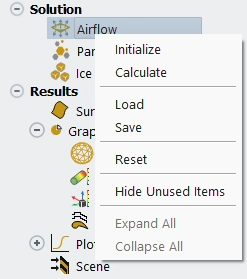
Built-in airflow commands are available by right-clicking the Airflow icon under Solution in the Outline View. The following commands are currently supported.
Executes an initialization of the airflow solver using the Initialization settings of Fluent. Initialize is not available for FENSAP. will also remove the green check mark next to the Airflow module icon and unbold the current airflow solution in the Project View.
Launches the simulation of the Airflow module. If a solution is loaded, the simulation will continue from that loaded solution. Otherwise, Calculate will first Initialize and then use this solution to solve the PDEs of the Airflow module.
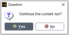
If a run has already been performed in the simulation, a window will appear asking if you would like to continue the current run. If , the calculation will continue in the current run folder. Once complete, a new solution file will overwrite the previous solution.
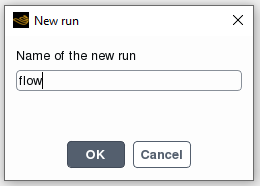
If is selected, a window appears asking for a Name of the new run. If is selected, a new run folder is created inside the simulation folder. This new folder contains a run settings file and all future solution files will be written in it.
If a solution is loaded in memory, the simulation will use it as an initial solution. Otherwise, will first Initialize and then compute the Airflow module.
Once the Airflow module begins to run, (running) will be displayed next to the Airflow module in the object tree. This state will change to (ended) if the Airflow module completes properly, or (interrupted) if the run is interrupted.
Interrupt
Stops the execution of the airflow solver at the end of the next iteration. The solution is kept in memory. This option is only available if Airflow is currently running.
Load
Loads an airflow solution file into memory.
Save
Saves the airflow solution that’s in memory to a file.
Reset
Removes the airflow solution from memory. will also remove the green check mark next to the Airflow icon and unbold the current Airflow solution in the Project View.
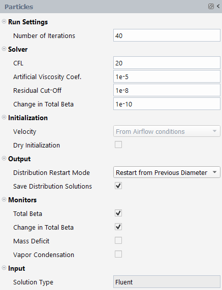
The Particles panel contains the most common steady-state solver, initialization and monitoring settings of the Fluent Icing Particles solver, DROP3D.
The Run Settings submenu allows the set-up of the Number of Iterations to conduct during the iterative simulation. A different Reinj. Number of Iterations is used to solve the reinjection loops.
The Solver submenu is divided into three points, the pseudo time step, the artificial viscosity and the convergence criteria.
CFL
The recommended values for the CFL range between
10and20. If convergence problems are encountered, reducing the CFL might help.Artificial Viscosity Coef.
The Particles module uses the Streamline upwind (SU) technique to stabilize the PDEs. This scheme is complemented with a user-set crosswind diffusion. Its default value is 1e-5 and has been extensively used in a large number of validation cases. In the case of structured grids, you can increase this value to 1e-4 if you experience oscillations of LWC within the shadow zone. Its impact to collection efficiency is generally minimal. Crosswind dissipation scales with mesh size, similar to the upwind scheme, and is lower with finer grids.
Residual Cut-Off
The Residual cut-off is the stopping criterion of the overall residual of the Particles governing equations. Lower the default value of 1e-8, especially if you are interested in capturing shadow zones.
Change in Total Beta
This parameter is the difference in total collection efficiency of all walls between two consecutive iterations. It is therefore a measure of convergence of the number of particles (droplets or crystals) that hit the walls of the computational domain. Lower the default value of 1e-10 if you see differences in collection efficiency between printouts.
Note: Both the Residual Cut-Off and Change in Total Beta thresholds can be increased a few orders to let DROP3D complete its runs quicker. Using 1e-6 and 1e-8 respectively can reduce the overall runtime significantly, while producing similar collection efficiency results. This is especially effective when running particle size distributions with large number of bins. You should verify the difference at least on a few sample cases before incorporating higher thresholds in your workflow.
The Initialization submenu allows the initialization of the particle concentration and particle velocity fields.
Velocity
Two initialization choices are offered for the velocity field.
From Airflow Conditions
If selected, the Speed and Direction inside of Setup → Airflow are used as the initial velocity of all types of particles at all nodes in the computational domain.
Cartesian components
If selected, specify the velocity components (X velocity [m/s], Y velocity [m/s] and Z velocity [m/s]) that will be assigned as the initial velocity for all particles inside the computational domain.
Dry Initialization
If selected, sets the particle concentration (LWC, ICC or Vapor Humidity) to zero everywhere inside the computational domain except at the inlet, where Particles boundary conditions are defined. Otherwise, the Particles concentration specified in Setup → Particles will be used to initialize the computational domain.
The Output submenu contains the following options:
Distribution Restart Mode
Select this option to initialize the solution fields of a droplet size with the results from the previously solved size. Depending on the case, this can decrease or increase the number of iterations needed to converge the droplet equations. For purely external flows, restarting from the previous diameter can be beneficial in reaching total beta convergence quicker. For flows with internal cavities, restarting from a previous solution may lead to some incorrect LWC that would have to be cleared with many iterations before reaching convergence. This is a case specific setting that should be studied before incorporating into the workflow of an analysis.
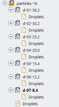
Save Distribution Solutions
Select this option if you would like to save all the solutions of a distribution simulation. The solutions will be numbered from 1 to the total number of particles sizes that define this distribution. The number 1 will be assigned to the largest particle size and the last number to the smallest particle size.
Note: This option is only available when a Particles or Crystal Distribution is selected under Setup → Particles → Droplets → Droplet Distribution, or Particles → Crystals → Crystal Distribution.
The folder structure for a particles distribution run will contain one result per diameter. The last result, not within a folder, is the combined solution obtained by mass-averaging the results of individual droplet size solutions.
The Monitors submenu allows the tracking of convergence of surface integral quantities such as collection efficiency, mass deficit and vapor condensation.
Total Beta
If selected, monitors the total collection efficiency computed on all walls of the computational domain.
Change in Total Beta
If selected, monitors the difference in total collection efficiency of all walls between two consecutive iterations.
Mass Deficit
If selected, monitors the mass inflow, outflow and deficit of particles inside the computational domain.
Vapor Condensation
If selected, monitors the total vapor condensation on all the walls of the computational domain.
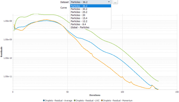
Note: In a particle distribution simulation, each particle size simulation is executed in sequence. The residuals graph is displayed at the end of the execution and will present a summary of the convergence of each calculation.
The residual graph is a combined plot of all the residual plots in a single sequence.
Particles Commands
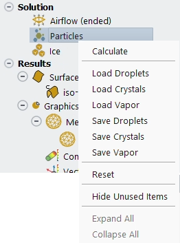
Built-in particles commands are available by right-clicking the Particles icon under Solution in the Outline View. The following commands are currently supported.
Calculate
Executes the Particles module.
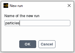
If a run has already been performed in the simulation, a window will appear asking if should continue in the current run folder. If is selected, the calculation will continue in the current run folder, and once complete, a new solution file will overwrite the previous solution.
If is selected, a window appears asking for a Name of the new run. If is selected, a new run folder is created inside the simulation folder. This new folder contains a run settings file and all future solution files will be written in it.
If a solution is loaded before is selected, the simulation will continue from that loaded solution. Otherwise, will first initialize and then solve Particles.
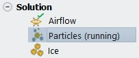
Once the Particles module begins to run, (running) will be displayed next to the Particles in the object tree. This state will change to (ended) if the Particles module completes properly, or (interrupted) if the run is interrupted.
Interrupt
Stops the execution of the particles solver at the end of the next iteration. The solution is kept in memory.
Load Droplets
Loads a particles droplets solution, with suffix .droplet, in memory.
Load Crystals
Loads a particles crystals solution, with suffix .crystal, in memory.
Load Vapor
Loads a particles vapor solution, with suffix .vapor, in memory.
Save Droplets
Saves only the water droplet solution files of your Particles simulation. This droplet solution file will contain the suffix .droplet.
Save Crystals
Saves only the ice crystal solution file of your Particles simulation. The crystal solution file will contain the suffix .crystal.
Save Vapor
Saves only the vapor solution file of your Particles simulation. The vapor solution file will contain the suffix .vapor.
Reset
Unloads the Particles solution from memory. will also remove the green check mark next the Particles icon and unbold the current Particles solution in the Project View.
This command enables you to hide unused graphics objects in the list For example, if only a Mesh object has been created, will reduce the list of objects under the dataset to show only the Meshes object. This can be helpful to reduce visual clutter when working with many datasets. You can select to reveal the unused hidden objects.
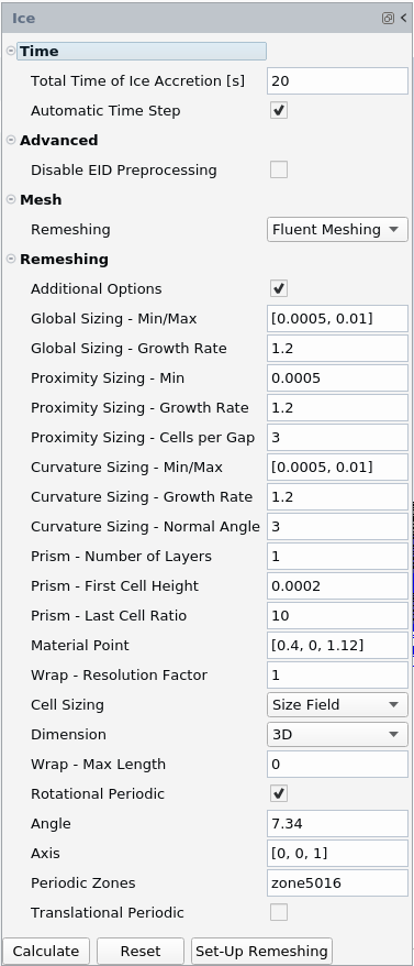
The Ice window contains the most common solver settings of ICE3D to obtain the new 3D computational domain over the ice shape.
The Time submenu allows the set-up of the Total Time of Ice Accretion [s] and the type of time step.
Total Time of Ice Accretion [s]
This is the icing time per shot.
Automatic Time Step
By default, this option is checked. The stable time step for an explicit time integration scheme depends on fluid speed and local mesh sizing. For time accurate problems, all control volumes must use the same time step. Automatic time stepping removes the guess work of specifying a stable time step. This option computes the optimal time step for each grid/film speed combination and largely reduces your computational time. If disabled, a Time step [s] option appears, where you can define a stable time step for the Ice simulation. For components with extremely small mesh size (turbomachinery blade tip section) the stable time step can be as low as 1e-6 seconds or less. If the time step is indeed too large for a certain mesh element, then a film flux limiting will be applied to explicitly retard the rate of water mass flow in that region to maintain stability.
This option is visible if is enabled through → → Icing. Extended Icing Data (EID) preprocessing extracts heat transfer coefficients (HTC) from a flow solution with adiabatic walls using a proprietary technology. In some scenarios related to adiabatic walls (see Boundary Conditions, Inlets, Airflow and Heat Flux Ice), the EID pre-processing will be executed automatically, prior to computing ice accretion. If this option is enabled, the EID preprocessing will be skipped. If the EID was already computed for the current airflow, the Ice simulation will use this EID solution. If EID does not exist, the Ice simulation will use the solution without the pre-processing, and heat transfer coefficients will be incorrect.
Note: The EID preprocessing is mandatory for simulations incorporating vapor transport.
The Mesh submenu allows the set-up of the numerical method to represent the volumetric mesh around the new ice shape. Two approaches are offered under Remeshing.
This option allows the update of the volumetric mesh by displacing/deforming the walls and the surrounding cells of the original mesh to account for the new ice shape. In this case, the mesh topology of the original mesh is preserved. However, even if this method is significantly faster than remeshing, not updating the grid topology has several limitations. Since the number of nodes remains constant, this method tends to coarsen the surface grid as ice accretes. In a multi-shot simulation, due to fixed mesh topology between shots, this method is not very effective in capturing complex glaze ice shapes. Due to these limitations, this approach often requires manual remeshing after a certain number of shots to maintain appropriate mesh and solution quality.
Using Fluent Meshing, this option allows the automatic reconstruction of a volumetric unstructured mesh, composed of tetrahedra and prisms, around the iced surface while preserving the other boundaries of the original mesh. A surface mesh is first obtained around the new iced surface using a wrapping approach. Then, a volumetric mesh is constructed around the wrapped surface. Therefore, when this option is selected, wrapping and remeshing parameters are available under the Remeshing submenu and control the surface mesh resolution and the mesh quality of the volumetric mesh around the iced surface. To activate remeshing with Fluent Meshing, click at the bottom of the Ice panel.
Note:
Wrapping and remeshing parameters set in the Remeshing submenu remained fixed when conducting multi-shot calculations. As ice builds up, the mesh size at each shot increases and more computing time and memory is required to solve the airflow, particle, and ice solvers. Special attention should be given to these meshing parameters to obtain cost-effective multi-shot solutions at each shot. To take into account the increase in computing cost per shot, one could gradually increase the number of cores per shot. This can be done by stopping and restarting your multi-shot calculations. Refer to Multi-Shot. Alternatively, one could start a multi-shot simulation with a larger number of cores than would be typically required. Furthermore, different airflow solvers may require different mesh settings to produce mesh independent results, and these settings can be case specific. Therefore, restarting multi-shot calculations will also allow you to tailor the convergence settings of the airflow and droplet solvers to improve the quality and the precision of the overall multi-shot simulation.
Walls should be separated into different zones at corners or joints. Doing so will ensure that sharp edges of the geometrical model will be preserved after wrapping. For example, if the tip cap of a wing is placed in the same boundary family as the rest of the wing, the corners will be smoothed during the wrapping operation, which should be avoided.
The Remeshing submenu is visible when is selected in the Mesh submenu. This submenu allows the set-up of the wrapping and meshing parameters to generate the mesh around the iced surface. Fluent Meshing performs three main steps, surface meshing, volume meshing, and 2.5D extrusion (optional), during mesh generation. The list below links each Fluent Meshing parameter to one of these steps.
Surface Meshing
Material Point
Global Sizing - Min/Max and Growth Rate)
Curvature/Proximity Sizing (Min/Max, Normal Angle, Cells per Gap, and Growth Rate)
Wrap – Resolution factor
Wrap – Max Length (if applicable)
Periodic – Translational/Rotational (if applicable)
Volume Meshing
Prisms (First Cell Height, Last Cell Ratio, and Number of Layers)
The recommended values for Prism - First Cell Height and Prism - Last Cell Ratio are 1e-6 meters (1 micron) and 10 (percent) respectively.
These values are used for ice shape validations.
Increasing the number of layers increases the accuracy of the boundary layer and heat transfer coefficients. For most problems, a layer count between 20-30 should lead to accurate results. If unsure, a parametric study could be done to check prism layer mesh convergence and multishot ice shapes for a particular problem.
Cell Sizing (, or )
2.5D Extrusion (if applicable)
Extrusion – Z Thickness
Note: Fluent Meshing will use the parameters of the surface meshing step to compute a virtual throughout the domain before generating the wrapped surface mesh.
The figure below shows a layout where these meshing parameters are applied inside the computational domain.
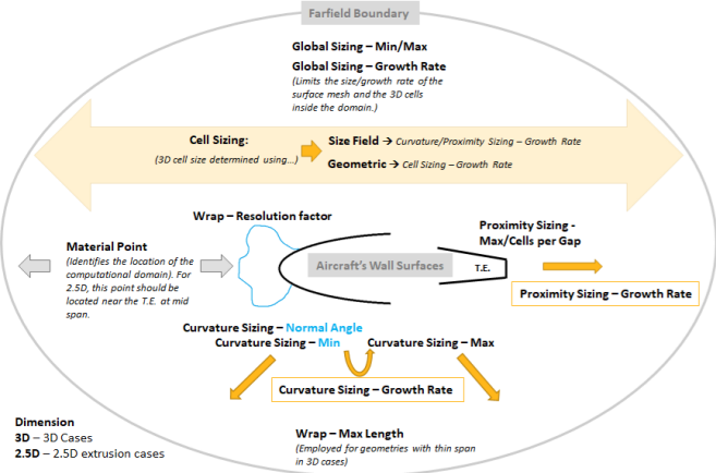
Below is a brief description of the parameters that are exposed in Fluent Icing.
If a parameter requires more than one entry, separate each entry by a comma and
add brackets around them (example: [x, y, z]). For more
information regarding these parameters, consult Size Functions and Scoped Sizing in the Fluent User's Guide.
Allows you to control the following expert parameters:
Proximity Sizing – Growth Rate
Proximity Sizing – Cells per Gap
Curvature Sizing – Normal Angle
Wrap – Resolution Factor
Cell Sizing
Cell Sizing – Growth Rate
Wrap – Max Length
Global Sizing – Min/Max
Minimum and maximum global cell size of triangles or tetrahedra used during wrapping and mesh creation.
Global Sizing – Growth Rate
Growth rate of triangles or tetrahedra between the minimum and maximum cell size inside the computational domain used during wrapping and mesh creation.
Proximity Sizing – Min
Minimum cell size used in the proximity of the surface. This is used for wrapping and surface mesh creation.
Proximity Sizing – Growth Rate
Growth rate of cell size in the proximity of the surface. This is used for wrapping and surface mesh creation.
Proximity Sizing – Cells per Gap
Number of cells are filled between two proximal surfaces. This parameter is useful when you have a blunt trailing edge in your geometry. It will assign the given number of mesh cells over the blunt surface of the trailing edge. The figure below shows four Cells per Gap assigned to a wing’s blunt trailing edge surface.
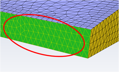
It’s also applied to close some small gaps inside the complex iced surface.
Curvature Sizing – Min/Max
Minimum and maximum cell size used to capture the curvature of wall surfaces. This is used for wrapping and surface mesh creation.
Curvature Sizing – Growth Rate
Growth rate of the cell size used to capture the curvature of wall surfaces. This is used for wrapping and surface mesh creation.
Curvature Sizing – Normal Angle
Difference between the normal angle of two neighboring wall cells. This value is used to identify curved locations where the minimum cell size should be applied. The default value of 5 is suitable for most icing simulations. A range between 2 to 10 is recommended.
Note: The Curvature Sizing – Min and Normal Angle are key factors to properly represent the computed ice shape throughout multi-shot simulations.
Prism – Number of Layers
Number of prism layers to generate around wall boundaries.
Prism – First Cell Height
Height of the first prism layer just above the wall boundaries.
Prism – Last Cell Ratio
The ratio of the top layer prism height as a percent of the tetrahedron height just above. Default Fluent Meshing value for this parameter is 40%. However, for aerodynamic problems and ice shape validations, the recommended value is 10%.
Material Point
A point located in the area where you would like to create the volume mesh. Specify its location using cartesian coordinates, example [x, y, z]. Fluent Meshing will use the material point to define the domain, around which a surface mesh will be created and 3D cells will be filled. In the case of 2.5D meshes, the material point must be defined at a location close to the trailing edge and at the middle of the z-span.
Wrap – Resolution Factor
Controls the resolution of the surface during wrapping. A value of 0 will capture all features present in the ice shape. A higher value will smooth discontinuities present in the ice shape produced by ICE3D. A default value of 0.75 was selected based on 3D validation cases. Reducing the resolution factor will cause wrapping to use a finer background mesh for feature capturing, which will increase the time and memory cost of the wrapping operation.
Cell Sizing
This parameter is used to generate 3D cells inside the domain. It has two sub options, and . These options determine how these 3D cells grow from the existing surface mesh to the outer boundaries of the domain.
When this option is selected, Fluent Meshing will use the existing virtual to determine the size of the cells inside the domain.
When this option is selected, Fluent Meshing will use the existing surface mesh, ignoring the virtual , together with the Cell Sizing – Growth Rate to determine the size of the cells inside the domain.
Note: The Cell Sizing → option with Growth Rate of 1.2 is set by default. To modify these values, enable .
Cell Sizing – Growth Rate
Controls the cells growth from the existing surface mesh to the outer boundaries of the domain.
Dimension
Specify if the original mesh is a full 3D mesh or a 2.5D mesh. A 2.5D mesh has a span of one cell. When 2.5D is selected, the remeshing process has the following requirements for the original mesh:
The span of the geometry must be placed along the Z-axis;
The span direction must be Z+ and the source symm plane must be placed at Z = 0;
Paired symmetry-z planes must be defined. Therefore, individual symmetry-z BC must be merged into one symmetry-z BC as “symmetry” type. The same goes for translational periodic planes.
The material point must be defined at a location that is close to the trailing edge and at half-span.
The original 2.5D mesh can be any of the following cases:
2.5D regular (farfield + Z-symmetry + one airfoil element)
2.5D + multi-element airfoil
2.5D + multiple symm planes
2.5D + translational periodicity in an off-symm direction
Note: If the original mesh has additional symmetry or translational periodic planes in X, Y, or any other direction that do not represent the span of the geometry, these planes can remain unpaired.
Periodicity
Respectively, select , or if the original mesh contains no periodicity, translational periodicity or rotational periodicity. If or is selected, extra parameters will appear under and should be specified.
If
Translation
The translational periodic vector in cartesian system [vx, vy, vz] m.
Periodic Zones
The Zone name of the translational periodic surfaces in the original mesh.
If
Angle
The rotational periodic angle of the original mesh, which is the rotation angle between the periodic and its shadow zone.
Axis
The axis of the periodic zone of the original mesh in cartesian system [vx, vy, vz] m.
Note: Periodic center will be taken as 0, 0, 0, since the rotation axis has to be one of the primary coordinates.
Periodic Zones
The Zone name of the rotational periodic surfaces in the original mesh.
Note:
Paired periodic zones that shared the same vector or rotational Angle/Axis should be merged into one BC zone.
Zone5998 and Zone5999 are reserved zone names of Fluent Icing and are used during the remeshing process. Avoid employing these names in the original mesh.
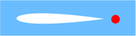
After completing an icing calculation or loading an icing solution into
Fluent Icing, the following icon  will be displayed next to Solution
→ Ice in the Outline
View.
will be displayed next to Solution
→ Ice in the Outline
View.
Note: If the icing solver step does not result in ice formation, a warning message will appear inside the log panel of Fluent Icing. This will not stop a multi-shot simulation.
The Shedding Outputs submenu will be visible if
Ice Shedding is enabled in the
Setup → Ice panel. In this
case, the Shedding Interval [s] determines when the
single-shot ice shape will be analyzed for stress distribution and crack
propagation. Stress analysis is a relatively expensive process and does not need
to be done at every ice accretion time step. At each shedding interval, the
single-shot ice shape will be filled with a volume mesh that uses the existing
surface mesh topology, and will be sent to the intrinsic solid mechanics solver
of the Ice module. Crack propagation iterations will take place, and if there
are any ice fragments detected to break off, they will be removed from the ice
shape as well as the Ice Growth solution field.
The numbered solution output will write a different
ice.grid and swimsol file for each
interval, numbered with the interval count.
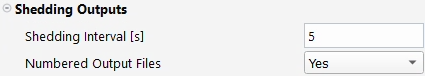
Output files for a shedding analysis will not be readily visible in the file tree view under the Project View. To see these files, you can right-click Name under Project View and check Show all files.
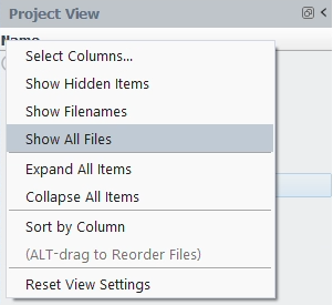
Example 2.1: List of Files That Will Be Saved
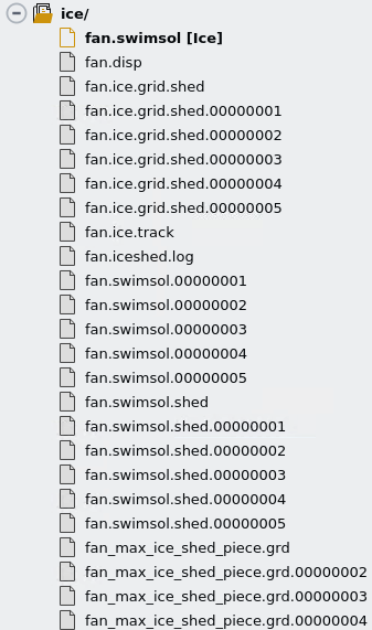
*.shed* files are the FENSAP format ice grid files after the ice shape has been retracted to account for shedding.
*.iceshed.log file contains information about the fragmented ice shapes, mass loss, etc. per ice shedding interval.
*.swimsol.shed* files contain the
Ice Growthfield that is modified by removing the shed ice mass from each mesh point. Additional solution fields are provided that are relevant to the ice shedding process, like fragment ID, principal stresses, shed ice mass, etc.*max_ice_shed_piece* is the FENSAP format mesh file for the largest ice fragment that shed at each shedding analysis interval.
Currently, the Fluent Icing user interface does not provide a direct method to view these additional files. You can do so by navigating to the run directory and launching FENSAP-ICE → Viewmerical with the grid and solution file names.
Ice Commands
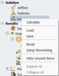
Some built-in commands are available by right-clicking the Ice icon under Solution in the Outline View.
Calculate
Executes the Ice module.
After clicking , a window appears asking for a Name of the new run. If is selected, a new run folder is created inside the simulation folder. This new folder contains a run settings file and all future solution files will be written in it.
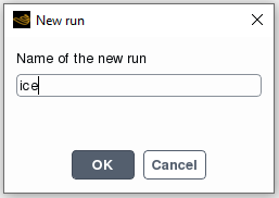
will execute the Ice module using null values for ice accretion rate and water film height and adiabatic wall temperatures as initial quantities.
Once Ice begins to run, (running) will be displayed next to Ice in the object tree. This state will change to (ended) if Ice completes properly, or (interrupted) if the run is interrupted.
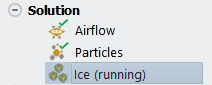
Once ice simulation is conducted, the Update grid becomes available. This allows the creation of a 3D mesh by displacing/deforming the walls and the surrounding cells of the original mesh to account for the new ice shape. The next step in this process would be to run the airflow solver on this new grid to obtain the local airflow conditions and properties around the new ice shape. Further calculations (particles and ice) should then be obtained on this updated mesh. The case file will then contain the new ice shape and a would be required to avoid overwriting the original un-iced case file.
Note: In a multi-shot simulation, the iced surface and the volume mesh surrounding it is updated at the end of each shot using Lagrangian displacement or complete remeshing.
Stops the execution of the ice solver at the end of the next iteration. The solution is kept in memory.
Loads an Ice solution in memory. Ice restart capabilities are not supported.
Saves all Ice solution files of your simulation. The name of these files contain the suffixes ice.grid, .map.grid and .swimsol. For more information regarding these output files, consult Results.
Unloads the Ice solution. Reset will also remove the green check mark next the Ice component icon and un-Bold the text of the current Ice solution in the Project View.
Activates remeshing with Fluent Meshing.
A multi-shot run executes the three solvers (Airflow, Particles, Ice) in sequence.
This option allows the control of the number of quasi-steady shots to simulate and saving output files of Airflow, Particles and Ice at each shot, if needed.
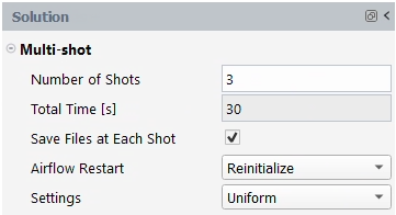
Number of Shots
This option allows you to control the number of quasi-steady shots to simulate, which is one instance of Airflow – Particles – Ice calculation. Grid displacement is executed at the end of each shot and used as an input for the next step.
Save Files at Each Shot
Enabled by default, all the solution files for each solver step (Airflow, Particles, Ice and Mesh Update are saved to the run folder.
If disabled, only the Ice solution files are saved at each shot and can be post-processed. The final Case file (mesh with the final ice shape using grid displacement or remeshing) is also saved. If is disabled, the Restart Shot feature cannot be used, as the required restart files are not present.
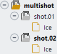
Airflow Restart
This option controls the initial solution of the airflow at each shot. Two options are available, and . will use the default settings of the initial case file at each shot. will use the interpolated airflow solution of the previous shot as the initial airflow solution for the next shot.
Note: Restarting from an interpolated solution demands large amounts of free memory in addition to what’s already taken by the parallel Fluent processes. Insufficient memory will lead to error state at the time of processing the interpolation file.
Settings
This option allows the control of the number of iterations for the first shot. Depending on the simulation at hand and the type of initial solutions specified in Airflow Restart, it is possible that the first shot requires more or less iterations than the next shots. Two options are available: and .
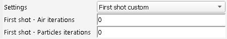
Uniform will use the same amount of solver iterations across all shots. First shot custom allows for a different number of iterations in the first shot. The remaining shots will use the settings from the Solution panels.
Multi-Shot Commands
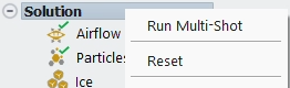
Built-in multi-shot commands are available by right-clicking the Solution icon in the Outline View. The following commands are currently supported.
Executes the multi-shot sequence for Number of Shots. The grid file is displaced with the ice shape at the end of each shot.
The current state of the execution is displayed in the Outline View. While the multi-shot calculation is running, the currently running shot step will be displayed next to Solution, and (running) will be displayed next to the module that is currently running, as shown below.
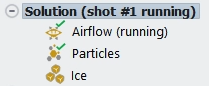
Once all shots are complete, the final shot number will be displayed as ended, and multi-shot complete will be specified.
After the final shot has ended, the grid file of the first shot will be re-loaded, and will be specified next to Solution, as shown below.
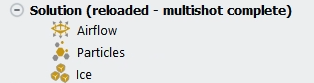
After a multi-shot simulation completes successfully, the shot 1 grid is always re-loaded to make sure you will start from the initial grid if you continue to run another multi-shot computation.
Note: In addition to using the command, A multi-shot sequence can be manually set by executing the Airflow, Particles, Ice solvers one after the other. In this case, do not forget to click in Solution → Ice to account for ice shape updates within the 3D grid and, if the Beading model is used, activate Roughness from beading in Solution → Airflow to consider the impact of the sand-grain roughness produced by the beads onto the airflow.
Stops the multi-shot computation at the current step. The solution is saved at the current state. This option is only available when the multi-shot simulation is running.
After interrupting a multi-shot computation, the loaded grid and solutions will remain at their present position. Hence, if the grid has already been displaced to account for the growth of ice, that grid will currently be loaded. At this point, if you would like to run another simulation, in order to make sure you start from the initial clean grid for the new run, you must use the command to load the initial grid in memory.
Resets and unloads all solutions. This is equivalent to executing on each Airflow, Particles and Ice tree nodes. The grid that is currently loaded in memory is not reset by this operation. will also remove the green check mark next to the Airflow, Particles, and Ice module icons and unbold the text of the current Airflow, Particles and Ice solutions in the Project View.
Reloads the initial grid, and resets and unloads all solutions. This is equivalent to executing the Load command on the out.cas(.h5) of the current multishot run, as well as executing on each Airflow, Particles and Ice tree nodes. will also remove the green check mark next to the Airflow, Particles, and Ice icons and unbold the text of the current Airflow, Particles and Ice solutions in the Project View.
Note: The multi-shot morphs the grid with the iced wall surfaces at each shot. The Reset operation will reset solutions, but will not load the original grid. To revert to the initial state that you had at the beginning of the multi-shot run, use the Reset multishot command. Alternatively, to revert to a specific shot, right-click the appropriate case file and select , or use the File → Open menu and select the appropriate case file to load. Loading a case file will also load its settings in Fluent Icing.
Multi-shot Restart
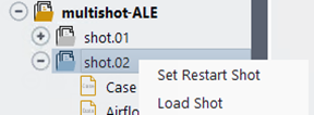
It is possible to restart an interrupted multi-shot run from a specific step. To accomplish this,
In the Project View, right-click the shot of interest and select .
A restart step within that shot can be selected from the Solution panel. The active shot is also displayed in bold in the Project View.
Note: This is not available for computations executed with disabled.
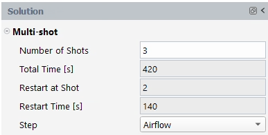
Restart at Shot
Displays the selected shot for the restart.
Restart Time [s]
Indicates the icing time reached at the start of that shot.
Step
Selects the solver step at which to resume the computation (Airflow, Particles, Ice, Mesh Update).
Once the step to restart the calculations has been selected, use the command to continue the computation.
Note: When restarting a multi-shot calculation, it is strongly recommended to keep physical models, conditions, and boundary conditions unchanged. All parameters that are exposed inside Setup in the Outline View of Fluent Icing should remain constant when restarting a multi-shot calculation, otherwise these new simulations will produce results that will be different than the uninterrupted calculation. Only parameters that are exposed inside Solution should be modified as they only affect the convergence, stability and mesh refinement (remeshing) of simulations. Moreover, the original settings of the multi-shot run can be loaded from the Project View by right-clicking the respective multi-shot run and then selecting .
is not used for multishot restarts. Instead, it is used to load all of the solutions from that shot (Case file, Airflow solution, Particles and Ice solutions) into Fluent Icing. Post-processing tools of Fluent can be used on that loaded solution. To save that new case state in the project and reuse it in a simulation, use (to save in the current simulation) or Duplicate Simulation (to save in a new simulation) since would update and overwrite the original case file with the new mesh state.
The CHT section defines the control and output of the CHT anti-icing simulation.
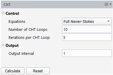
Equations
This delineates the system of equations to be tackled by the Fluent solver. The option incorporates momentum, turbulence, and energy equations, whereas the option exclusively solves the energy equation while maintaining the stagnation of the momentum and turbulence equations. This approach can lead to a reduction in computational time, operating under the assumption that the airflow's momentum and turbulence solutions remain relatively unchanged with the introduction of ice cooling and anti-icing heat supply. will remain the original settings from the case file.
Number of CHT Loops
This is the total number of CHT loops. The calculation will terminate once it reaches the total number of loops. During a CHT loop, the model equations are solved and thermal boundary conditions are exchanged and updated between the domains. At the end of each CHT loop, Fluent’s airflow and icing solver will exchange information at the icing surfaces.
Iterations per CHT Loop
This represents the upper limit of solver iterations within each CHT loop. The computation can advance to the subsequent CHT loop provided that the residual meets the desired convergence threshold, even if the iteration count doesn't reach the maximum threshold.
Output Interval
This denotes the frequency at which the CHT solution is written. The CHT solution encompasses a collection of solutions involving airflow and icing.
Note: Anti-icing CHT is a steady-state solution method where the model inputs heating power and flow and droplet boundary conditions are kept constant. The solution is expected to reach a converged state. The rate of convergence and success is a combined function of the CFL number or the pseudo time step setting in Fluent, the solver iterations per CHT loop and the total number of CHT loops. Providing a best practice on these individual settings is not possible since the performance will be case specific. Ensure the residuals sufficiently drop during each CHT loop, with a proper combination of solver time stepping and iterations per CHT loop. For some problems, using only 1 iteration per CHT loop could theoretically work if the CFL number is low enough.
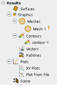
The Results branch in the Outline View provides access to the core Fluent post-processing options as presented in the Remote Visualization Client and offers the same options as in Fluent’s user interface.
Note: All post-processing performed using the options available in Outline View → Results, or in the top ribbon, Results → Quick-View, are performed using the solutions currently loaded in memory. The command in the Project View loads the Post-Analysis feature and allows to load file sequences and to combine complex scenes with multiple datasets, see Post-Analysis (Beta) in Fluent Icing. Alternately all solution files can be post processed using Viewmerical, CFD-Post or EnSight by right-clicking the file in Project View and selecting the appropriate option, as described in Using the Project View to Interact with Fluent Icing Simulations.
The different object types offered under Results → Graphics are:
Surfaces
Create cutting planes or other post-processing surfaces from the mesh.
Meshes
Displays the current mesh surfaces.
Contours
Displays contours of solution fields over surfaces. The results of Fluent Icing are listed in the Icing variable category. The list of available Fluent Icing fields will depend on the solution files currently loaded (airflow, droplets, crystals, vapor, ice). All Fluent Icing fields are solutions defined at the nodes.
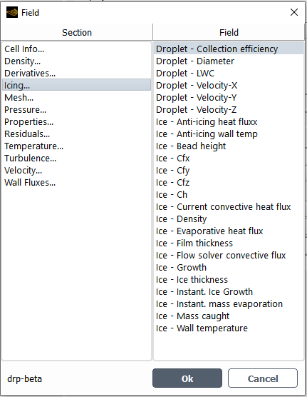
Vectors
Displays vector solution fields in the entire computational domain or on selected surfaces. Only supported for Fluent airflow solution variables. Use Viewmerical or CFD-Post to post-process FENSAP Particles and Ice vector solutions.
Pathlines
Displays flow and particle paths within the computational domain. Only supported for Fluent airflow solution variables. Use CFD-Post or EnSight to post-process Particles and Ice pathlines.
Volume Renderings
Displays all 3D elements at once, drawing each element semi-transparently according to the value of a variable using user-selected x, y, and z dimensions to control the number of elements passed up to the client.
Periodic Instances
Creates repeating copies, or periodic instances, of selected boundaries in the workspace.
Mirror Planes
Create 2D XY plots of your results for analyzing one variable with respect to another variable. For more details on Mirror Planes, see Mirror Planes.
Some mesh and common Fluent Icing fields can be viewed quickly by using Quick-View. See Quick-View for more details.
To create and display a new graphic object:
Right-click the object type of interest (Meshes, Contours, etc.), and select
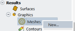
or use the command buttons in the Results window of the Ribbon.
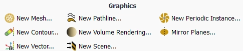
In the mesh-1 window, set up the graphical object options, and choose the Surfaces to display. A description on how to generate these object types can be found inside Basic Graphics Generation.
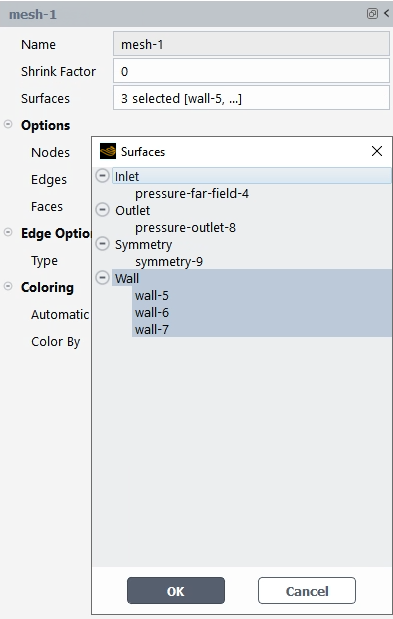
Select Display in the contextual menu of the new object to output the result in the Graphics window.
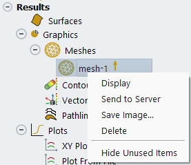
Scenes
Combine multiple graphical objects (mesh, contours, etc.) in the graphic window.
Quick-View allows you to easily output the most common Fluent Icing fields on walls and other boundary surfaces. A Fit to Window view is applied in all cases by default.
Note: Quick-View will use the solution data of the currently selected Fluent case file. To output the solution of another Fluent case within the Outline View, select the desired case before running Quick-View.
Three object types are supported in Quick-View.
Mesh
Displays the boundary surface meshes of computational domain (inlet, outlet, wall, symmetry)
Only the wall surfaces are displayed.
Opens Viewmerical with the mesh currently loaded in memory.
Opens CFD-Post with the mesh currently loaded in memory.
Contour
Airflow
FENSAP/Fluent
Temperature (Walls)
Displays the temperature distribution on all walls.
Heat flux (Walls)
Displays the convective heat flux distribution on all walls.
Velocity Magnitude
Displays the airflow speed on all boundary surfaces.
FENSAP format only
Opens Viewmerical with the mesh and the airflow solution currently loaded in memory.
Opens CFD-Post with the mesh and the airflow solution currently loaded in memory.
Particles
Droplets / Crystals
Collection Efficiency (Walls)
Displays the collection efficiency of the droplets or crystals on all walls.
LWC / ICC
Displays the LWC or ICC on all boundary surfaces.
Opens Viewmerical with the mesh and the droplet or crystal solution currently loaded in memory.
Opens CFD-Post with the mesh and the droplet or crystal solution currently loaded in memory.
Opens EnSight with the mesh and the droplet or crystal solution currently loaded in memory.
Vapor
Vapor Concentration
Displays vapor concentration on all boundary surfaces.
Vapor Condensation
Displays vapor condensation on all walls.
Opens Viewmerical with the mesh and the vapor solution currently loaded in memory.
Opens CFD-Post with the mesh and the vapor solution currently loaded in memory.
Opens EnSight with the mesh and the vapor solution currently loaded in memory.
Ice
Ice Thickness
Displays the ice thickness on all walls.
Opens Viewmerical with the surface mesh (map.grid) and the ice solution (swimsol) currently loaded in memory.
Opens CFD-Post with the surface mesh (map.grid) and the ice solution (swimsol) currently loaded in memory.
Opens EnSight with the surface mesh (map.grid) and the ice solution (swimsol) currently loaded in memory.
Ice Cover
Ice Cover – Viewmerical / CFD-Post
Displays the 3D ice shape over the original surface. In the case of CFD-Post, the display of the ice shape is done by executing the Ice Cover – 3D-View icing macro. Once in CFD-Post, Ice Cover – 2D-Plot icing macro can be also enabled.
Displays the 3D ice shapes obtained during each shot over the original surface. The display of all ice shapes is done by executing the Ice Cover – 3D-View icing macro. Once in CFD-Post, Ice Cover – 2D-Plot icing macro can be also enabled.
A single quick-view item can be displayed at a time in the Graphics window and will replace the previous item displayed. To store multiple items in different windows, use the Results node in the Outline View as detailed in Results.
Selecting a Quick-View will reset the current view. To update the current Quick-View with the latest solution, use the Display command from the contextual menu in the Outline View.
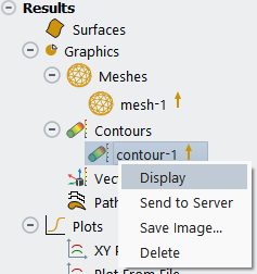
For more information regarding Viewmerical and CFD-Post, consult Post Processing with Viewmerical and CFD-Post from Fluent Icing.