


In Ansys Fluent, two solver technologies are available:
pressure-based
density-based
Both solvers can be used for a broad range of flows, but in some cases one formulation may perform better (that is, yield a solution more quickly or resolve certain flow features better) than the other. The pressure-based and density-based approaches differ in the way that the continuity, momentum, and (where appropriate) energy and species equations are solved, as described in Overview of Flow Solvers in the Theory Guide.
The pressure-based solver traditionally has been used for incompressible and mildly compressible flows. The density-based approach, on the other hand, was originally designed for high-speed compressible flows. Both approaches are now applicable to a broad range of flows (from incompressible to highly compressible), but the origins of the density-based formulation may give it an accuracy (that is shock resolution) advantage over the pressure-based solver for high-speed compressible flows.
Two formulations exist under the density-based solver: implicit and explicit. The density-based explicit and implicit formulations solve the equations for additional scalars (for example, turbulence or radiation quantities) sequentially. The implicit and explicit density-based formulations differ in the way that they linearize the coupled equations. For more details about the solver formulations, see Overview of Flow Solvers in the Theory Guide.
Due to broader stability characteristics of the implicit formulation, a converged steady-state solution can be obtained much faster using the implicit formulation rather than the explicit formulation. However, the implicit formulation requires more memory than the explicit formulation.
Two algorithms also exist under the pressure-based solver in Ansys Fluent: a segregated algorithm and a coupled algorithm. In the segregated algorithm the governing equations are solved sequentially, segregated from one another, while in the coupled algorithm the momentum equations and the pressure-based continuity equation are solved in a coupled manner. In general, the coupled algorithm significantly improves the convergence speed over the segregated algorithm, however, the memory requirement for the coupled algorithm is more than the segregated algorithm.
When selecting a solver and an algorithm you must consider the following issues:
The model availability for a given solver.
Solver performance for the given flow conditions.
The size of the mesh under consideration and the available memory on your machine. This issue could be an important factor in deciding whether to use an explicit or implicit formulation when the density-based solver is selected, or to use a segregated or coupled algorithm when the pressure-based solver is selected.
The following two lists highlight the model availability for each solver:
Important: Note that the pressure-based solver provides several physical models or features that are not available with the density-based solver:
Cavitation model
Volume-of-fluid (VOF) model
Multiphase mixture model
Eulerian multiphase model
Non-premixed combustion model
Premixed combustion model
Partially premixed combustion model
Composition PDF transport model
Soot model
Rosseland radiation model
Melting/solidification model
Shell conduction model
Floating operating pressure
Fixed variable option
Physical velocity formulation for porous media
Specified mass flow rate for streamwise periodic flow
The following features are available with the density-based solver, but not with the pressure-based solver:
Wet steam multiphase model
For additional information, see the following sections:
To choose one of the solvers, you will use the General Task Page (Figure 36.1: The General Task Page).
![]() Setup →
Setup → ![]() General
General
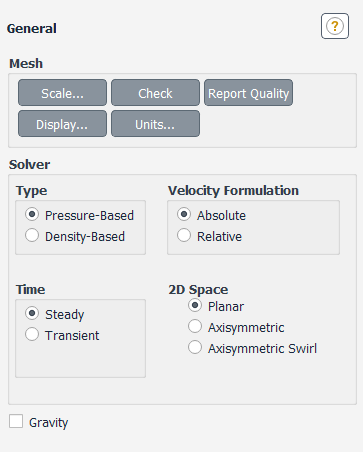
To use the pressure-based solver, retain the default selection of Pressure-Based under Solver.
To use the density-based solver, select Density-Based under Solver.
After you have defined your model and specified which solver you want to use, you are ready to run the solver. The following steps outline a general procedure you can follow:
(pressure-based solver only) Select the pressure-velocity coupling method (see Choosing the Pressure-Velocity Coupling Method ).
Choose the spatial discretization scheme and, for the pressure-based solver, the pressure interpolation scheme (see Choosing the Spatial Discretization Scheme).
(pressure-based solver only) Select the porous media velocity method (see Porous Media Conditions).
Select how you want the derivatives to be evaluated by choosing a gradient option (see Evaluation of Gradients and Derivatives in the Theory Guide).
Set the under-relaxation factors (see Setting Under-Relaxation Factors).
(density-based explicit formulation only) Set up the FAS multigrid (see Turning On FAS Multigrid).
Make any additional modifications to the solver settings that are suggested in the chapters or sections that describe the models you are using.
Enable the appropriate solution monitors (see Monitoring Solution Convergence).
Initialize the solution (see Initializing the Solution).
Start calculating (see Performing Steady-State Calculations for steady-state calculations, or Performing Time-Dependent Calculations for time-dependent calculations).
If you have convergence trouble, try one of the methods discussed in Convergence and Stability.
The default settings for the first three items listed above are suitable for most problems and need not be changed. The following sections outline how these and other solution parameters can be changed, and when you may want to change them.