


Many of the icing features and settings can be accessed and changed through the Console window, using python commands.
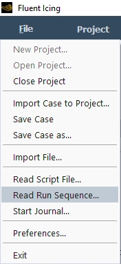
Many of the commands and settings present in the Fluent Icing panels can be recorded using python commands from the → menu. These journal files can also be executed through the → menu.
Python Console & Operations
The Console window at the bottom right corner of Fluent Icing allows you to enter commands interactively. The following sections describe commands available in the python console
dir() and the command/attribute list
dir()
Display the list of global commands and top-level objects.
'AddSession', 'Project', 'ReadScriptFile', 'Sim', 'StartTranscript', 'StopTranscript', 'csim', 'currentSimulation'
dir(object)
Display the list of commands & attributes of the object.
Example 2.2: Entering Commands Interactively
(Assuming test1.cas is already loaded)
dir(Sim[“case_file”])
'Case', 'Connect', 'ConnectionInfo', 'IcingSimulation', 'StartServer'
r = currentSimulation()
A temporary variable can be used to simplify command lines.
dir(r.Case.App.Particles)
'Crystals', 'Droplets', 'Model', 'Type', 'Vapor'
dir(r.Case.App.Particles.Droplets.Particles.Droplets.Conditions)
' Appendix', 'Diameter', 'LWC', 'SLDFlag', 'WaterDensity'
Accessing/Changing Values
The () operator will return the current value of the
attribute.
r.Case.App.Particles.Conditions.LWC()
Result: 0.001
r.Case.App.Particles.Conditions.LWC = 0.00344
Commands
If an item listed in dir() is a verb, it is a command.
For example
r.Case.App.Solution.AirflowRun.Initialize()
Sample Script
c = csim()

# Droplets: Configure
c.Particles.Droplets.Conditions.Diameter = 16
c.Solution.ParticlesRun.Solver.CFL = 10
c.Solution.ParticlesRun.RunSettings.NumIterations = 140
# Setup boundary conditions bc =
bc = c.BC["velocity-inlet-4"]
bc.ParticlesInlet.AutoBC = False
bc.ParticlesInlet.DropletDiameter = 16
bc.ParticlesInlet.DropletTemperature = 270
bc.ParticlesInlet.DropletVelocityFlag = True
bc.ParticlesInlet.DropletVelZ = 40.
Batch Launching Arguments
Fluent Icing can be launched in batch mode by executing the bin/icing (Linux) or bin/icing.bat (Windows) executable file, and by using the following arguments.
-R file.pyAfter launching Fluent Icing, this option reads and executes the file.py python script.
By default, the python script will be exited and then the application will be exited (the exit status code of the application will be non-zero if the Python script has thrown an exception or some other error occurred).
-IRuns Fluent Icing in interactive batch with-GUI mode (the graphical user interface will be displayed)
When using this argument, the application will not exit after completion of the python script.
-NRuns Fluent Icing in full batch no-GUI mode (the graphical user interface will not be displayed).
-gRuns Fluent Icing in full batch no-GUI mode (the graphical user interface will not be displayed).
In this mode, background graphics objects will not be generated, preventing you from accessing many post-processing or image creation operations.
-waitWaits until execution of the file.py script is complete before continuing batch execution.
-t CPUsLaunches the solver using the specified number of CPUs.
Python Commands Relevant for Batch Execution
enableScriptEventLoop()When executing bin/icing using only the
-R file.pyargument, this command should be specified at the beginning of the file.py script to ensure the script waits for the execution to finish. Using this command is an alternative to adding the-I -waitcommand line options.
Batch Launching Examples
The following sections show a few complete command line usage examples on Linux or Windows:
Linux
bin/icing -R file.py -t 4
Executes Fluent Icing and runs the file.py python script in interactive batch (with-GUI) mode using 4 CPUs.
This method replicates the standard user experience of Fluent Icing.
bin/icing-R file.py -N -t CPU -4
Executes Fluent Icing and runs the file.py python script in full batch (no-GUI) mode using 4 CPUs.
Windows
The functionality is the same as the above Linux commands, except that executable should be replaced with bin/icing.bat.
Hierarchy
RemoteSession (Simulation)
Case
App
Airflow
Particles
Ice
BC
Solution
AirflowRun
ParticlesRun
IceRun
Project
PostAnalysis
Global Functions
currentSimulation()Returns the current
RemoteSession. If multiple Fluent connections exist, the current is related to the current selection in the outline view.csim()Returns the
currentSimulation().Case.App
A simulation is loaded once a project is created or opened. Project operations are defined in the Project object. If an operation fails, it will throw an exception.
Project
new("filename")
Create a new project file in the specified path/filename, the path must be available. For example Project.new("/tmp/DEMO") will create /tmp/DEMO.flprj and /tmp/DEMO.cffdb/
open("filename")
Open an existing project file.
close()
Close the current project.
erase("filename")
Erase the specified project, filename.flprj and filename.cffcb folder recursively.
isOpen()
Returns
Trueif a project is currently opened.getURL()
Returns the project file (.flprj) with with full path.
getFolder()
Returns the full path of the project folder (cffdb).
openSimulation("name")
Load the specified simulation, by name, from the current project. Fluent is launched with the default.
importCase("file.cas")
Create a new simulation, importing the case file (.cas or .cas.h5, with path) to the project. This is equivalent to using the ribbon option , with default options.
saveCase()
Save the current settings to the case file (similar to → )
newRun("flow","name",iterations)
newRun("particles","name",iterations)
newRun("ice","name",time)
newRun("multishot","name",iterations)
Create a new run in the current simulation, of the following type, flow, particles, ice or multishot. The new run
nameis specified, and is executed for the specified number of iterations (forice, the number is a floating point for the time value).Example 2.3: New Run Operation
Project.erase("demoProject")
Project.new("demoProject")
Project.importCase("grid.cas")

Project.newRun("flow","runA",12)
Project.newRun("particles","runB",12)
Project.newRun("ice","runC",0.001)

Project.close()
When using graphical mode (not in pure batch mode), the python environment provides full access to the graphical capabilities of the Post-Analysis module. In this case, the Post-Analysis python module offers the related services.
Note: Journaling capabilities for Post-Analysis are limited, and not all graphical operations will be recorded (camera configuration and movements, viewports, etc.)
Example 2.4: Sample Usage
m = PostAnalysis.LoadCase(Filename=”naca.01.cas.h5”)
d = PostAnalysis.LoadResult(Filename1=”naca.01.cas.fsp”,Filename2=”naca.01.dat.fsp”,FieldName=”Mach”)

PostAnalysis.DisplaySettings.RestoreView(ViewName="bottom")
PostAnalysis.Dataset[m].Case.Results.Graphics.Mesh["Mesh1"].Options.Edges = True
PostAnalysis.Dataset[m].Case.Results.Graphics.Mesh["Mesh1"].Display()

PostAnalysis.DisplaySettings.RestoreView(ViewName="front")
PostAnalysis.Dataset[d].Case.Results.Graphics.Mesh["Contour1"].Display()
PostAnalysis
Init()
Initialize the post-processing framework (this will open the EnSight process and consume a post-processing license). Automatically invoked as required if
LoadCaseorLoadResultare used.LoadCase(Filename="file.cas.h5”)
Loads the specified case or mesh file. The return value is the identifier of the newly loaded dataset and can be used as a key in the
PostAnalysis.Dataset[key]index. .cas, .cas.h5 and .cas.fsp can be loaded.LoadResult(Filename1="file.cas.h5”,Filename2=”file.dat.h5”)
LoadResult(Filename1="file.cas.h5”,Filename2=”file.dat.h5”,FieldName=”Fieldname”)
Loads the specified case and result. The return value is the identifier of the newly loaded dataset and can be used as a key in the
PostAnalysis.Dataset[key]index. .cas/.dat .cas.h5/.dat.h5 .cas.fsp/.dat.fsp must be loaded in matching pairs. If aFieldNameis provided, the specified field.Dataset
Dictionary of loaded datasets
keys()
Returns the list of dataset identifiers
Dataset[key].Case.Results
Object containing the dataset’s graphical elements and their settings. Use the () operator to query the content.
DisplaySettings
Object containing the viewports and their display settings. Use the () operator to query the content, and dir() to get the list of available commands.
GlobalScene
Object containing the scenes and their display settings. Use the () operator to query the content.
Once a case is configured in Fluent Icing and saved, it can be used in batch mode
scenarios where a regular Fluent journal file is used. For batch mode execution of
Fluent Icing commands, Fluent must be started with the
-license=enterprise command line flag.
Note: This mode is for advanced users. This mode will not store files in a project folder and has a limited feature set. Python scripting of Fluent Icing should be preferred.
Use regular Fluent journal file commands to execute standard Fluent operations:
Load/save the case file
Load/save the data file (.dat)
Initialize/Iterate the Fluent airflow solution
Etc.
In a case file where icing was set-up with Fluent Icing, the text command environment
will provide the icing/ submenu and commands:
icing/file/settings/flow/drop/ice/multishot/
file/commandsload-file/save-fileLoad or save a single solution file, of a specified type
load-all / save-allLoad or save all solution files associated with a .cas(.h5)
For FILE.cas(.h5), the default output filename is the filename without the suffix (FILE).
The command would write FILE.droplet, FILE.swimsol, etc.
reset-fileUnload a specific solution type
reset-allUnload from memory all icing solutions (FENSAP airflow, particles, ice)
statusList the currently loaded icing solutions, and their type
settings/get variableset variable valueIndividual icing settings can be accessed and changed through these commands.
Note: Advanced users: The settings are the
rpvarname without thefensapice/prefix
auto-save?Toggle the auto-save feature, which is writing solutions to files at the end of any icing solver run (airflow, particles, ice). The file is written alongside the case file (FILE.cas(.h5) will have FILE.droplet, etc.)
save-converg? save-gmres?Toggle to save the convergence detail of icing solvers in text files alongside the case file
verbositySet the log output verbosity for icing solvers. Default is 0 (minimal), set to
1(Complete) to get additional information on the solver execution.
commands (FENSAP only. Use Fluent text commands for the Fluent airflow solver).
initStarts and initialize the solver.
This is automatically done when running
calculate()for the first time, or by runningcalculate()after running the solver from another mode (FENSAP airflow, particles, ice or grid displacement).
calculateCalculate FENSAP airflow for the number of iterations currently set-up in the flow/niter variable.
Multiple calculate commands can be executed, continuing the computation already started.
Example 2.5: Use the Icing/Settings/Set Command to Set the Number of Iterations
Icing/settings/set flow/niter
                                                  250
endRelease solver memory
drop/commands (Particles solver)init,calculate,end(Similar to flow/ commands)The number of iterations is in
drop/nitersetting.
ice/commandsrunRuns the icing solver (and/or grid displacement)
The total time is in the setting
ice/ice_total_time
endRelease solver memory
multishot/commandsrunRuns the currently configured multi-shot
If icing settings are not part of your original case file, the command (load-fensapice) can be used to enable the icing solver
commands and to display the icing/ menu. A case file set-up
with Fluent Icing will automatically load the icing module when it is read.
Note: The full set-up and execution of the icing settings through text commands is
possible since all the icing settings are stored as rpvars
and thread variables.
Interrupting a computation
On the interactive terminal of FENSAP, Ctrl+C will stop the computation at the end of the current iteration. When running in batch mode, the abort file (*.abort) can be used. The abort file is a simple text file containing the “stop” keyword.
For example, for casefilename.cas
echo stop > casefilename.abort
This will interrupt the solver at the end of the current time step, this will not trigger a journal file error and the execution will continue to the next steps.
This feature makes it possible to prepare several runs with different settings and execute them in sequence without having to manually change settings between runs. It is available if is enabled through → → Icing, and activated by selecting → . A Select File dialog will open allowing you to select the spreadsheet that contains the list of runs. The spreadsheet must be in .csv format and follow a certain structure to be read correctly by Fluent Icing.
Spreadsheet Format
The .csv file must follow the following format:
| Keywords | Keyword 1 | … | Keyword n | ||
| Simulation | Run | Solver | Setting 1 | … | Setting n |
| Run 1 | Solver choice | Value | … | Value | |
| Run 2 | Solver choice | Value | … | Value | |
| Run 3 | Solver choice | Value | … | Value |
RunName of the run to be executed.
SolverType of solver used for the run.
Solverhas to be either:Flow
Particles
Ice
Multishot
SettingsThis corresponds to the setting you would like change between runs. It has to correspond to a parameter present in Fluent Icing's Outline View minus the parameter dimension in brackets. For example, when using Roughness Height [m]
 as the setting to be changed between runs, you would omit
[m].
as the setting to be changed between runs, you would omit
[m].Example 2.6: This spreadsheet will execute 2 flow simulations and change the roughness height at the walls between them, all the other settings are kept as per the case file.
Keywords Simulation Run Solver Roughness Height flow_clean flow 0 flow_rough flow 0.0005 Important: The setting to be changed needs to be available in the Outline View. For example, Roughness Height [m] is available if Wall Roughness is set to . You can either specify this setting directly in the Outline View or add a column in the spreadsheet to set Wall Roughness to . The values can be numbers, strings or logicals depending on the type of the setting.
KeywordsKeywords are used to filter settings. When a setting is written without a keyword similar to the previous example, all elements in the Outline View that contain this setting name will be modified. For example, Temperature appears under:
 Setup
→ Airflow → Reference
Conditions → Temperature
[K] Setup → Boundary
Conditions → Inlets
→ pressure-far-field → Temperature
[K] Setup → Boundary
Conditions → Walls
→ wall → Temperature
[K]
Setup
→ Airflow → Reference
Conditions → Temperature
[K] Setup → Boundary
Conditions → Inlets
→ pressure-far-field → Temperature
[K] Setup → Boundary
Conditions → Walls
→ wall → Temperature
[K]Keywords can be used to specify which elements are to be modified. Keywords correspond to different sections in the Outline View and can be any of the following:
Setup Airflow
Setup Particles
Setup Ice
BC (will apply to all boundary conditions)
Solution Airflow
Solution Particles
Solution Ice
Solution Multishot
Walls
Inlets
Outlets
The name of a specific boundary condition (example: wall-1, leading-edge or pressure-far-field-11)
Example 2.7: The Temperature column sets the temperature everywhere in the Outline View (including airflow reference conditions, inlets, walls). The second column will apply a different temperature to walls only.
Keywords Walls Simulation Run Solver Roughness Height Temperature Temperature flow_clean flow 0 262.3 280.454 flow_rough flow 0.0005 272.3 290.454 SimulationRefers to the simulation used for the given run. If the field is empty, the simulation that is currently opened is used. If a simulation is entered, the sequence will verify that it is currently loaded. Should it not be currently load, the sequence will close and open the proper simulation. The simulation must be present in the project.
Example 2.8: After the creation of a project, 2 different case files were imported to create a clean and iced simulation. Angle-of-Attack sweeps for both cases can be set up as shown below:
Keyword Inlets Inlets Simulation Run Solver Vector Mode AoA Direction Alpha (X-Y) grid_clean clean_AoA_m2deg flow "Angle of attack" -2 "Vector Angle" -2 grid_clean clean_AoA_0deg flow "Angle of attack" 0 "Vector Angle" 0 grid_clean clean_AoA_2deg flow "Angle of attack" 2 "Vector Angle" 2 grid_clean clean_AoA_4deg flow "Angle of attack" 4 "Vector Angle" 4 grid_clean clean_AoA_6deg flow "Angle of attack" 6 "Vector Angle" 6 grid_clean clean_AoA_8deg flow "Angle of attack" 8 "Vector Angle" 8 grid_ice ice_AoA_m2deg flow "Angle of attack" -2 "Vector Angle" -2 grid_ice ice_AoA_0deg flow "Angle of attack" 0 "Vector Angle" 0 grid_ice ice_AoA_2deg flow "Angle of attack" 2 "Vector Angle" 2 grid_ice ice_AoA_4deg flow "Angle of attack" 4 "Vector Angle" 4 grid_ice ice_AoA_6deg flow "Angle of attack" 6 "Vector Angle" 6 grid_ice ice_AoA_8deg flow "Angle of attack" 8 "Vector Angle" 8 Note: When executing run sequences that will switch between different simulations, you should close Fluent Icing after setting up the simulations. Re-open Fluent Icing and your project and load the simulation corresponding to the first run in the spreadsheet.
Python/TUI Commands
It is possible to execute python or TUI commands between runs by entering
python-command or tui-command in
the Solver column and the actual command in the
Run column.
Example 2.9: After running two particles simulations with different distributions, the first result is loaded to be the baseline for the following icing simulation
| Run | solver |
| flow_rough | flow |
| droplets_mvd | particles |
| droplets_langd | particles |
| Project.loadParticlesResult("droplets_mvd") | python-command |
| ice_mvd | ice |
Restart Capabilities
When using , Fluent Icing lets you choose between the following options if one or several runs, defined in your .csv file, share the same name as existing runs in your project.
Delete the existing runs and run them again from the .csv file.
Keep the existing runs as is and only execute the runs from the file that do not exist in the project.
Pop up a list of the existing runs to choose which to overwrite.
Solution files that are written using the CFF file format (.dat.fsp files, as loaded by EnSight and the Post-Analysis module) will display field names that are different than solution files that are written using the FENSAP format and opened with Viewmerical or CFD-Post. The CFF format field names have been normalized to common quantities across different Phases (air, droplets, crystals, vapor, ice). The following table maps the solution field names displayed in Viewmerical (FENSAP format) to the solution field names inside Post-Analysis (CFF format).
| Viewmerical displayed Name | Phase | Post-Analysis & EnSight displayed name |
| Density (kg/m^3) | air | Density |
| Pressure (N/m^2) | air | Pressure |
| V1-velocity (m/s); Velocity | air | Velocity u |
| V2-velocity (m/s) | air | Velocity v |
| V3-velocity (m/s) | air | Velocity w |
| Static temperature (K) | air | Temperature |
| laminar viscosity (kg/m s) | air | Laminar Viscosity |
| turbulent viscosity (kg/m s) | air | Turbulent Viscosity |
| y-plus | air | Yplus |
| u-plus | air | Uplus |
| nutilde (m^2/s) | air | Spalart-Allmaras nuTilda |
| kay (m^2/s^2) | air | Turbulent Kinetic Energy |
| omega (1/s) | air | Turbulent Eddy Frequency |
| epsilon (m/s^2) | air | Turbulent Eddy Dissipation |
| Classical heat flux (W/m^2) | air | Wall Heat Flux |
| Gresho heat flux (W/m^2) | air | Gresho Heat Flux |
| shear stress (Pa) | air | Wall Shear u |
| shear stress (Pa) | air | Wall Shear v |
| shear stress (Pa) | air | Wall Shear w |
| roughness height (m) | air | Roughness Height |
| wall distance (m) | air | Wall Distance |
| Droplet LWC (kg/m^3) | droplets | Concentration |
| Droplet V1 (m/s); Velocity | droplets | Velocity u |
| Droplet V2 (m/s) | droplets | Velocity v |
| Droplet V3 (m/s) | droplets | Velocity w |
| Droplet diameter (m) | droplets | Particle Size |
| Droplet Temperature (K) | droplets | Temperature |
| Droplet Specific Energy(J/kg) | droplets | Specific Internal Energy |
| Collection efficiency-Droplet | droplets | Collection Efficiency |
| Crystal ICC (kg/m^3) | crystals | Concentration |
| Crystal V1 (m/s); Velocity | crystals | Velocity u |
| Crystal V2 (m/s) | crystals | Velocity v |
| Crystal V3 (m/s) | crystals | Velocity w |
| Crystal Diameter (m) | crystals | Particle Size |
| Crystal Temperature (K) | crystals | Temperature |
| Crystal Specific Energy(J/kg) | crystals | Specific Internal Energy |
| Crystal Meltfraction | crystals | Melt Ratio |
| Collection efficiency-Crystal | crystals | Collection Efficiency |
| Vapor Concentration (kg/m^3) | vapor | Concentration |
| Vapor Condensation (kg/m^2s) | vapor | Condensation Rate |
| Saturation Vapor Pressure(Pa) | vapor | Saturation Pressure |
| Vapor Pressure (Pa) | vapor | Partial Pressure |
| Relative Humidity % | vapor | Relative Humidity |
| Vapor Diffusivity (m^2/s) | vapor | Diffusivity |
| Wet-bulb Temperature (K) | vapor | Wet Bulb Temperature |
| Mass Caught (kg/m^2s) | ice | Mass Caught |
| Film Thickness (micron) | ice | Film Thickness |
| Instant. Ice Growth (kg/m^2s) | ice | Growth Rate |
| Ice Growth (kg/m^2) | ice | Accumulation |
| Wall Temperature (C) | ice | Temperature |
| Ice Density (kg/m^3) | ice | Density |
| Cfx; Velocity | ice | Film Velocity u |
| Cfy (m/s) | ice | Film Velocity v |
| Cfz (m/s) | ice | Film Velocity w |
| Instant. Mass Evaporation | ice | Evaporation Rate |
| FLOW SOLVER Convective Flux | ice | Wall Heat Flux |
| Ch | ice | Heat Transfer Coefficient |
| Current Convective Heat Flux | ice | Current Convective Heat Flux |
| Anti-Icing Heat Flux | ice | Anti-Icing Heat Flux |
| Ice thickness (m) | ice | Thickness |
| Evaporative Heat Flux | ice | Evaporative Heat Flux |
| Anti-Icing Wall Temp. (K) | ice | Anti Icing Wall Temperature |
| Bead Height (m) | ice | Bead Height |