


This section describes different models for droplet splashing, bouncing and, break-up. These models only apply to water droplet distributions with a mean diameter greater than 40 microns. Select to activate the SLD models.

Break-up is the process by which a large droplet is broken up into a number of smaller stable droplets by aerodynamic forces. The non-dimensional parameter that is used to determine the probability of droplet break-up is the Weber Number.
Pilch and Erdman define a correlation based critical Weber number that must be exceeded for break-up to occur:

The Ohnesorge number (Oh) is a dimensionless number that relates the viscous forces to inertial and surface tension forces:

 is the droplets viscosity,
  the droplets diameter and
  the droplets surface tension.
Table 5.1: Droplet Break-Up
| Weber Number | Break-up Type | Description |
|---|---|---|
| We < 13 | Vibrational break-up | Oscillations grow inside the droplet; if some conditions are met, the droplet can eventually split into two large droplets. The time to break-up is much longer than for other break-up mechanisms. For this reason, this break-up mechanism is neglected in FENSAP-ICE. |
| 13 < We < 50 | Bag break-up | The droplet is first deformed into a disk shape, whose center thins and forms a bag. The bag then disintegrates into multiple fragments. Eventually the thick ring to which the bag was suspended splits into different parts. |
| 50 < We < 100 | Bag & stamen break-up | Similar to the bag mechanism, except that a residual droplet persists at the ring center. The central droplet and the ring break up at the same time. |
| 100 < We < 350 | Sheet stripping break-up | Slightly different break-up mechanism. Water is continuously shed from the oblate-shaped droplet borders. During this process, the main droplet persists, while a cloud of very small droplets scatters away from the droplet periphery. |
| 350 < We < 2670 | At higher Weber numbers, a wave is generated by the flow on the droplet surface, slowly eroding it. | |
| 2670 < We | When the Weber number is extremely high, wavelets forming on the droplet surface penetrate the droplet. The droplet breaks up into large fragments that may also be subjected to further break-up. |
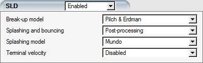
Select Pilch & Erdman to activate the break-up model. In
this case, a new governing equation is solved for the local diameter,  :
:

This equation models the evolution in time of the diameter , which becomes stable, after a characteristic time  . The source term is the speed at which the droplet reaches a
stable diameter
. The source term is the speed at which the droplet reaches a
stable diameter  . In this transport equation the diameter is imposed on the inflow
boundaries.
. In this transport equation the diameter is imposed on the inflow
boundaries.
The total break-up time depends on the break-up mechanism, or the local Weber number, according to the following relationships:

The dimensional time is obtained from  using the relative velocity between air and droplets,
 :
:

The maximum stable diameter  is estimated considering that the droplet break-up ceases when
their Weber number drops below 13:
is estimated considering that the droplet break-up ceases when
their Weber number drops below 13:

When the Pilch & Erdman model is enabled, the Droplets parameter - Particle type cannot be changed since the break-up mechanism is tied to the deformation phenomenon, for which a specific drag relation is required (See Droplet Deformation).
A droplet can reach a critical condition where its shape starts to deform due to the aerodynamic forces. These non-uniform pressure forces create surface waves on the droplet, while the surface tension tries to hold it together. Its shape begins to deviate from spherical to an oblate disk (not aligned with the flow). The drag coefficient of the droplet then begins to increase. At a critical moment, surface integrity can no longer be maintained and the droplet begins to break up.
Since deformation and break-up are strongly coupled, the following droplet deformation model is automatically activated if droplet break-up is selected (See Droplet Break-Up).
Below a Weber number of 13, the drag on a droplet is interpolated between that of a spherical drop and a disc (Schmel):

where:

and  is computed using an experimental correlation from Hsiang &
Faeth:
is computed using an experimental correlation from Hsiang &
Faeth:

This model modifies the droplet collection efficiency on the surface by predicting if all the impinging water bounces, or if a part of it splashes. In either case, no splashed or bounced droplets are re-introduced into the computational domain. The models used to predict the change in collection efficiency are described in Splashing and Bouncing by Body Force, Mundo Model and Honsek-Habashi Model.
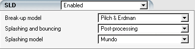
To activate this model, select the option in the Splashing and bouncing menu.
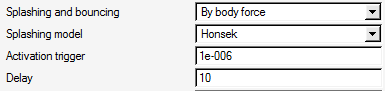
The model is a modification of the original droplet equations in which additional body forces are added in the vicinity of solid surfaces to simulate the effect of wall- droplet interactions on the droplet flow. It is activated by selecting the By body force option in the Splashing and bouncing menu:
The governing equations for the droplets become:


Where D, B and G are the forces due to drag, buoyancy and gravity per unit mass. The impact of splashing on the droplet momentum is modeled via a body force term applied on the elements connected to the impinging surface:

where  is the impact velocity of the primary droplets,
  is the velocity of the splashed droplets and
  is the collision time.
Since the body force model is based on the primary droplet impingement characteristics, it is activated only when the change of the primary droplet impingement reaches convergence. Convergence is detected when the change in total collection efficiency drops below the Activation trigger. The parameter Delay controls the number of iterations below the Activation trigger level before the activation of the body force model.
Note: Tetrahedral or pyramidal elements should not be placed on wall surfaces when the splashing-by-body-force model is activated.
The model is restricted to steady-state simulations.
To facilitate restarts after the body forces have been introduced in the simulation, an intermediate droplet solution file is saved when the change in total collection efficiency drops below the Activation trigger and the specified Delay is completed (See Solution Files with SLD).
The Mundo model is the default model for use with Splashing and bouncing by Post-processing. To select this model, set Splashing model to Mundo.

The Mundo model determines the probability of splashing or bouncing based on a Mundo parameter kM:

Where kC is the Cossali parameter defined by Weber and Ohnesorge number:

Splashing is said to occur when:

where  is an estimated non-dimensional roughness value set to
0.005.
is an estimated non-dimensional roughness value set to
0.005.
The secondary-to-primary droplet diameter ratio (ds/di) and the number of secondary particles (ns) is calculated as:


Subscripts s and i stand for secondary and primary particles respectively.
The secondary-to-primary droplet concentration can be defined as:

The Mundo model assumes that the collision between droplets and the wall is elastic, and the splashed droplet velocities are equal to the impingement velocities (see Referenced Within This Manual):


where subscripts n and t correspond to the normal and tangential orientations of the velocity vector.

The Honsek model is the default model for use with Splashing and bouncing by Body force. To select this model, set Splashing model to Honsek.

The Honsek-Habashi model determines the probability of splashing, bouncing or disintegration based on a threshold computed by Trujillo and Lee.

Splashing if the Cossali parameter  . The number of splashed particles are defined as:

The secondary to primary droplet concentration is calculated as:


The droplet diameter ratio, normal and tangential velocity ratio is calculated as:

Bouncing occurs if  and is characterized within a Weber number range:

The secondary to primary droplet parameters are calculated as:


To select this model, set Splashing model to Wright.

The Wright model determines the probability of splashing or bouncing based on corrections made to the Mundo parameter described in Mundo Model:

The Wright parameter  is defined from
  by considering impingement velocity angle with respect to the
surface normal:
by considering impingement velocity angle with respect to the
surface normal:

Splashing occurs if  . The secondary to primary droplet parameters are calculated
as:
. The secondary to primary droplet parameters are calculated
as:


In Body forces → , select in the Terminal velocity box to activate this option, otherwise, select . If this option is enabled, the magnitude and direction of the gravity vector must be specified.
Note: The gravity vector should be perpendicular to free stream velocity if level-flight conditions are being simulated.
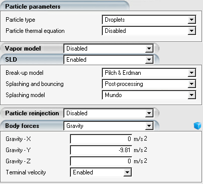
Due to their larger MVD, SLD droplets cannot be assumed to remain in static atmospheric suspension but rather they behave like rain drops falling with a terminal velocity. Hence, an additional vector component is introduced in the droplets initial approach velocity, resulting in an altered impingement trajectory.
Since the droplet velocity appears in both the drag coefficient and the droplet Reynolds number, there is a general difficulty in establishing correlations expressing a droplet's terminal velocity in terms of the corresponding Reynolds number. Hence, a dimensionless quantity known as the Galileo number may be defined as a function of physical properties of the gas and liquid phase in order to eliminate the unknown terminal velocity:

Khan & Richardson derive a comprehensive correlation expressing the Reynolds number as a function of the Galileo number:

Once the terminal Reynolds number is evaluated, the corresponding terminal velocity may be obtained from:

which is added to the inflow droplet velocity.
The gravity vector components must be set in order to enable the terminal velocity. Furthermore, the Galileo number is computed from reference properties that are constant over the computational domain, hence the use of terminal velocity with space or time-dependent boundary conditions has no relevance.