


To guarantee the correct simulation of ice accretion, the reference conditions must be identical to those of the airflow and droplet solutions.
These reference conditions are used to link the ICE3D calculation to its
corresponding air and droplet solution. Enter the reference characteristic length
 , freestream air velocity
  , freestream static air temperature
  and air static pressure
  . The values must be identical to those used for the airflow and
droplet calculations.
. The values must be identical to those used for the airflow and
droplet calculations.
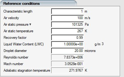
The reference pressure can also be computed from the altitude. To do so, click Air static pressure and select Altitude. ICE3D automatically computes the pressure based on the U.S. Standard Atmosphere (1976).
ICE3D also computes the reference air Reynolds and Mach numbers for verification purposes. These two non-dimensional numbers should be identical to those computed for the air solution.
The reference conditions are also used to link the ICE3D calculation to its
corresponding droplets solution. Enter the reference Liquid Water Content
LWC ( )
)  .
.
Important: The Air static temperature is used by ICE3D only to convert the heat fluxes from the airflow solver into convective heat transfer coefficients. It is NOT the temperature at which the icing simulation is performed. The icing simulation is conducted at the Icing air temperature, which most of the time is the same as the Air static temperature. These two temperatures, when used judiciously, permit the simulation of different icing conditions using a single air solution.
The Recovery factor
 is used to introduce the effect of the energy losses due to
friction when computing the total temperature from the static temperature and
the Mach number:
is used to introduce the effect of the energy losses due to
friction when computing the total temperature from the static temperature and
the Mach number:

 is set to unity by default, implying that the surface
temperature is the stagnation temperature computed from freestream conditions. A
recovery factor less than unity implies that:
is set to unity by default, implying that the surface
temperature is the stagnation temperature computed from freestream conditions. A
recovery factor less than unity implies that:
The heat fluxes from FENSAP are converted into convective heat transfer coefficients using the recovery reference temperature.
The convective heat transfer coefficient is multiplied by the recovery ice temperature in the energy balance equation.
Good judgement should be used when setting a value of recovery factor less than unity. An empirical formula to compute a value for the recovery factor on a flat plate is:

where  is the laminar Prandtl number. This formula yields
  for
for 
This section provides more information regarding two crucial parameters: the Icing air temperature and Ice density.
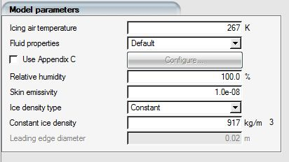
The Icing air temperature is the static temperature at which ice accretion is computed. It can be thought of as the temperature of the icing cloud. The surface recovery temperature, vapor pressure, and the droplet temperature will be based on the Air static temperature. ICE3D’s icing model allows the user to set the icing temperature different than the reference temperature used in the airflow simulation, to simulate different icing conditions using the same airflow solution. The airflow solution essentially provides the heat transfer coefficients, while the droplet and surface recovery temperature are computed with the Icing air temperature. The recovery temperature depends on the recovery factor (See The Recovery Factor).
Note that changing the Icing air temperature ignores the changes in Mach number, and large deviations from the reference temperature at which the airflow was calculated should be done with care. For quick workflows using a single airflow solution and studying a range of icing temperatures, obtaining this airflow solution at a temperature close to the center of the range is recommended.
Note: For internal flows and turbomachinery icing simulations, icing air temperature variation is not a recommended method to study different icing conditions. In such cases, even the reference temperature setting may not reflect the inlet air static temperature. Internal icing cases are best simulated using particle thermal equation, vapor transport, and adiabatic-wall air flow solutions with EID enabled.
Water and ice are the default media, and their thermodynamic characteristics are automatically supplied to ICE3D. To select another fluid/solid media combination or to select different properties for water and ice, select the Advanced option. This gives access to the fluid properties menu.
The relative humidity is expressed as a percentage value. For clouds, this value should be set to 100%. Otherwise, enter the relative humidity of the icing tunnel, as determined during the experiment. If a vapor solution is provided, this option is not required and will be greyed out. To facilitate the use of a wet bulb temperature setting to figure out the relative humidity for the icing air temperature, one can click on the button to the right of the Relative humidity % value box and enter the wet bulb temperature in Kelvins:
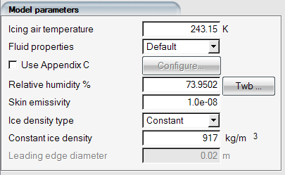
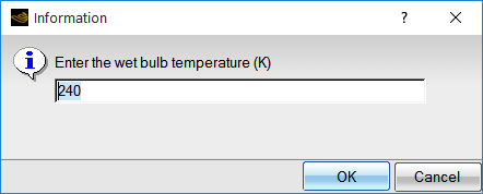
This function calculates the saturation vapor pressures at specified wet bulb temperature and icing air temperature, from the empirical formula found in D.M. Murphy and T. Koop, Review of the vapor pressure of ice and supercooled water for atmospheric applications, 2005, Quarterly Journal of the Royal Meteorological Society. The temperature range for which this function is valid is 123 – 332K.
The skin emissivity indicates whether radiation effects are taken into account by ICE3D (black body, or 1.0). If not, enter a low emissivity (1.e-8 for example).
Ice density can be set to:
A constant value (the default value for ice is 917 kg/m3). This option should be used to compare ICE3D results with other ice accretion results obtained with a fixed ice density.
Based on the Macklin formula:
 for 0.2 < RM < 170
where

 is the droplet diameter in microns,
  is the droplet impact velocity, in m/s and
  is the wall temperature from ICE3D, in degrees
Celsius.
is the wall temperature from ICE3D, in degrees
Celsius.Based on the Jones (glaze) formula:
 (in g/cm3)
The Impact Ice Density model is created by Ansys especially for swept wing icing simulations, inspired by the void density model in NASA’s LEWICE3D. It is meant to be used as part of multishot icing with remeshing workflow, to help generate realistic ice shapes with feathers and scallops. The studies for the AIAA Ice Prediction Workshops showed that this density model is essential in capturing accurate scallop formations that produce valid Maximum Combined Cross Sections (MCCS) both for glaze and rime conditions. It uses local droplet impact angle and freezing fraction to vary the density from 917 kg/m3 to 200 kg/m3. Perpendicular impact and low freezing fraction increase the density of ice which is closer to glaze ice, and the opposite reduces the density resembling feathery ice observed near the impingement limits of aircraft surfaces.
This model is currently included as beta, pending further calibration and validation.The model is controlled by three parameters: minimum rime ice density, maximum rime ice density, and blending coefficient:
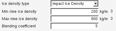
For glaze ice conditions, where the freezing fraction is closer to 0, the ice density will be closer to 917 kg/m3. In rime ice conditions, the ice density will be set between min and max rime ice density values entered in this panel. The maximum rime ice density value is used when the impact angle of droplets is 90° (perpendicular) to the surface. The minimum ice density value is set for an impact angle = 0° (tangent), which is a theoretical value that droplets will get close to at the impingement limits. The change from maximum to minimum rime ice density based on the impact angle value is done with a non-linear blending function, which is controlled by the blending coefficient. The range for this coefficient is 2 – 10. Higher blending coefficient values keep the ice density high for a wider range of impact angles. Currently the recommended value is 5, which is determined based on the swept wing ice accretion results from 1st and 2nd AIAA Ice Prediction Workshops. The variation of ice density with freezing fraction and impact angle is shown below
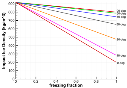
Impact ice density mode with blending coefficient = 5
See Appendix C for more information.
This section is required when running ICE3D in Conjugate Heat Transfer simulations (wet-air CHT3D) for complex geometries such as piccolo tube applications for aircraft anti-icing and jet engine nose cones, where the hot inner and cold outer airflow domains are connected but have distinct domain indices. In these cases the outside reference air conditions are ill-suited for the ICE3D evaporation model, which will also be required over the walls of the hot inner chamber.
To enable this option, click the Hot chamber reference evaporation conditions check box.
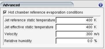
The Jet reference static temperature is the static temperature of the jet. The Jet effective static temperature is normally also the jet static temperature, but it can be varied to study the effect of different jet temperatures on the effectiveness of the IPS without recomputing the airflow solution. Velocity is the jet velocity and Relative humidity is the relative humidity of the hot air jet.