


Select the option in the Physical model menu to enable the FENSAP flow solver.
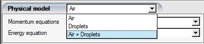
Additional physical models are and .
The grid file should be assigned before setting up the input parameters, since some of them, such as the boundary conditions, are grid-dependent.
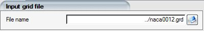
The grid file should be assigned using the grid icon in the run window, however it can also be reset in this panel. In this case, however, only grids in FENSAP format are allowed, FENSAP-ICE will not automatically verify the format of the grid file and prompt for conversion. The grid file is then read to detect the boundary conditions. Note that if the grid is replaced with a different one, it is imperative to review the configuration of the boundary conditions.
The flow field is modeled by partial differential equations for the conservation of mass, momentum and energy. The conservation of mass for a compressible flow, for example one where the density of the fluid is not a linear function of both pressure and velocity, can be written as:

where  is the density and
  is the velocity vector. The subscript
  refers to the air solution. This equation is also known as the
continuity equation.
refers to the air solution. This equation is also known as the
continuity equation.
For a Newtonian fluid, Newton second law of motion states that the total force acting on a fluid particle is equal to the time rate of change of its momentum. This can be written in 3D using a set of 3 non-linear equations, shown here in vector form:

which are known as the Navier-Stokes equations, where  is the stress tensor, or:


 is the static pressure and
  is the dynamic viscosity. The special case of inviscid fluid
flows, where the dynamic viscosity is set to zero, yields the Euler
equations.
is the dynamic viscosity. The special case of inviscid fluid
flows, where the dynamic viscosity is set to zero, yields the Euler
equations.
For a viscous laminar flow, the viscosity is defined empirically by Sutherland law:

where  refers to the static air temperature in Kelvin, and where the
subscript ∞ indicates reference values for air:
refers to the static air temperature in Kelvin, and where the
subscript ∞ indicates reference values for air:  = 288 K and
  = 17.9 10-6 Pa s.
This laminar viscosity is constant and is computed using the reference air static temperature of the Conditions panel of FENSAP-ICE.
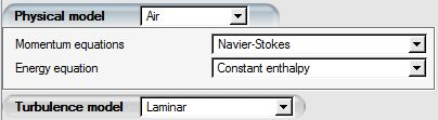
For viscous flows, select . For inviscid flows, select in the Physical model section.
The third physical principle concerns the conservation of energy and states that the total energy of the system must be conserved, or:

where  and
and  are the total internal energy and enthalpy, respectively,
 is the ratio of specific heats which equals 1.4 for air (perfect
gas), and κ is the thermal conductivity, computed in a similar way to the
laminar dynamic viscosity:
is the ratio of specific heats which equals 1.4 for air (perfect
gas), and κ is the thermal conductivity, computed in a similar way to the
laminar dynamic viscosity:

where refers to the static air temperature in
Kelvin, and where the C1 is equal to  .
.
The laminar dynamic viscosity is constant and is computed using the reference air static temperature of the Conditions panel of FENSAP-ICE.
To solve for the energy equation, select .
The set of eight flow equations with nine unknowns, expressed in a primitive
variable form ( ), describes the steady laminar (viscous, non-turbulent) flow. The
equation required to close the system is the equation of state for an ideal
gas:
), describes the steady laminar (viscous, non-turbulent) flow. The
equation required to close the system is the equation of state for an ideal
gas:

where  = 287.053763 KJ/kg is the Gas Constant for air. This equation can
be transformed into the algebraic constant stagnation enthalpy equation for
steady-state inviscid flows, shown below.
= 287.053763 KJ/kg is the Gas Constant for air. This equation can
be transformed into the algebraic constant stagnation enthalpy equation for
steady-state inviscid flows, shown below.
If the Ideal Gas option is selected (default), the properties of the fluid are defined using the reference static temperature and remain constant everywhere. If the Real Gas option is selected, the fluid properties are a function of the local static temperature and vary throughout the solution domain.
If the following assumptions are true:
The flow is adiabatic.
No heat is absorbed nor radiated from the volume.
No heat is conducted in the fluid.
The fluid is chemically inert.
No work is done on the fluid.
The potential energy of the fluid is constant.
Then the full energy equation in PDE form can be converted to an algebraic equation that implies that the stagnation enthalpy remains constant along streamlines:

To select this option, choose .
Note: This option reduces the computational effort, but can only be applied to flows that satisfy the conditions listed above.
By default, FENSAP solves the energy equation in non-conservative form, which results in robust convergence especially when the momentum and energy systems are uncoupled. It is also possible to solve this equation in Conservative Form, which increases heat flux accuracy for transonic flows. This is currently a beta feature, pending full integration with actuator disks and unsteady flows with mesh displacement (ALE). To have it visible in the energy equation options in the model panel, Show advanced / beta solver options in the → → General tab must be checked. This will bring the two additional options Full PDE – Conservative and Energy-only – Conservative in the Energy equation selection box.
A variety of turbulence models have been implemented in FENSAP. All models are based on the statistical approach to turbulence, for example all the variables are time-averaged and a steady flow is computed. The effect of turbulence is represented in the momentum equations via the eddy viscosity hypothesis. The turbulence models provide the spatial distribution of the eddy viscosity which is then used in the momentum equations.
To select this turbulence model, choose in the turbulence models section.
The turbulence model is a one-equation
model. It is based on the transport of a modified eddy viscosity  from which the effective eddy viscosity coefficient
 is computed.The modified eddy viscosity is related to the
effective eddy viscosity such that:
is computed.The modified eddy viscosity is related to the
effective eddy viscosity such that:

where  is obtained from the transport equation:

with

|

|

|
and d is the distance to the nearest wall.
The two functions  and
and  are defined as

|

|
where

and  is the laminar kinematic viscosity. The destruction term
is:
is the laminar kinematic viscosity. The destruction term
is:

where

|

|
The closure coefficients of the model are set as follows:
|
|
|
|
|


The following parameters are available for the Spalart-Allmaras model implementation in FENSAP:
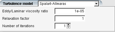
The eddy/laminar viscosity ratio is used to compute the initial turbulent viscosity coefficient when starting the calculation. For external flow calculations, and if the incoming flow is not turbulent, this parameter should be set to a low (but not zero) value, for example 10-5 (default). For internal flows, it should be increased to 1 or higher.
The eddy/laminar viscosity ratio is used for initialization as well as boundary condition at inlets, unless a turbulence profile is specifically provided.
The turbulence equations are solved separately from the Navier-Stokes equations. The Number of iterations is the number of turbulence iterations per Navier-Stokes iteration. The default value is 1. For difficult to converge problems with strong turbulent features, increasing this parameter to 3 can be tried before reducing the CFL for the whole system.
The Relaxation factor is used when updating the turbulence variables. For Spalart-Allmaras, a value of unity (default) is strongly recommended. A lower value can be used if the turbulence equation becomes unstable (erratic convergence) or the residuals and/or lift and drag coefficients oscillate in steady-state calculations.
The  turbulence model is based on the transport of the turbulent
kinetic energy
turbulence model is based on the transport of the turbulent
kinetic energy  , and the second transported scalar
  can be interpreted as a frequency because of its dimension
equivalent to 1/time.
can be interpreted as a frequency because of its dimension
equivalent to 1/time.
The transport equations are:


The default model coefficients are set as follows:


and the eddy viscosity is given by:

To select this turbulence model, choose Low-Reynolds K-omega in the list of turbulence models.
The eddy/laminar viscosity ratio is used to compute the initial turbulent viscosity coefficient when starting the calculation. For external flow calculations, and if the incoming flow is not turbulent, this parameter should be set to a low (but not zero) value, for example 1 (default value) or below. For internal flows, it should be increased to 50 to 100.
Turbulence intensity ( ) represents the level of turbulence and is usually shown in
percentage. It is defined as the ratio of the root-mean-square of velocity
fluctuations to the mean velocity magnitude. The default value of turbulence
intensity in FENSAP is 1%. For low-turbulence case, for example an incoming
external flow approaching an aircraft, the turbulence intensity can be well
below 1%. In this case,
) represents the level of turbulence and is usually shown in
percentage. It is defined as the ratio of the root-mean-square of velocity
fluctuations to the mean velocity magnitude. The default value of turbulence
intensity in FENSAP is 1%. For low-turbulence case, for example an incoming
external flow approaching an aircraft, the turbulence intensity can be well
below 1%. In this case,  = 0.08% is recommended. For internal flows, the turbulence
intensity is typically high, which may vary from 1% to 5% for medium-turbulence
cases and increase up to 20% for high-turbulence cases. The local turbulent
kinetic energy
= 0.08% is recommended. For internal flows, the turbulence
intensity is typically high, which may vary from 1% to 5% for medium-turbulence
cases and increase up to 20% for high-turbulence cases. The local turbulent
kinetic energy  is computed from
  :
:

The turbulence equations are solved separately from the Navier-Stokes equations. The number of iterations is the number of turbulence iterations per Navier-Stokes iteration. You should select a value between 1 (default) and 3 (difficult situations).
The relaxation factor is used in the update of the turbulence variables. For
the  model, a value of 1 (default) is recommended. However, a lower
value should be selected if the turbulence equations become unstable (erratic
convergence).
model, a value of 1 (default) is recommended. However, a lower
value should be selected if the turbulence equations become unstable (erratic
convergence).
The transport equations of Menter’s SST
 model are


where the blending function  is defined by

with

and  is the distance to the nearest wall.
  is equal to zero away from the surface (
 ), and switches over to one inside the boundary layer
().
), and switches over to one inside the boundary layer
().
The turbulent eddy viscosity is defined as follows:

where  is the invariant measure of the strain rate, for example,
 and
and  is a second blending function defined by

A production limiter is used in the SST model to prevent the build-up of turbulence in stagnation regions:

All constants are computed by a blend from the corresponding constants of the
 and the
  models via
  . The constants for this model are:
The following settings are provided for the k-ω SST model.
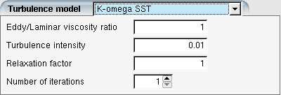
The eddy/laminar viscosity ratio is used to compute the initial turbulent viscosity coefficient when starting the calculation. The default value is set to 1 which represents a non-quiescent flow. For flows in free-stream using a far-field boundary, this value can be reduced to 1e-5.
The eddy/laminar viscosity ratio is used for initialization as well as the boundary condition at inlets, unless a turbulence profile is specifically provided.
Turbulence intensity is set to 1% (0.01) by default. For flows with a far-field, this value can be set to 0.0008.
The Relaxation factor is used when updating the turbulence variables. For , a value of unity (default) is strongly recommended. A lower value can be used if the turbulence equation becomes unstable (erratic convergence) or the residuals and/or lift and drag coefficients oscillate in steady-state calculations
The turbulence equations are solved separately from the Navier-Stokes equations. The Number of iterations is the number of turbulence iterations per Navier-Stokes iteration. The default value is 1. For difficult to converge problems with strong turbulent features, increasing this parameter to 3 can be tried before reducing the CFL for the whole system.
Note: If a simulation that converges well with the
diverges with kω-SST, it is
recommended to increase the Number of iterations of
turbulence to 3 to prevent divergence.
Select for a smooth wall, otherwise several sand-grain roughness options are available. All three turbulence models currently available in FENSAP-ICE can simulate constant and variable sand-grain roughness distributions.
If the Specified sand grain-roughness option is selected,
the Nikuradse equivalent sand-grain roughness height,
 (in meters) should be provided.
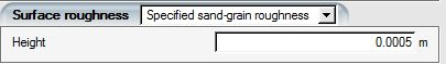
The roughness is set to a value of 0.5 mm by default when activated, but can be modified if required.
Tip: Although it is possible to specify arbitrary roughness values, past a certain limit (~ 5-10 mm for a wing) where the roughness height would trigger macroscopic flow separation effects, roughness should be simulated at the surface geometry and grid level, rather than through the turbulence model.
If is selected, the surface sand-grain roughness is computed with an empirical NASA correlation for icing.
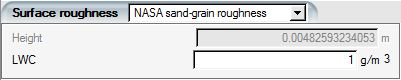
The sand-grain roughness value is computed from the product of the following coefficients:


where LWC is the liquid water content, and
 . The corresponding value of sand-grain roughness is obtained
from the formula:
. The corresponding value of sand-grain roughness is obtained
from the formula:

and is shown by the graphical interface in the Height field.
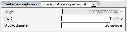
If the is selected, the empirical correlation for the surface sand-grain roughness is computed with the Shin and Bond formula, which modifies the NASA correlation with the following factor:

where  is the droplet mean diameter, in microns. The corresponding
value of sand-grain roughness is obtained from:
is the droplet mean diameter, in microns. The corresponding
value of sand-grain roughness is obtained from:

and is displayed by the graphical interface in the Height box.
If the option is selected, the sand-grain roughness will be read from a node-based input file (See The Sand-Grain Roughness Distribution File (roughness.dat)). The input file must be named roughness.dat and copied in the FENSAP run directory.
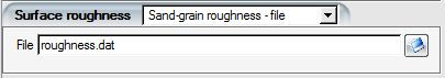
ICE3D writes a roughness.dat file that can be used for multishot ice accretion.
If the option is selected, individual sand-grain roughness values can be assigned to any wall surfaces listed in the Boundaries panel.

When this option is selected, an additional sand-grain roughness value assignment box appears for each wall family listed in the Boundaries conditions panel. The roughness.dat file will then be created automatically by FENSAP-ICE.
The FENSAP-ICE system provides a very unique and powerful means of accounting for the roughness of the ice shapes through the beading model. Strictly speaking, the roughness due to the water beading process is computed by the ICE3D module based on local conditions on the contaminated surface (See Beading).
In multishot ice accretion simulations, the roughness data can be transferred to the flow solver to compute the appropriate shear stresses and heat fluxes. The roughness due to the freezing of the beads is both spatially- and temporally-dependent, hence it is useful only in the context of a fully unsteady calculation, or in the multishot approach, which is a more cost-effective quasi-steady approximation of the fully unsteady simulation.
The multishot configuration procedure is described in Multishot Run Creation and Basic Configuration. With this approach, when the beading model is selected in the ICE3D configuration, FENSAP-ICE will automatically perform all the necessary steps to link the roughness data with the flow solver.
Two transition mechanisms are available in FENSAP with the turbulence model. The transition is enabled in the Transition section of the Model panel.
If the turbulence model is selected, transition can be imposed. If no transition is selected, the boundary layer will be fully turbulent.
With the Fixed transition option, transition is imposed in the turbulence model through tripping functions and a special boundary index set in the grid file (See FENSAP-ICE File Formats) at the fixed transition location. At least one wall boundary facet in the grid must be assigned to this index. This index (2,000 to 2,999) is specified with the Transition BC index. The Fixed transition model injects a small amount of turbulence in the boundary layer to trigger transition.
The tripping intensity, which is the coefficient “ct1” in Spalart’s model, is set by default to 1. To compute the transition length, the orientation of the airfoil chord should be given, either along the X-, Y- or Z-axis.
Note: The laminar-turbulent transition can occur ahead of the transition BC, if the latter is placed too far downstream.
With the Free transition option, transition from laminar to turbulent is automatically set by FENSAP based on adverse pressure gradients.
For the SST  turbulence model, a one-equation local correlation-based
intermittency transition model is available. It integrates experimental correlations
into standard convection-diffusion transport equation using local variables. The
transport equation of intermittency
turbulence model, a one-equation local correlation-based
intermittency transition model is available. It integrates experimental correlations
into standard convection-diffusion transport equation using local variables. The
transport equation of intermittency  is
is

In the production term, the function  determines the length of transition. The formulation of the
function
determines the length of transition. The formulation of the
function  , which is used to trigger the intermittency production, contains
the ratio of the local vorticity Reynolds number
, which is used to trigger the intermittency production, contains
the ratio of the local vorticity Reynolds number  to the critical Reynolds number
  :
:


The absolute value of stain rate  and vorticity
  are defined as

The critical Reynolds number is computed algebraically using local variables:

in which


In the formulation of 
 , where
  is the velocity vector and
  is the wall-normal vector. The model constants are:

The coupling between the transition model and the SST  turbulence model is accomplished by modifying the production
 and destruction term
  of turbulent kinetic energy equation:


Moreover, an additional production term  has been introduced into the
  -equation to ensure proper generation of
  at transition points for arbitrary low
  level. It is designed to turn itself off when the transition
process is completed and the boundary layer has reached the fully turbulent state.
The expression for the additional source term reads as
level. It is designed to turn itself off when the transition
process is completed and the boundary layer has reached the fully turbulent state.
The expression for the additional source term reads as


where the constants are

The blending function  in SST that is responsible to switching between the
  and
and  models is reformulated as follows:

Two different types of body force can be applied during simulations.
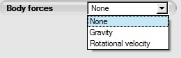
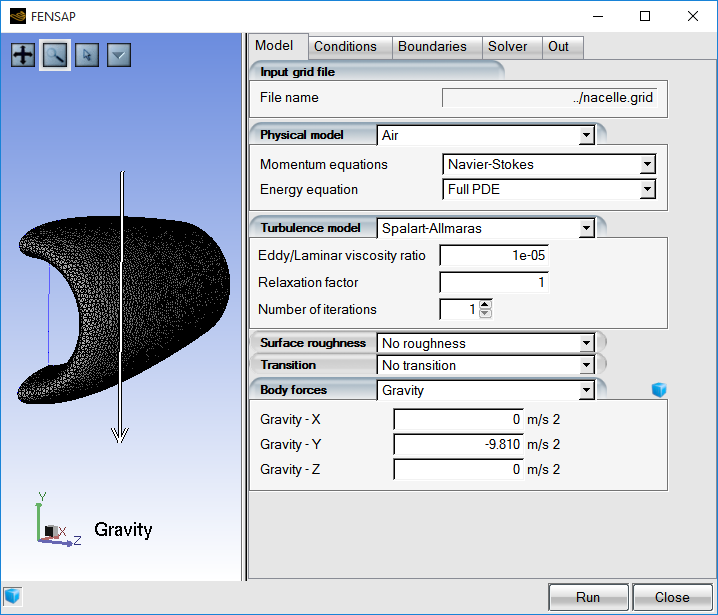
Select None to neglect gravity (typical of most CFD applications). For convection-driven problems, the force of gravity can be included by adding the following source term to the right-hand side of the Navier-Stokes equations:

To do so, select Gravity in the list of body forces.
Enter the components of the gravity vector in the body force window. Click the
display icon ![]() to display the gravity vector in the graphical window as
shown in the following figure.
to display the gravity vector in the graphical window as
shown in the following figure.
Click the display icon ![]() again to remove the gravity vector from the graphical
window.
again to remove the gravity vector from the graphical
window.
Important: When gravity is activated, the pressure applied at the exits will be automatically calculated using the barometric formula to account for the pressure gradient that naturally occurs in the stratified atmosphere and the static pressure set at the far field or exit boundary. In external air flow simulations with large far fields, failure to do so would result in significant inaccuracies in the boundaries and possibly cause divergence.
Finally, the gravity vector should be adjusted with respect to the angle of attack specification.
For CFD calculations in a steadily rotating frame of reference (for example rotors), select the Rotation speed option in the Body forces section.
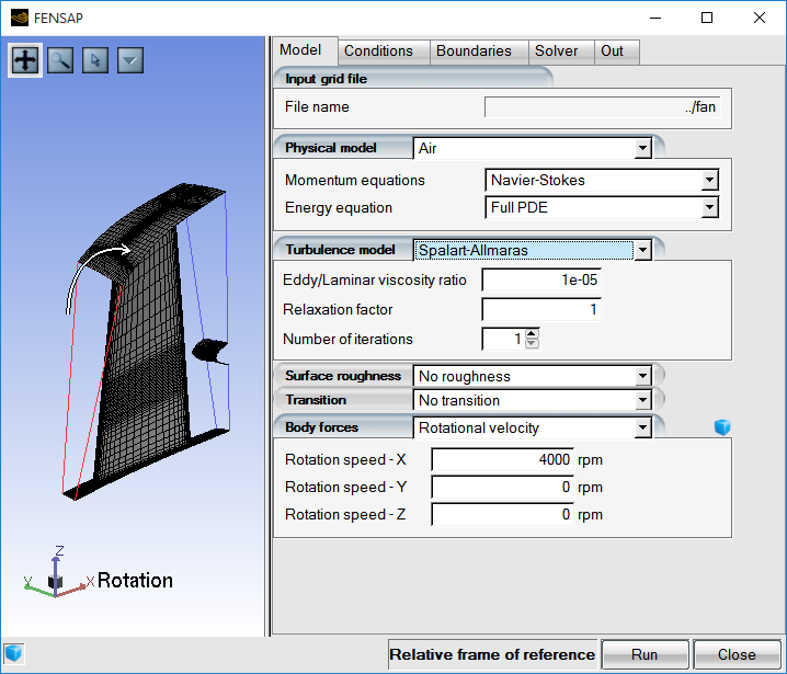
The three components of the rotation speed Ω should then be entered in the Body force window.
The center of rotation is located at the origin (0,0,0). Source terms are added to the momentum equations to introduce the Coriolis and centrifugal forces acting on the fluid in the relative frame:

If at least one of the three components is non-zero, a reminder that the frame of reference has been switched to relative will appear at the bottom of the FENSAP window.

Note: The default frame of reference is absolute. If a rotational velocity is specified, the frame of reference becomes relative, for example, the entire grid is rotating. The velocity vectors are written in absolute components in the solution file. If the solution is used as a restart, the presence of the rotational velocity components in the header of the FENSAP solution file will automatically trigger conversion to relative components. When visualizing the solution with Viewmerical, both the absolute and relative velocities will be available for display.
Tip: In some cases to accelerate convergence of steady-state flows it is beneficial to initialize the domain inside rotating components with the rotation rate of the component. More details can be found in Multi-Domain Initialization.