The next figure shows the heat and mass transfer phenomena modeled when solving for ice accretion and runback. On each solid surface, the contamination caused the by impinging droplets is modeled as thin liquid film. The film may run back, forced by the shear stresses created by the airflow, by a centrifugal force, or by gravity. The height of the liquid film is to be determined at all grid points on the solid surfaces. Based on the surface thermodynamic conditions, part of the film may freeze (ice accretion), evaporate or sublimate.

The velocity of the water film is a function of the coordinates x=(x1,x2) on the surface and y (normal) to the surface. The problem is simplified by introducing a linear profile for the film velocity (x,y), normal to the wall, with zero velocity imposed at the wall:

where , the air shear stress, is the main driving forces for the film. This assumption is justified by the thin film thickness, seldom greater than 10 μm in icing or anti-icing simulations. By averaging the film velocity across the film thickness, a mean velocity can be derived as follows:

ICE3D solves a system of two partial differential equations on all solid surfaces. The first equation expresses mass conservation:

where the three terms on the right hand side correspond, respectively, to the mass transfer by water droplet impingement (source for the film), by evaporation and by ice accretion (sinks for the film).

The second partial differential equation expresses conservation of energy:

where transfer generated by the impinging supercooled water droplets, by evaporation and by ice accretion. The last three terms are the radiative, convective and 1D conductive heat fluxes that could be supplied by an anti-icing heater device.

The coefficients are physical properties of water and ice that are adjustable in the user interface.

The reference conditions are airflow and droplets parameters specified by you. They should match the values used in air flow and droplet runs.

The local wall shear stress and the convective heat flux should be supplied by the flow solver.

DROP3D provides local values of the collection efficiency β, droplet energy and droplet impact velocity .

The evaporative mass flux is recovered from the convective heat transfer coefficient, using a parametric model.

is the anti-icing heat flux obtained from C3D for wet air calculations.

Three unknowns remain to be computed: the film thickness , the equilibrium temperature at the air/water film/ice/wall interface and the instantaneous mass accumulation of ice .

Compatibility relations are needed to close the system of equations. Based on physical observations, one way to write them is as follows:

These inequalities ensure that the model predicts no liquid water when the equilibrium temperature is below the freezing point (0˚C), and that no ice forms if there is film that is above 0˚C.

From the above equations and variables, some of the most common icing parameters such as the freezing fraction and the impact angle can be computed and are exposed inside ICE3D’s solution file.

The freezing fraction is defined as the ratio between the ice accretion rate and the incoming water flux within a control volume. The incoming flux is composed of impingement and film flux arriving from neighboring grid nodes. Freezing fraction is a value between 0 and 1, reaching 1 for rime ice nodes while remaining close to 0 on nodes that are ice-free.

The impact angle is defined as the angle in degrees between the particle impingement direction and the local surface tangent plane on the grid node. The impact angle changes from 90 to 0 degrees as one moves away from the stagnation line towards the impingement limits.

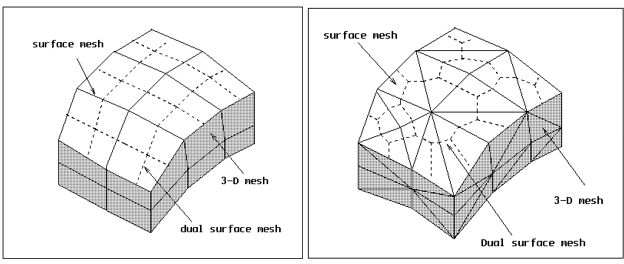
The governing equations are formulated for curvilinear two-dimensional surfaces embedded in three-dimensional geometries. The boundaries of the three-dimensional mesh at the air-structure/ice shape interface are denoted as the 3D surface mesh. From the surface mesh, a 3D dual surface mesh is automatically obtained by connecting the mid-edges of the cells to cells' centroids. The discrete equations are then solved with the finite volume method on this dual mesh.