


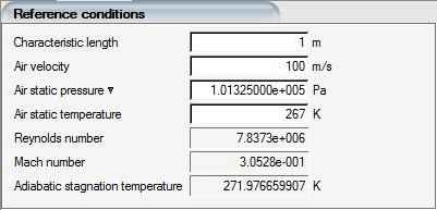
Since the set of discrete particle equations is in non-dimensional form, a set of suitable reference conditions are required.
The air and particle equations could be solved simultaneously (as in a two-phase flow). However, since the density of a water droplet is 1,000 times greater than the density of air and the water fraction is dilute, the equations are solved in a segregated manner. The airflow is solved first, followed by the particle equations. In other words, the effect of the air on the particle is considered, but not the reverse.
It is important, however, to ensure that the reference conditions for the particle calculation, for example the reference Reynolds and Mach numbers, remain the same as in the associated airflow calculation.
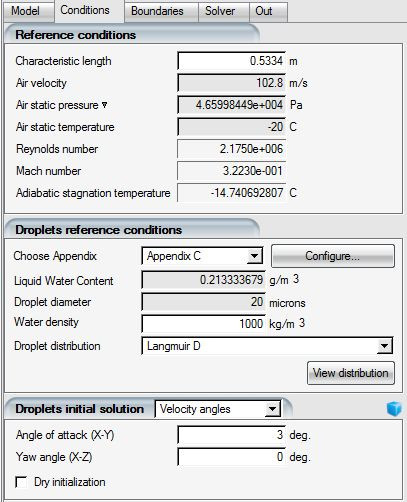
Note: When carrying out icing simulations with FENSAP-ICE, it is highly recommended that the reference conditions represent the icing cloud conditions and the true air speed (TAS) of the aircraft or test article. In case of helicopter rotor analysis, the blade tip speed is the ideal choice for reference velocity. The reference conditions are used to non-dimensionalize the model equations and the collection efficiency. Certain numerical aspects in DROP3D that are used to improve stability and convergence in the shadow zones will be affected by these settings. Characteristic length should have no impact on the solution other than changing the scale of the residual plots.
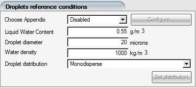
The main physical parameters describing the droplets are:
The Liquid Water Content (LWC): the density of water droplets in the air.
The Droplet diameter,  : spherical droplets are assumed to be of a single, uniform size,
usually equal to the median volume diameter (MVD) of the sample size distribution.
The Droplet diameter is in microns.
: spherical droplets are assumed to be of a single, uniform size,
usually equal to the median volume diameter (MVD) of the sample size distribution.
The Droplet diameter is in microns.
The Water density,  : generally set to 1,000 kg/m3 for
water.
: generally set to 1,000 kg/m3 for
water.
The Droplet distribution: Built-in or user-defined.
Droplet Distributions
Several built-in droplet size distributions can be selected in the Droplet distribution pull-down menu of the Droplets reference conditions section of the Conditions panel:
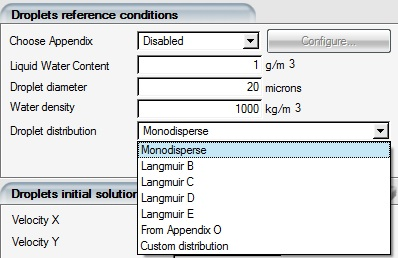
Monodisperse indicates a calculation performed for a single diameter, specified in the Droplet diameter.
Langmuir B to Langmuir E distributions can be simulated by computing the droplet concentration and speed for each individual diameter of the discrete distribution, which are subsequently automatically weight- averaged at the end of the simulation. The various Langmuir diameter distributions and their corresponding weights are pre-defined in FENSAP-ICE.
Custom distribution can also be selected (for example, in order to solve the same droplets distribution found in an icing tunnel).
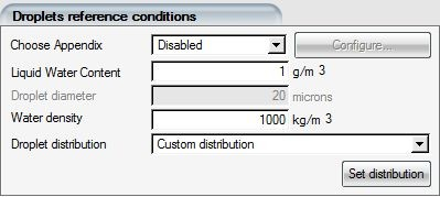
Click Set distribution to enter the droplet diameters and weights of the distribution. A window will then open to permit the definition the parameters.
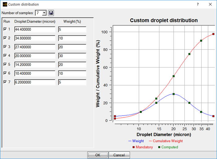
Important: Cumulative droplet diameter values must be entered from largest to smallest size.
Enter the Number of samples and define, for each of them, the Droplet Diameter (micron) and Weight (%) as percentage of LWC (the sum of this column should always be 100%). This distribution is simulated by computing the droplets concentration and speed for each diameter, and by applying the proper mass weighted averaging (%) to the individual droplets solutions. The graph shows the Weight (blue) and Cumulative Weight (red) curves of the distribution.
Particle diameter averaging is done based on the cube of the diameter:

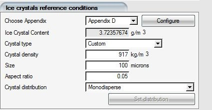
The ice crystals reference conditions require setting the Freestream crystal content, analogous to the Liquid water content, and the selection of a Crystal type and its Size.
Several predefined crystal types can be selected:
Hexagonal plate:
Predefined aspect ratio, only size can be configured.
Crystal-flat branches:
Predefined aspect ratio, only size can be configured.
Dendritic crystal:
Predefined aspect ratio, only size can be configured.
Solid thick plate:
Predefined aspect ratio, only size can be configured.
Custom:
Both size and aspect ratio can be configured.
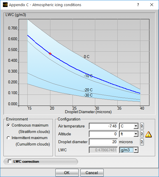
Appendix C contains three graphs per cloud environment type, which are built into FENSAP-ICE. The first graph from Appendix C can be viewed by selecting the Appendix C option in the Choose Appendix drop-down menu in the Droplets reference conditions section.
Clicking the button opens the configuration environment, which shows graphically the extent of the envelope covered by Appendix C.
The first graph relates to OAT (Outside Air Temperature), LWC and MVD. Since OAT is usually fixed in the airflow calculation, once the droplets size is selected FENSAP-ICE calculates the corresponding LWC. FENSAP-ICE displays both the isothermal curve in blue on the graph as well as the selected condition with a red cross symbol.
The original graphs from Appendix C can also be displayed by clicking
 on the right in the
Air temperature, Altitude and
Droplet diameter boxes in the
Configuration section shown in the following figure.
on the right in the
Air temperature, Altitude and
Droplet diameter boxes in the
Configuration section shown in the following figure.
The second graph of Appendix C relates pressure altitude to OAT. It can be viewed by pressing the question mark button (?) in the Altitude row. FENSAP-ICE will issue a warning if the chosen combination of altitude and temperature is outside the envelope of Appendix C.
The third graph from Appendix C relates LWC to the cloud extent. It can be viewed by pressing the question mark button (?) at the right of the scroll-down menu in the LWC correction section. The two icing cloud extent types, CM for Continuous Maximum and IM for Intermittent Maximum, have standard cloud extents of 33 and 5 nautical miles, respectively. Appendix C specifies that if the cloud extent considered differs from these values, the LWC must be corrected to maintain condition severity. A shorter cloud extent, therefore, leads to a higher LWC and conversely for longer horizontal extents.
Two environments are available: Continuous maximum, designed to represent stratiform clouds and Intermittent maximum for cumuliform clouds.
Click the LWC correction check box to display the LWC correction. If you are considering a component or system in forward flight, then the cloud extent is related to exposure time and true airspeed. Therefore, if exposure time is specified, FENSAP-ICE will calculate the equivalent cloud extent from the true airspeed and correct the LWC to reflect the change in severity. The other option is for FENSAP-ICE to calculate the exposure time required to traverse a cloud of standard extent.
Note: Air temperature, Altitude or Droplet diameter values outside the envelope of Appendix C will be displayed as red numerals.
To avoid conflicts with the reference conditions of the airflow solution when running the ice accretion simulation with ICE3D, it is not possible to override the Air static pressure and Air static temperature values set in the Reference conditions section. It is possible to edit the Altitude and Air temperature values to explore the envelope, but the new values will not be saved if they override the reference conditions. You should always make sure that the Reference conditions sections of the FENSAP, DROP3D and ICE3D configurations are identical.
Several drop diameter distributions can be selected with the Droplet distribution pull-down menu in the Droplets reference conditions section. The following figure shows the Langmuir D distribution.
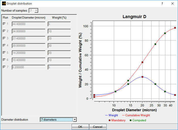
The droplet diameters and weights of the distribution are shown in the three columns on the left of the graph. The two curves show the weight distribution (blue) and cumulative weight distribution (red) as functions of the droplet diameter.
Two options are available in the pull-down menu at the bottom of the window:
7 diameters
4 diameters, enriched
If the 7 diameters option is selected, all diameters will be computed. If the 4 diameters, enriched option is selected, only four of the diameters will be computed and the remainder will be interpolated using Reduced Order Modeling.
Note: Reduced Order Modeling will reduce the execution time, however you must ensure that the technique is acceptable for their own needs. The legend below the graph indicates which diameters are computed and which diameters are interpolated.
Tip: You can edit the distribution by selecting Custom distribution in the Droplets reference conditions panel.
Appendix O is the proposed FAA aircraft certification regulation describing the Supercooled Large Droplets (SLD) icing conditions that may occur in and/or below the stratiform clouds defined in Appendix C of the FAA 14 CFR Part 25 certification guidelines. The FAA SLD environment is divided into two categories: the Freezing Drizzle (FZDZ) and the Freezing Rain (FZRA). The spectrums of droplet distributions of each category is further subdivided into two distribution subcategories: MVD < 40 μm and MVD > 40 μm, where the 40 μm reference value is the Maximum Effective (drop) Diameter (MED) of Appendix C icing conditions for Continuous Maximum stratiform clouds.
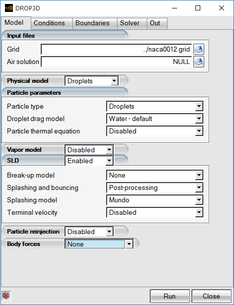
Enable the SLD option in the Model panel to gain access to the Appendix O functionalities. Three SLD related options will be revealed:
Break-up model
Splashing and bouncing
Terminal velocity
For all SLD simulations, a Splashing and bouncing model should be enabled. The Post-processing option is recommended.
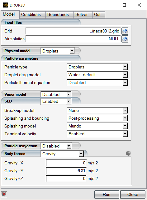
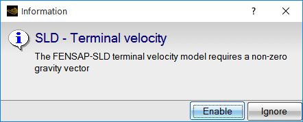
For FZRA conditions, the Break-up model should be set to Pilch & Erdman, and Terminal velocity should be Enabled. FZRA conditions include very large droplet sizes that are more sensitive to breakup phenomena and gravity. When Terminal velocity is Enabled, the appropriate direction of the Gravity vector must be defined in the Model panel. If not already set, FENSAP-ICE will prompt to enable Terminal velocity when the FZRA environment is selected.
FZDZ conditions do not include such large droplet sizes, they are not significantly affected by breakup and gravity. Therefore, these settings do not need to be enabled. Splashing and bouncing alone should be enough to characterize this environment.
Select to set the Terminal Velocity to a non-zero gravity vector.
The two environments and their parameters are set in the Droplet reference conditions section of the Conditions panel.
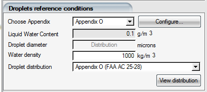
To access the Appendix O conditions, set Choose Appendix to . A message will appear asking you to select the Appendix O distribution. For now, select Appendix O (FAA AC 25-28). This is explained further in Choosing the SLD Droplet Distribution.
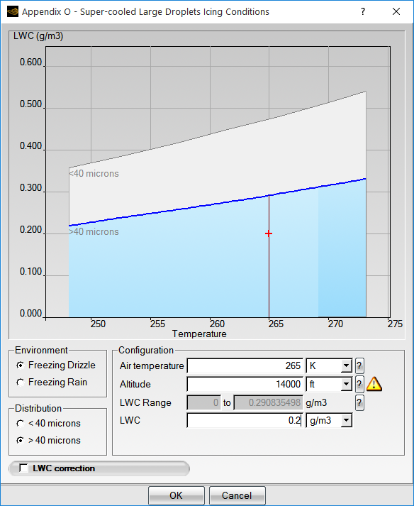
Click the button to open the Super-cooled Large Droplets Icing Conditions configuration window. The selected icing condition will be displayed in the active envelope as a red cross mark.
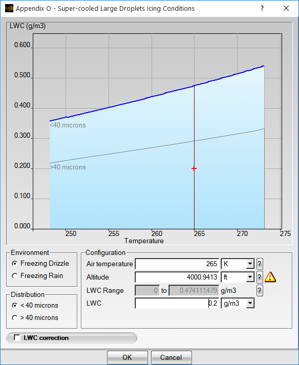
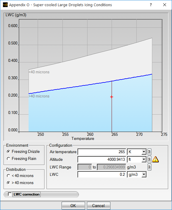
Select the desired Environment by clicking either the Freezing Drizzle or Freezing Rain button, and select the desired Distribution by clicking either the or button. If Terminal velocity and other required options are not already activated in the Model panel, DROP3D will issue warnings and prompt for their activation when clicking either of these buttons.
Note: The maximum liquid water content of the MVD > 40 μm distribution is smaller than for the MVD <40 μm droplet distribution.
Tip: The value of LWC can be edited in this panel and will override the value set in the Reference conditions.
Important: It is not possible to override the Air static pressure and Air static temperature values set in the Reference conditions section. This is done intentionally to avoid conflicts with the reference conditions of the FENSAP solution. It is possible to edit the Altitude and Air temperature values to visually explore the envelope in the window, but the new values will not be saved if they override the reference conditions. Always make sure that the values set in the Reference conditions sections of the FENSAP, DROP3D and ICE3D configurations are identical.
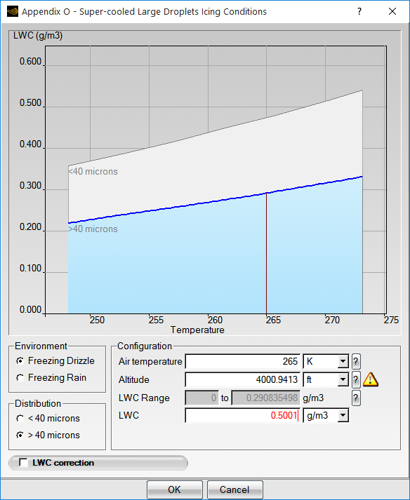
If the chosen values are outside the range of validity of the selected environment and its distribution sub-category, the value out of range will be displayed in red.
When the altitude exceeds 12,000 ft, temperature limits are activated and only the lighter part of the envelope is accessible. Temperature values that exceed the limit will be shown in red.
The original graphs from Appendix O can be consulted by clicking the question
mark ( ) buttons on the right of the configuration values.
Just as in Appendix C, the LWC can be corrected for either total time in the icing cloud or for cloud extent. Click the LWC correction check box to activate this option.
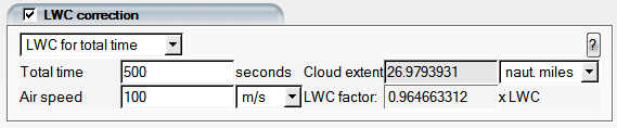
Select either the total time or the cloud extent with the pull-down menu and modify the relevant fields. The corrected value will be displayed as a blue cross on the graph.
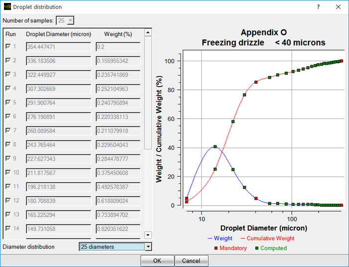
When Choose Appendix is set to Appendix O, a warning message appears prompting you to select a Droplet distribution.
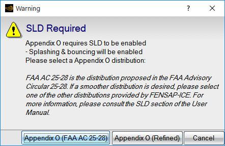
Select Appendix O (FAA AC 25-28) to set the Droplet distribution to the 10 diameter built-in distributions that were provided in Tables 1 and 2 of the FAA Advisory Circular AC 25-28 published October 27th, 2014.
Click the button to display the droplet distribution, as shown in the following figure.
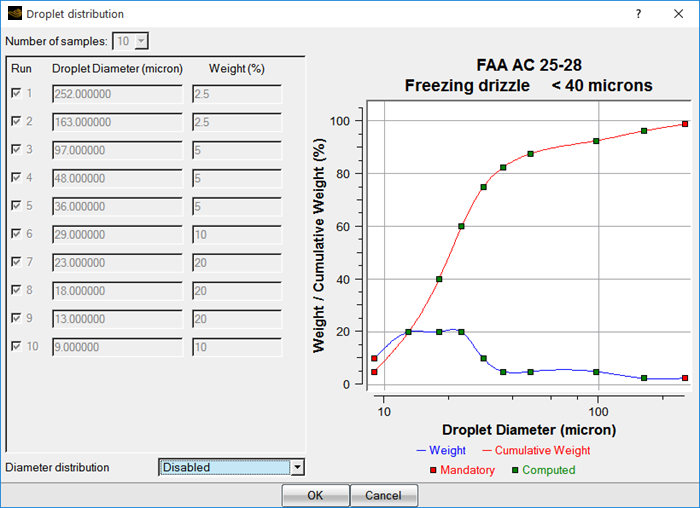
The title of the graph identifies the specific distribution that has been selected in the configuration window. The values of the weights for each droplet diameter are displayed in a table on the left, and the weight distribution (blue curve) and the cumulative weight distribution (red curve) are shown as functions of droplet diameter in the graph on the right.
Notice that the menu options for Diameter distribution are disabled at the bottom of the window. This is because, currently, there is only one diameter distribution provided for each environment in the FAA AC 25-28.
It should be noted that the FAA Advisory Circular AC 25-28 states:
" Applications of drop size distributions require a bin tabulation of the proportion of mass (liquid water content) to drop diameter. Mass proportions for the bins were selected to provide a reasonable resolution of the upper range of the distributions. The shaded columns (a) and (b) in the tables contain values typically used as input to ice accretion computer codes. For some simulation techniques, different methods of segregating the bins may be appropriate. "
The document suggests that the use of different distributions of droplet sizes and weights may be appropriate for some simulation techniques. Because of large jumps between simulated droplet sizes, the 10 diameter FAA AC 25-28 distribution may not produce a smooth representation of droplet impingement on wetted surfaces for many applications. In this instance, it may be useful to select one of the alternative distributions described below.
Alternative 1:
Select Appendix O (Refined) to access the alternative diameter distributions available in DROP3D. These distributions use a different diameter segregation method to provide a more refined definition of the Appendix O SLD environments.
Click the button to display the droplet distribution, as shown in the following figure.
Again, the values of the weights for each droplet diameter are displayed in a table on the left, and the weight distribution (blue curve) and the cumulative weight distribution (red curve) are shown as functions of droplet diameter in the graph on the right. If a distribution with enrichment (via ROM) has been selected, a legend is provided below the graph to indicate which diameters are computed and which diameters are interpolated.
There are now four options for Diameter distribution available in the pull-down menu at the bottom of the window:
25 diameters
10 diameters, enriched
25 diameters, enriched
97 diameters
These built-in distributions were constructed by using a 97 diameter representation to discretize the cumulative weight distribution curves provided in Appendix O to CFR Title 14 Part 25.1420. The computation of all 97 droplet diameters can become a resource intensive task, hence additional options are offered that take advantage of enrichment via Reduced Order Modelling (ROM). In this manner, you can select the one that best suits the available computational resources without paying a heavy penalty in accuracy.
If the 25 diameters option is selected, the SLD environments are represented using a smaller set of 25 points. The table to the left of the cumulative distribution curve shows the droplet diameters and their corresponding weights.
If the 10 diameters, enriched option is selected, only 10 of the 97 diameters will be computed and the remaining 87 diameters will be interpolated using ROM.
If the 25 diameters, enriched option is selected, 25 of the 97 diameters will be computed and the remaining 72 diameters will be interpolated using ROM.
If the 97 diameters option is selected, the full 97 diameter distribution will be computed. This is the most accurate but computationally expensive option.
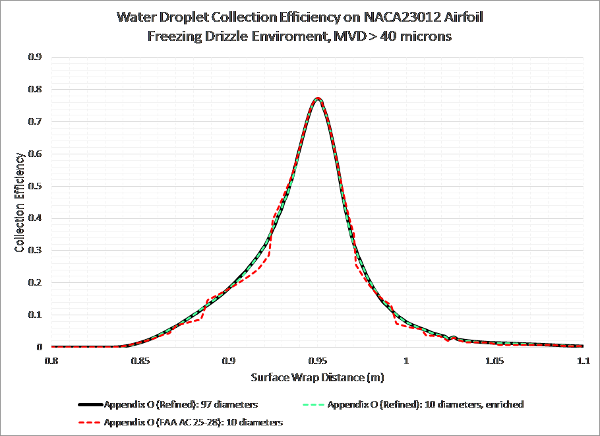
Note: The following curve shows the results of collection efficiency on a NACA23012 airfoil. The Freezing Drizzle environment, MVD > 40μm was simulated using three distributions:
Appendix O (Refined): 10 diameters, enriched
Appendix O (Refined): 97 diameters
Appendix O (FAA AC 25-28): 10 diameters.
Of the three simulated distributions, the Appendix O (Refined): 97 diameters provides the smoothest representation of the droplet environment, thanks to the relatively small changes between each simulated diameter, and it therefore produces a smooth collection efficiency curve. In this case, the Appendix O (Refined): 10 diameters, enriched also provides a smooth collection efficiency curve. The enrichment by Reduced Order Modelling (ROM) contributes significantly to the smoothness of the curve. However, the Appendix O (FAA AC 25-28): 10 diameters distribution produces a discontinuous collection efficiency. The large change in diameters between droplets contributes to these discontinuities. Therefore, in this case, it may be most appropriate to use the Appendix O (Refined): 10 diameters, enriched distribution as it provides a good level of smoothness while also offering a reduction in computational cost.
Alternative 2:
Finally, the Custom distribution option can be selected to enable the definition of user-defined custom droplet distributions. The droplet diameters specified in the Custom distribution must be listed in decreasing order. However once you select the Custom distribution option, DROP3D will immediately switch out of Appendix O, since DROP3D does not support custom distributions within the Appendix O environment.
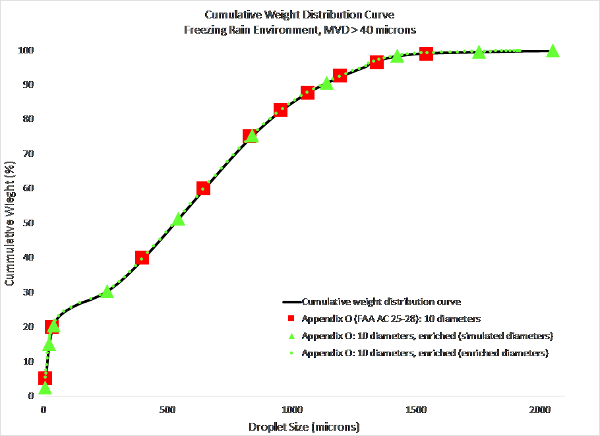
Note: The droplet sizes and weights in the Appendix O (FAA AC 25-28) and Appendix O (Refined) droplet distributions are different, because different discretization methods were used to create them. Both distributions describe the same SLD environments. The distributions are compared in the following figure. The black curve is the cumulative weight distribution that represents the Freezing Rain Environment, MVD > 40 microns, as outlined in the Appendix O regulations. The large red squares represent the droplet sizes and weights tabulated in the FAA AC 25-28 document, accessible in DROP3D by selecting Appendix O (FAA AC 25-28): . The large green triangles and small green dots represent the simulated and enriched droplet sizes and weights accessible in DROP3D by selecting : , enriched. Notice that both sets of points all lie on the same curve, however their positions are different. The FENSAP-ICE distributions are heavily weighted in the upper range of droplet diameters, where splashing and bouncing phenomena are more dominant.
Note: Reduced Order Modeling dramatically reduces execution time, however you must ensure that the technique is acceptable for your needs.
Splashing and bouncing effects tend to cause discontinuities in the individual collection efficiency curves of the larger droplets, therefore a larger number of droplet sizes may be required to produce smooth cumulative collection efficiency distributions.
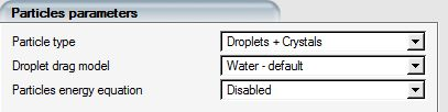
Appendix D is the proposed FAA aircraft certification regulation concerning Ice Crystals (IC) conditions associated with convective storms. In order to access the Appendix D configuration window, the Particle type in the Model panel should be set to Crystals or Droplets + Crystals.
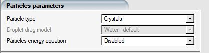
If only ice crystals are desired, select the Crystals option in the pull-down menu of the Particle parameters section.
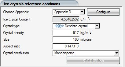
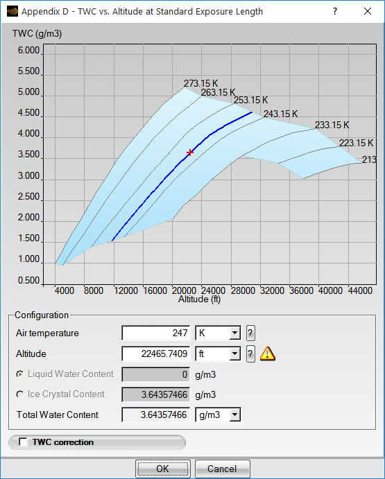
In the Ice crystals reference conditions section of the Conditions panel, set Choose Appendix to Appendix D and click the button to open the configuration window.
The configuration window gives access to the Air temperature and Altitude settings, from which the total water content is determined.
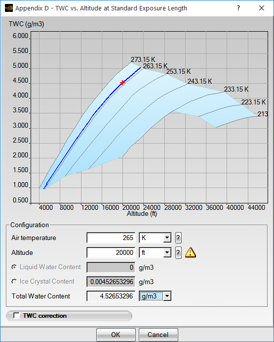
The selected conditions will appear in the envelope of Appendix D as a red cross. Select either the Liquid Water Content or the Ice Crystal Content to establish the ratio of the two particle types.
Important: It is not possible to override the Air static pressure and Air static temperature values set in the Reference conditions section, to avoid conflicts with the reference conditions of the FENSAP solution. It is possible to change the Altitude and Air temperature values in order to explore the envelope, however the values will not be saved. You should always make sure that the Reference conditions sections of the FENSAP, DROP3D and ICE3D configurations are identical.
Values outside the envelope of Appendix D will be shown in red.
If ice accretion calculations based on ice crystals are desired, a mixture of droplets and ice crystals should be selected. The physical reason for this choice is that crystals need a thin film of water in order to stick to a surface.
Choose the Droplets + Crystals option in the pull-down menu of the Particle parameters section.
In this case the reference conditions for both the droplets and the crystals must be set. Go to the Conditions panel and set the desired values in the Droplet reference conditions. When droplets plus crystals mixtures are used, the value of the Liquid Water Content is usually low, usually in the range from 0.1 to 1 gm/m3.
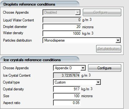
In the Ice crystals reference conditions panel, select Appendix D from the pull-down menu. Click Configure to display the configuration window.
Note: The value of the ICC (Ice Crystal Content) is automatically set by FENSAP-ICE. The graph displays TWC (Total Water Content) as a function of Altitude and Temperature.
Total Water Content is defined as:

The Total Water Content value can be corrected for time in the icing cloud or extent of the icing cloud by clicking the TWC correction check box. The TWC correction panel is similar to that of Appendix O.
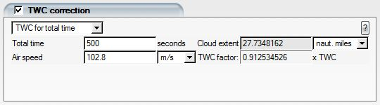
Select either the total time or the cloud extent with the pull-down menu and modify the relevant fields. The corrected value is displayed as a blue cross on the graph.
The Eulerian particle flow calculation is an iterative process like air flow calculation and requires initial conditions to be specified. There are several initial solution options to choose from.
Velocity Components
By default, the Liquid Water Content is initialized throughout the computational domain to its reference value.
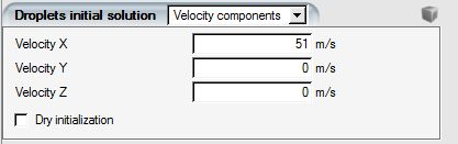
If the option is selected, the three components of the droplet velocity (Velocity X, Velocity Y and Velocity Z) are imposed as an initial guess throughout the computational domain.
Note: If the input grid file is in cylindrical coordinates, the velocity components
should be given as  (m/s),
  (rad/s) and
  (m/s).
Velocity Angles
If is selected, the three components of the initial droplet velocity vectors are computed from the two angles (See Velocity Angles and the norm of the reference velocity vector (See Reference Conditions).
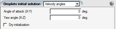
Note: The angle of attack is the angle of the velocity vector in the X-Y plane. The yaw angle is the angle of the velocity vector in the X-Z plane. Both angles are in degrees.
For difficult cases which have strong recirculation zones, the Liquid Water Content can be set to zero throughout the domain, except at the inflow boundaries, by checking the Dry initialization box.
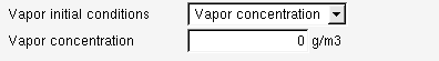
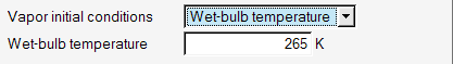
Vapor Initialization
Vapor field can be initialized with either vapor concentration, or relative humidity, or wet-bulb temperature. Relative humidity ranges from 0 to 100%. It is defined as the ratio of the partial vapor pressure to the saturation vapor pressure. When relative humidity is set as the initialization method, the local air temperature will be taken as reference on each grid node to calculate the corresponding vapor pressure and concentration. With wet-bulb temperature setting, the vapor pressure in the domain will be uniform and equal to 100% RH at that temperature, while its concentration will still depend on local air temperature using the partial pressure and partial density relationship with the gas constant for water vapor.
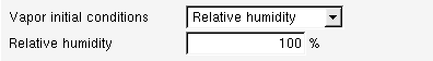
Note: Be careful when using RH option to initialize the vapor solution. The vapor concentration will be based on the local air temperature saturation pressure. High temperature regions like engine exhausts will start with equally high vapor concentrations which may not be the best solution strategy. In flows with hot exhausts, using vapor concentration for initialization may be a better option compared to using RH.
Dry Initialization
By default, DROP3D initializes the entire solution field using the reference Liquid Water Content or Ice Crystal Content value. In internal flows this may not be ideal since some regions may not receive any droplets and it may take a greater number of iterations to dissipate the non-zero water content values in these locations. For external flows, droplets that initially become trapped in strong recirculation zones may take a long time to clear out. In certain situations such issues can give rise to solution instabilities. Dry initialization is recommended in general, especially if there are strong recirculation zones in the airflow.
Input Profile
DROP3D can impose an inlet droplet velocity profile from a timebc.dat file. Select Input profile in the Droplet initial solution menu.
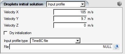
If the Input profile type is set to TimeBC
file, use  to open the browse window and select the appropriate timebc.dat
file. timebc.dat files are files generated by FENSAP/DROP3D
and ICE3D to exchange node-based information among modules. See The timebc.dat file for more information on the format of these
files.
to open the browse window and select the appropriate timebc.dat
file. timebc.dat files are files generated by FENSAP/DROP3D
and ICE3D to exchange node-based information among modules. See The timebc.dat file for more information on the format of these
files.
Input Rotational Profile
In turbomachinery each stage has its own grid, coupled to the preceding and following rows at their interfaces through the pitch averaging procedure. The airflow solution process is based on a recursive sweep through the stages with bi-directional data exchange from one stage to its neighbors at the interfaces.
Select the Rotational DROP3D solution option in the Input profile type box.
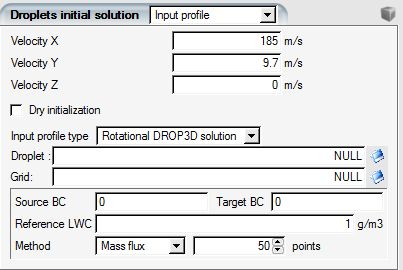
The rotation speed is set in the Body forces section of the Model panel. Stationary stages have a rotation speed of 0 rpm. Source BC refers to the index of the outflow boundary of the preceding row, while Target BC refers to the boundary index of the inflow boundary of the following row. The figure above shows the configuration for a non-rotating stage with inlet BC 1000 and outlet BC 3000. The Reference LWC is the liquid water content of the first component in the series, required to correctly compute the water impact efficiency since as the droplets proceed through the rows some water mass is lost in each row due to impingement on the blades, the hub and shroud.
Two methods are available for the boundary conditions: Mass flux is a mass-weighted pitch averaging, while Averaging refers to simple pitch averaging. The averaging is computed using N points equidistant from the rotational axis across the passage. Mass flux averaging is selected by default.
If ice crystals are enabled, the input solution file name for ice crystals is also required. The corresponding reference Ice Crystal Content value must also be set in the panel.
Dry Zone Initialization
In some regions, such as enclosures which are connected to the main flow but where the water droplets are not expected to penetrate, for example the inner cavity of an engine nose cone, it may be desirable to initialize and maintain dry conditions (zero LWC). To enable this option, in the Domains panel, select the domain that is expected to remain dry and set its Initial conditions to Dry zone:
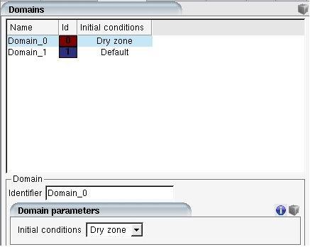
Note: The grid file must contain more than one domain for this option to be accessible. See The Domains Table for more information on domain IDs.
The Dry initialization condition is different than Dry zone, which does not allow the droplet solution to change, maintaining zero water content at all times and excluding this zone from the calculation of the average residuals.
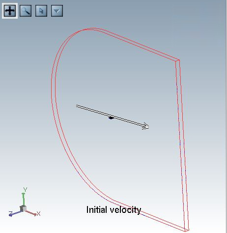
Click the display icon ![]() to display the Initial velocity vector in the graphical
window. Click the icon again to remove the velocity vector from the graphical
window.
to display the Initial velocity vector in the graphical
window. Click the icon again to remove the velocity vector from the graphical
window.
If Solution restart is selected, the droplets field is initialized with a previous droplet solution read from a file.
Starting with version 24R2, vapor solution fields are also saved in droplet and crystal files to simplify post processing. When restarting from a droplet file, if the vapor fields are in the file they will be used as restart data. If not, the vapor initial conditions parameters will be used instead to initialize vapor fields.
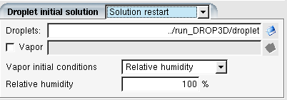
Click the browse icon to open the file browser and select the solution file to be used for restarting the calculation.
Note: The restart file must have the same number of nodes as the current grid.