


The following topics are included in this section:
You can review your results in the Graphics window using objects such as contours, vectors, pathlines, particle tracks and XY plots. You can also create surfaces for further exploring the results.
These different post-processing tools are generally distributed into the following groups: Surfaces, Graphics objects, Plots and Reports. For quick access to commonly used commands, a context-sensitive menu is available when right-clicking within the Graphics window.
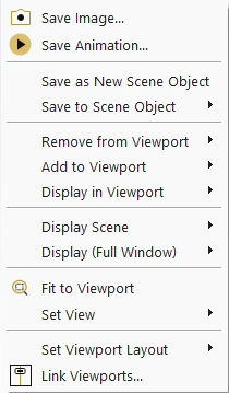
: Opens the Save Picture dialog box allowing you to save an image file of the object in the Graphics window.
: Opens the Save Animation dialog box allowing you to save an animation file.
Note: This setting is active only for transient datasets.
: Saves the Graphics window content as an object under Scenes.
: Saves the Graphics window content to an existing Scene object.
: Adds the selected Graphics object to the viewport.
: Displays the selected Graphics object within the viewport.
: Removes the selected Graphics object from the viewport.
: Displays the selected Scene object in the viewport.
: Displays your model to take maximum advantage of the Graphics window's width and height.
: Adjusts the overall size of your model to take maximum advantage of the viewport's width and height.
: Contains a drop-down of views, allowing you to display the model from the direction of the vector equidistant to all three axes, as well as in different axes orientations.
: Allows you to select from a collection of viewport arrangements.
: Synchronizes the display of the selected viewports.
You can create different types of surfaces to visualize your results, including points, lines, rakes, planes, iso-surfaces, and iso-clips.
Note: To ensure updated surface definitions (for example, if you change the location of a line) are properly shown when included in a Scene or other Graphics object, display the surface before re-displaying the containing object.
Refer to the following sections for more details:
You may be interested in displaying results at a single point in the domain. For example, you may want to monitor the value of some variable or function at a particular location. To do this, you must first create a Point surface, which consists of a single point. When you display node-value data on a point surface, the value displayed is a linear average of the neighboring node values. If you display cell-value data, the value at the cell in which the point lies is displayed.
![]() Results → Surfaces
Results → Surfaces
![]() New
→ Point...
New
→ Point...
To create a point surface, use the Figure 36.4: Properties of a Point Surface dialog.
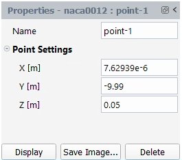
The following options are available when creating a point surface:
Name
(Optional) Provide a name for the point surface if you do not want to use the default name.
Point Settings
Specify the location of the point by entering the X, Y, Z coordinates.
Once you have set your properties:
Click at the bottom of the point properties to display the points in the Graphics window.
Click to open the Save Picture dialog box and proceed to save an image file of the object in the Graphics window.
Click at the bottom of the point properties to delete a point.
A line is simply a line that extends up to and includes the specified endpoints. Data points will be located where the line intersects the faces of the cell, and consequently may not be equally spaced.
![]() Results → Surfaces
Results → Surfaces
![]() New
→ Line...
New
→ Line...
To create a line surface, use the Figure 36.5: Properties of a Line Surface.
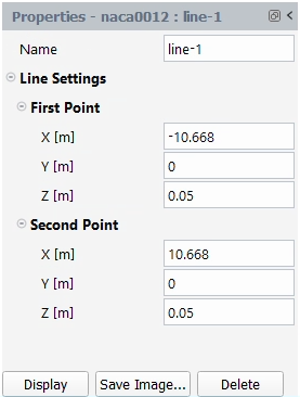
The following options are available when creating a line surface:
Name
(Optional) Provide a name for the line surface if you do not want to use the default name.
First Point
Specify the location of the first point by entering the X, Y, Z coordinates.
Second Point
Specify the location of the second point by entering the X, Y, Z coordinates.
Once you have set your properties:
Click at the bottom of the line properties to display the line in the Graphics window.
Click to open the Save Picture dialog box and proceed to save an image file of the object in the Graphics window.
Click at the bottom of the line properties to delete a line.
A rake consists of a specified number of points equally spaced between two specified endpoints.
![]() Results → Surfaces
Results → Surfaces
![]() New
→ Rake...
New
→ Rake...
To create a rake surface, use the Figure 36.6: Properties of a Rake Surface.
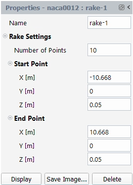
The following options are available when creating a rake surface:
Name
(Optional) Provide a name for the rake surface if you do not want to use the default name.
Number of Points
Set the number of points to include in the rake surface.
Start Point
Specify the location of the start point by entering the X, Y, Z coordinates.
End Point
Specify the location of the end point by entering the X, Y, Z coordinates.
Once you have set your properties:
Click at the bottom of the rake properties to display the rakes in the Graphics window.
Click to open the Save Picture dialog box and proceed to save an image file of the object in the Graphics window.
Click at the bottom of the rake properties to delete a rake.
To display flow-field data on a specific plane in the domain, you will use a plane surface. You can create surfaces that cut through the solution domain along arbitrary planes.
Note: Planes that are co-planar with a domain boundary may not appear as expected due to the clipping process for ensuring smooth boundaries.
![]() Results → Surfaces
Results → Surfaces
![]() New
→ Plane...
New
→ Plane...
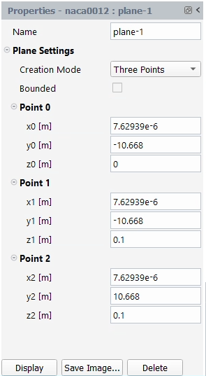
To create a plane surface, use the Figure 36.7: Properties of a Plane Surface.
There are three types of plane surfaces that you can create (via the Creation Mode):
XY, ZX, YZ Plane
The plane is created in the , , or directions, bounded by the extents of the domain. You can move the plane to the desired location in the domain using the plane tool. For example, if you are using the YZ Plane method, you can drag the plane in the (+) or (-) X direction.
The plane orientation is determined by selecting a point and specifying a direction normal to that point. The extents of the plane are the edges of the domain. You have the option to control the orientation of the plane using the plane tool or you can compute the normal from a surface.
The plane orientation and extents are bounded by three points that you can select. You also have the option to manipulate the points and orientation of the plane directly in the Graphics window using the plane tool.
Point and Normal
Name
(Optional) Provide a name for the plane.
Point 0 and Normal
Drag the plane tool to the desired location, as shown in The Plane Tool for the Point and Normal Method in the Fluent User's Guide.
Alternatively, you can specify Point 0 and the Normal by providing the coordinates of each.
Three Points
Name
(Optional) Provide a name for the plane.
Important: The surface name that you enter must begin with an alphabetical letter. If the name of the surface begins with any other character or number, Fluent Post-Analysis rejects the entry.
Toggle to have your plane bounded by the extents of the domain.
Point 0, Point 1 and Point 2
Drag the plane tool to the desired location, as shown in The Plane Tool for the Three Points Method in the Fluent User's Guide.
Alternatively, you can specify Point 0, Point 1, and Point 2 by providing the coordinates.
XY, ZX, YZ Plane
Name
(Optional) Provide a name for the plane.
Important: The surface name that you enter must begin with an alphabetical letter. If the name of the surface begins with any other character or number, Fluent Post-Analysis rejects the entry.
Z, Y, X [m]
Specify the plane direction.
Once you have set your properties:
Click at the bottom of the plane properties to display the planes in the Graphics window.
Click to open the Save Picture dialog box and proceed to save an image file of the object in the Graphics window.
Click at the bottom of the plane properties to delete a plane.
If you want to display results on cells that have a constant value for a specified variable, you will need to create an iso-surface of that variable. Generating an iso-surface based on x-, y-, orz- coordinate, for example, will give you an x, y, or z cross-section of your domain. Generating an iso-surface based on pressure will enable you to display data for another variable on a surface of constant pressure. You can create an iso-surface from an existing surface or from the entire domain. Furthermore, you can restrict any iso-surface to a specified cell zone.
Important: You cannot create an iso-surface until you have initialized the solution, performed calculations, or read a data file.
![]() Results → Surfaces
Results → Surfaces
![]() New
→ Iso-Surface...
New
→ Iso-Surface...
To create an iso-surface, use the Figure 36.8: Properties of an Iso-Surface.
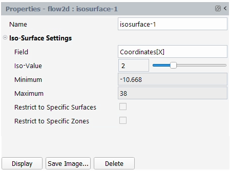
The following options are available when creating an iso-surface:
Name
(Optional) Provide a name for the iso-surface.
Important: The surface name that you enter must begin with an alphabetical letter. If the name of the surface begins with any other character or number, Fluent Post-Analysis rejects the entry.
Field
Click to open the Field dialog box and specify the field you want to view.
Click to confirm your selected field and close the dialog box.
Iso-Value
Enter the iso-values. You can enter multiple iso-values into the field separated by spaces.
Minimum
Specify the minimum range value of the selected field.
Maximum
Specify the maximum range value of the selected field.
Toggle to restrict the iso-surface to a particular surface. When toggled on, a Surfaces option will appear allowing you to select multiple surfaces.
Toggle to restrict the iso-surface to a particular zone. When toggled on, a Zones option will appear allowing you to select multiple zones.
Once you have set your properties:
Click at the bottom of the iso-surface properties to display the iso-surface in the Graphics window.
Click to open the Save Picture dialog box and proceed to save an image file of the object in the Graphics window.
Click at the bottom of the iso-surface properties to delete an iso-surface.
Instead of creating plane surfaces one at a time as described above, you have the option to create multiple plane surfaces at once using the Figure 36.10: Create Multiple Planes Dialog Box.
Iso-clip surfaces are clipped surface that consist of those points on the selected surface where the scalar field values are within the specified range.
![]() Results → Surfaces
Results → Surfaces
![]() New
→ Iso-Clip...
New
→ Iso-Clip...
To create an iso-clip surface, use the Figure 36.9: Properties of an Iso-Clip Surface.
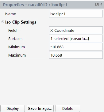
The following options are available when creating an iso-clip surface:
Name
(Optional) Provide a name for the iso-clip surface.
Field
Click to open the Field dialog box and specify the field you want to view.
Click to confirm your selected field and close the dialog box.
Surfaces
Select a surface to apply to the iso-clip.
Minimum
Specify the minimum range value of the selected field.
Maximum
Specify the maximum range value of the selected field.
Once you have set your properties:
Click at the bottom of the iso-clip properties to display the iso-clip in the Graphics window.
Click to open the Save Picture dialog box and proceed to save an image file of the object in the Graphics window.
Click at the bottom of the iso-clip properties to delete an iso-clip.
Instead of creating plane surfaces one at a time as described above, you have the option to create multiple plane surfaces at once using the Figure 36.10: Create Multiple Planes Dialog Box.
![]() Results → Surfaces
Results → Surfaces
![]() Create Multiple Planes...
Create Multiple Planes...
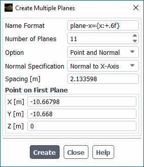
The following options are available when creating multiple planes:
Name Format
(Optional) Provide a format for naming the plane surfaces.
Number of Planes
Specify how many planes will be created.
Option
Select the method for how you want to create the planes.
Point and Normal
Similarly to the process described earlier in this section, you must provide a point and the direction normal to that point to define the first plane.
Normal Specification
Specify the direction normal (perpendicular) to the plane.
Spacing [m]
Specify how far apart the planes are from each other.
Point on First Plane
Provide the coordinate for the location of the first plane.
First and Last Point
You define the coordinates for the first and last point, which determines the orientation of the planes. The spacing is determined by how many planes you specify in the Number of Planes field.
Spacing [m]
Specify how far apart the planes are from each other.
Point on First Plane
Provide the coordinate for the location of the first plane.
Point on Last Plane
Provide the coordinate for the location of the last plane.
Click to create the new plane surfaces.
The new plane surfaces created using the Create Multiple Planes dialog box are added to the Outline View tree under the Surfaces branch and are now eligible for editing individually.
Note: Once created, the multiple planes cannot be edited as a group.
Once you have set your properties:
Click at the bottom of the plane properties to display the planes in the Graphics window.
Click to open the Save Picture dialog box and proceed to save an image file of the object in the Graphics window.
Click at the bottom of the plane properties to delete a plane.
Instead of iso-surfaces one at a time as described above, you have the option to create multiple iso-surfaces at once using the Figure 36.11: Create Multiple Iso-Surfaces Dialog Box.
![]() Results → Surfaces
Results → Surfaces
![]() Create Multiple Iso-Surfaces...
Create Multiple Iso-Surfaces...
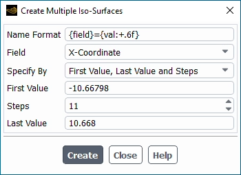
The following options are available when creating multiple iso-surfaces:
Name Format
(Optional) Provide a format for naming the iso-surfaces.
Field
Select the field that you want to use for creating the iso-surfaces.
Specify By
Specify the method you want to use for creating iso-surfaces.
First Value, Last Value and Steps
Using this method you must specify the First Value for the quantity that you selected in the Field drop-down list, specify how many iso-surfaces you want created by entering the number of Steps, and provide the final value for the selected quantity in the Last Value field.
First Value, Last Value and Increment
Using this method you must specify the First Value for the quantity that you selected in the Field drop-down list, specify the size of the increments between the first and last value, which determines the number of iso-surfaces to be created, and provide the final value for the selected quantity in the Last Value field.
First Value, Increment and Steps
Using this method you must specify the First Value for the quantity that you selected in the Field drop-down list, specify the size of the increments from the first value, and provide the total number of steps in the Steps field, which determines the total number of iso-surfaces to be created.
Last Value, Decrement and Steps
Using this method you must specify the size of the decrement (negative increment) in the Decrement field, which will go backwards from the Last Value, provide the total number of steps in the Steps field, which determines the total number of iso-surfaces, and provide the final value for the selected quantity in the Last Value field.
Click to create the new iso-surfaces.
The new iso-surfaces created using the Create Multiple Iso-Surfaces dialog box are added to the Outline View tree under the Surfaces branch and are now eligible for editing individually. Once created, the multiple iso-surfaces cannot be edited as a group.
Once you have set your properties:
Click at the bottom of the iso-surface properties to display the iso-surfaces in the Graphics window.
Click to open the Save Picture dialog box and proceed to save an image file of the object in the Graphics window.
Click at the bottom of the iso-surface properties to delete an iso-surface.
Post-processing Graphics objects are available for visualizing the results of your simulation. You can display the mesh, contours, vectors, pathlines, and scenes. Scenes allow you to combine multiple Graphics objects within a single Graphics window.
Note: Only field variables that are appropriate and compatible for the specific workspace simulations are available in the Field dialog box.
Once you have created your Graphics objects and/or made changes to their properties, you can:
Click to take maximum advantage of the Graphics window's width and height.
Click to display the selected Graphics object within the viewport.
Click to display the results between two identical or different datasets using a specific viewport layout.
Click to open the Save Picture dialog box and proceed to save an image file of the object in the Graphics window.
Click to open the Save Animation dialog box and save an animation file.
Click to delete the object in the Graphics window.
Select multiple items in the Outline View to perform a bulk function (such as using to remove multiple surfaces at a time).
The available graphics objects are described in greater detail in the following sections:
The Line Integral Convolution algorithm allows you to integrate a vector over a part surface. It can be used to provide a uniform visualization of the flow of a vector over a surface.
Line integral convolution can be drawn as part of contour objects or mesh objects in which faces are displayed. To draw LIC, choose Contours or Mesh Outline. The settings used for drawing the LIC including the velocity field can be specified under LIC Settings in the Outline View.
![]() Results → Graphics
→ LIC SettingsNew...
Results → Graphics
→ LIC SettingsNew...
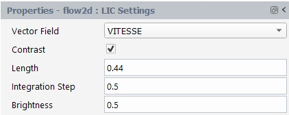
The following options are available when creating lic settings:
Vector Field
Choose an existing vector variable to display on the surface.
Contrast
Select to do a pass of image contrast enhancement.
Length
Specify a maximum length of 20 pixel units in the positive and negative directions. Length is a scaling factor of this 20 pixels. Range is 0 to 1.
Integration Step
Specify the step size in pixel units for each integration step. Range is 0 to 1.
Brightness
Specify the surface brightness. Range is 0 to 1.
Mesh plots allow you to visualize and inspect the mesh.
To create a mesh plot, right-click Meshes in the Outline View tree and select New....
![]() Results → Graphics
→ Meshes
Results → Graphics
→ Meshes![]() New...
New...
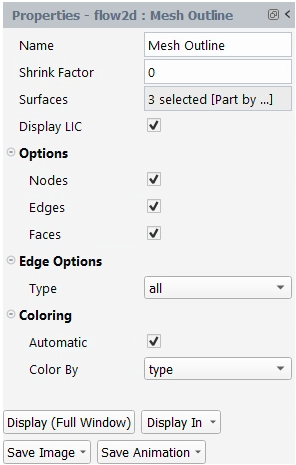
The following options are available when creating mesh plots:
Name
(Optional) Enter a name for the mesh object.
Shrink Factor
(Optional) Enter a shrink factor.
Surfaces
Select the surfaces where you want the mesh displayed by selecting the desired surfaces in the Surfaces dialog box and clicking .
Display LIC
Select to display the line integral convolution.
Options
Nodes
Displays the mesh nodes.
Edges
Displays the mesh edges.
Faces
Displays the mesh faces.
Edge Options
Set which edges you want displayed:
Type
all
Displays all of the edges.
feature
Displays only the features and outline of the mesh.
outline
Displays only the outline of the mesh.
Coloring
Specify how you want the mesh to be colored:
Automatic
Automatically colors the mesh based on the selection in the Color by drop-down list (either by type, id or material).
Color By (Automatic disabled)
Allows you to set a color for the mesh faces and edges.
Color Faces By
Specify a color to apply to faces.
Color Edges By
Specify a color to apply to edges.
Color Nodes By
Specify a color to apply to nodes.
Contour plots are a valuable post-processing tool that allow you to use color to represent the values of the specified field variable on the selected surfaces.
To create a contour plot, right-click Contours in the Outline View tree and select New....
![]() Results → Graphics
→ Contours
Results → Graphics
→ Contours![]() New...
New...
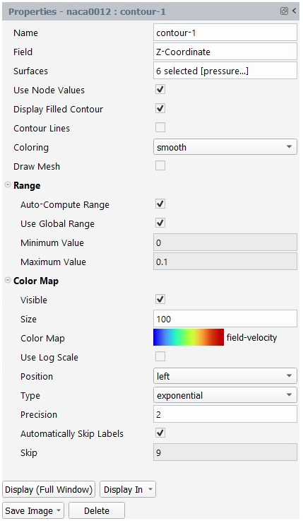
The following options are available when creating contour plots:
Name
(Optional) Enter a name for the contour object.
Field
Specify the field variable you want to display.
Surfaces
Select the surfaces where you want the contours displayed by selecting the desired surfaces in the Surfaces dialog box and clicking .
Use Node Values
Displays the values at the nodes.
Display Filled Contour
Displays contours that are fully colored.
Display LIC
Displays the line integral convolution.
Contour Lines
Displays lines on the plot corresponding to the gradations in the colormap.
Coloring
Specify whether contours are banded or smooth.
Draw Mesh
Displays whichever mesh you select in the Overlayed Mesh drop-down list, which includes the outline and any defined mesh objects.
Range
Set the range for the contour plot:
Auto-Compute Range
Automatically calculates the range for the contour colormap. When disabled, it allows you to clip the range to a specified Minimum and Maximum.
Use Global Range
Confirms that you are using the automatically computed range. However, if you do not want to use this range, you must disable Auto-Compute Range.
Minimum Value and Maximum Value
Allows you to set the range for the contour plot values. These fields only apply when you disable Auto-Compute Range.
Color Map
Set the color map fields:
Visible
Toggle to have the color key displayed along with the contour display.
Size
Determines the size of the colormap.
Color Map
Specifies the colors to be used in the colormap display.
Use Log Scale
Uses a logarithmic scale.
Position
Determines where the colormap is located in the Graphics window.
Type
Set whether the colormap follows a general, float, or exponential scale.
Precision
Set the number of significant digits for the colormap.
Automatically Skip Labels
Select to skip a certain number of labels (or show all) in the contour color map.
Skip
Set a spacing on the colormap scale.
Volume rendering displays all 3D elements at once, drawing each element semi-transparently according to the value of a variable using user-selected x, y, and z dimensions to control the number of elements passed up to the client.
To create a volumetric rendering, right-click Volume Rendering in the Outline View tree and select New....
![]() Results → Graphics
→ Volume
Rendering
Results → Graphics
→ Volume
Rendering![]() New...
New...
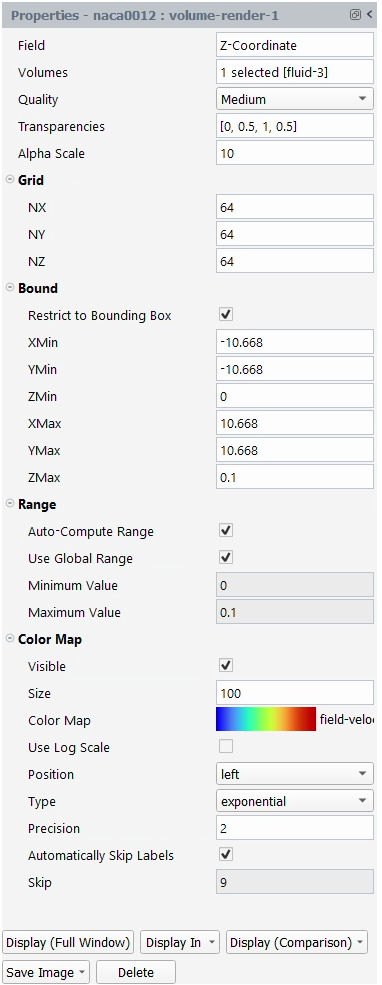
The following options are available when creating volume renders:
Field
Select the field variable that you want to use for creating the volume render.
Volumes
Select the volume(s) where you want to display the volume render.
Quality
Select the quality of the volume render.
Transparencies
Specify the transparencies to be used for different field values.
Alpha Scale
Specify to increase or decrease the transparency with lower values increasing transparency.
Grid
NX
Specify the number of clusters in the x-direction.
NY
Specify the number of clusters in the y-direction.
NZ
Specify the number of clusters in the z-direction.
Bound
Enable to specify bounding box extents.
Restrict to Bounding Box
Enable to specify bounding box extents.
XMin
Specify the bounding box extents (X Min).
YMin
Specify the bounding box extents (Y Min).
ZMin
Specify the bounding box extents (Z Min).
XMax
Specify the bounding box extents (X Max).
YMax
Specify the bounding box extents (Y Max).
ZMax
Specify the bounding box extents (Z Max).
Range
Set the range for the volume render:
Auto-Compute Range
Select to automatically determine the range of volume render values.
Use Global Range
Select to have the volume render display use data from the entire domain.
Minimum Value and Maximum Value
Allows you to set the range for the volume render data. These fields only apply when you disable Auto-Compute Range.
Color Map
Set the color map fields:
Visible
Select to have the color key displayed along the volume render display.
Size
Specify the number of levels in the color key for the volume render display, or keep the default value.
Color Map
Select a particular volume render color map scheme, or keep the default selection.
Use Log Scale
Select to have the volume render display use a logarithmic scale.
Position
Choose the position of the volume render color map in the graphics window, or use the default value.
Type
Choose the volume render color map presentation of data as general, exponential, or float.
Precision
Specify the numerical precision for the volume render color map data.
Automatically Skip Labels
Select to skip a certain number of labels (or show all) in the volume render.
Skip
Set a spacing on the colormap scale.
Periodic Instances allows you to create repeating copies, or periodic instances, of selected boundaries in the workspace. For example, if your current model represents a quarter of a sphere, you can apply rotational and/or translational properties to one or more periodic instances to display a full hemisphere. You can then use the periodic instances to better analyze the results of your simulation.
To create a periodic instance, right-click Periodic Instances in the Outline View tree and select New....
![]() Results → Graphics
→ Periodic
Instances
Results → Graphics
→ Periodic
Instances![]() New...
New...
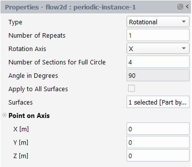
The following options are available when creating periodic instances:
Type
Select a rotational or translational periodicity.
Number of Repeats
Specify the number of times you want to repeat the periodic domain.
Rotation Axis
Select the direction vector (X,Y,Z) for the axis of rotation.
Number of Sections for Full Circle
Specify the number of segments that would form a full circle.
Angle in Degrees
Indicates the angle of rotation in degrees. This is equal to 360/Number of Sections for Full Circle.
Apply to All Surfaces
Select to apply the settings to all surfaces.
Surfaces
Select the surface(s) that you want to apply to the periodic instance.
Point on Axis
X [m]
Specify direction vector (X) for the axis of rotation.
Y [m]
Specify direction vector (Y) for the axis of rotation.
Z [m]
Specify direction vector (Z) for the axis of rotation.
Translational Vector
X [m]
Specify the distance in the X direction by which the domain is translated to create the periodic repeat.
Y [m]
Specify the distance in the Y direction by which the domain is translated to create the periodic repeat.
Z [m]
Specify the distance in the Z direction by which the domain is translated to create the periodic repeat.
Mirror Planes allows you define symmetry planes about which Graphics objects will be mirrored. The planes need to be axis-aligned.
To create a mirror planes, select Mirror Planes... under Graphics to open the Mirror Planes dialog.
![]() File
→ Graphics → Mirror
Planes...
File
→ Graphics → Mirror
Planes...
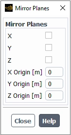
Specify whether the mirror plane will be oriented in the X, Y, or Z plane(s).
Specify the distance from the origin in the x, y, or z directions. Use the X Origin, Y Origin, or Z Origin fields.
You can visualize your changes as you make them in the dialog, and adjust the settings accordingly.
Material Assignment allows you define different materials to the various surfaces of your loaded dataset.
To assign a material, select Material Assignment... under Graphics to open the Assign Material To Surfaces dialog.
![]() File
→ Graphics → Material
Assignment...
File
→ Graphics → Material
Assignment...
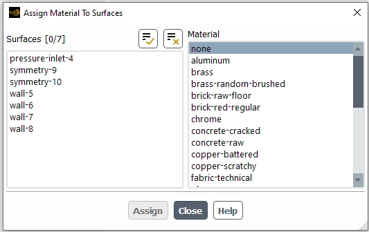
Select one or multiple Surfaces to assign the material to.
Select one Material from the list.
Press to assign the material to the respective surfaces.
You can draw vectors in the entire domain, or on selected surfaces. By default, one vector is drawn at the center of each cell (or at the center of each facet of a data surface), with the length and color of the arrows representing the velocity magnitude. The spacing, size, and coloring of the arrows can be modified, along with several other vector plot settings.
Note: Cell-center values are always used for vector plots as you cannot plot node-averaged values.
To create a vector plot, right-click Vectors in the Outline View tree and select New...
![]() Results → Graphics
→ Vectors...
Results → Graphics
→ Vectors...![]() New...
New...
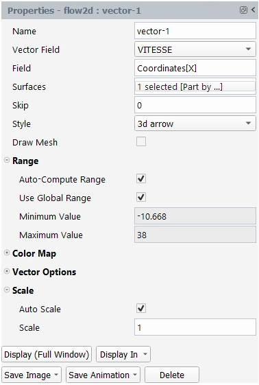
The following options are available when creating vector plots:
Name
(Optional) Enter a name for the vector object.
Vector Field
Select the vector quantity to be plotted.
Field
Specify the field variable you want to use to color the vectors.
Surfaces
Select the surfaces where you want the vectors displayed.
Skip
Specify the number of levels to include in the vector plot.
Style
Select a particular style for your vector markers.
Draw Mesh
Enable to draw the mesh with the vectors.
Overlayed Mesh
Choose the mesh object that you want to overlay upon the vectors.
Range
Set the range for the vector plot:
Auto-Compute Range
Automatically calculates the range for the vector colormap. When disabled, it allows you to clip the range to a specified Minimum and Maximum.
Use Global Range
Confirms that you are using the automatically computed range. However, if you do not want to use this range, you must disable Auto-Compute Range.
Minimum Value and Maximum Value
Allows you to set the range for the vector plot values. These fields only apply when you disable Auto-Compute Range.
ColorMap
Set the color map fields:
Visible
Toggle to have the color key displayed along with the vector display.
Size
Determines the size of the colormap.
Color Map
Specifies the colors to be used in the colormap display.
Use Log Scale
Uses a logarithmic scale.
Position
Determines where the colormap is located in the Graphics window.
Type
Lets you set whether the colormap follows a general, float, or exponential scale.
Precision
Lets you set the number of significant digits for the colormap.
Automatically Skip Labels
Select to skip a certain number of labels (or show all) in the vector color map.
Skip
Allows you to set a spacing on the colormap scale.
Vector Options
Select the desired vector options:
In Plane
Toggles the display of vector components in the plane of the selected surface. This feature is used for visualizing components that are normal to the flow.
Fixed Length
Sets all the vectors to the same length.
X Component
Toggles the display of the X component of vectors.
Y Component
Toggles the display of the Y component of vectors.
Z Component
Toggles the display of the Z component of vectors.
Head Scale
Allows you to control the size of the vector arrow head in relation to the length of the vector.
Color
Lets you specify a single color for all vectors.
Scale
Specify the vector scale from the default auto scale value:
Scale
Specify a value to increase or decrease the vector scale from the default auto scale value.
Pathlines are used to visualize the flow of massless particles in the problem domain. The particles are released from one or more surfaces that you have created as described in Surfaces. A line or rake surface (see Line Surfaces and Rake Surfaces) is most commonly used.
To create a pathline plot, right-click Pathlines in the Outline View tree and select New....
![]() Results → Graphics
→ Pathlines
Results → Graphics
→ Pathlines![]() New...
New...
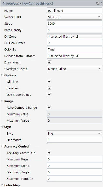
The following options are available when creating pathline plots:
Name
(Optional) Enter a name for the pathline object.
Vector Field
Select the vector quantity to be plotted.
Steps
Set the maximum number of steps that a particle can advance.
Path Density
Set the pathlines density to better visualize your pathlines.
On Zone
Select the zone(s) on which the particles are constrained to lie.
Oil Flow Offset
Specify the offset of pathlines that are constrained to lie on a particular boundary.
Color By
Specify the field variable you want to use to color the pathlines.
Release from Surfaces
Select the release point for the particles in the pathlines.
Draw Mesh
(Optional) Enable to display whichever mesh you select in the Overlayed Mesh drop-down list, which includes the outline and any defined mesh objects.
Overlayed Mesh
Choose the mesh object that you want to overlay upon the pathlines.
Options
Select the desired pathline options:
Oil Flow
Select to display pathlines that are constrained to lie on a particular boundary.
Reverse
Reverses the flow of the pathlines. The only difference is that the surfaces you select from the Release from surfaces list should actually be the final destination of the particles and not their source.
If you are interested in determining the source of a particle for which you know the final destination (for example, a particle that leaves the domain through an exit boundary), you can reverse the pathlines and follow them from their destination back to their source.
Use Node Values
Specifies that node values should be interpolated to compute the scalar field at a particle location.
Range
Set the range for the pathline plot:
Auto-Compute Range
Automatically calculates the range for the pathline colormap. When disabled, it allows you to clip the range to a specified Minimum and Maximum.
Minimum Value and Maximum Value
Allows you to set the range for the pathline plot values. These fields only apply when you disable Auto-Compute Range.
Style
Select how you want the pathlines displayed.
Line Width
Set the thickness of the pathlines.
Accuracy Control
Set the accuracy control:
Accuracy Control On
Enables/disables accuracy control.
Minimum Steps
Specifies the minimum number of steps a particle can advance.
Maximum Steps
Specifies the maximum number of steps a particle can advance.
Maximum Angle
Specifies the maximum angle of a particle.
Maximum Rotation
Specifies the maximum rotation of a particle.
ColorMap
Set the color map fields:
Visible
Toggle to have the color key displayed along with the pathline display.
Size
Determines the size of the colormap.
Color Map
Specifies the colors to be used in the colormap display.
Use Log Scale
Uses a logarithmic scale.
Position
Determines where the colormap is located in the Graphics window.
Type
Lets you set whether the colormap follows a general, float, or exponential scale.
Precision
Lets you set the number of significant digits for the colormap.
Automatically Skip Labels
Allows you to skip a certain number or show all labels in the pathline color map.
Skip
Allows you to set a spacing on the colormap scale.
Images can be saved in the workspace using the Save Picture dialog box, accessible from relevant Graphics objects (Contours, Vectors, etc.).
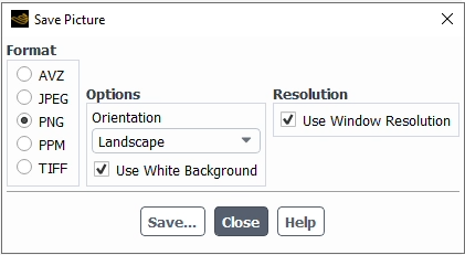
The following options are available when saving your images:
Format
Allows you to specify the saved image format as either AVZ, JPEG, PNG, PPM, or TIFF.
Options
Contains general animation options.
Orientation
Specify the orientation of the picture using the menu. If this option is turned on, the picture is made in mode; otherwise, it is made in mode.
Use White Background
If this option is enabled, the picture is saved with a white background.
Resolution
Specifies the resolution of the saved image.
Use Window Resolution
Uses the resolution of the current Graphics window when the image is saved.
Animations can be saved in the workspace using the Save Animations dialog box, accessible from relevant Graphics objects (Contours, Vectors, etc.).
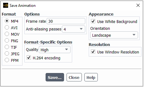
The following options are available when saving your animations:
Format
Allows you to specify the saved animation format as either MP4 (default), AVI, MOV, PNG, TIF, JPEG, or PPM.
Options
Contains general animation options.
Frame Rate
Specify rate of the frames (in frames per second, fps) to be set for the animation to be recorded. Generally, the default is 30fp (for MP4, AVI, or MOV formats).
Anti-aliasing Passes
Specify the number of anti-aliasing passes required to smooth out edges and distortions.
Fomat-Specific Options
Contains options that are specific to the chosen animation format.
Quality
(MP4) Allows you to control the quality and resolution for the animation sequence.
H.264 encoding
(MP4) Allows you to control the encoding for the animation sequence.
Bit rate
(AVI and MOV) Allows you to control the bit rate for the animation sequence.
Compression
(AVI, PNG, TIF) Allows you to control the compression method for the animation sequence.
JPEG Quality
(JPEG) Allows you to control the compression rate (0-100) for the animation sequence.
PPM Format
(PPM) Allows you to save the animation files as Binary (Default) or ASCII.
Appearance
Specifies the general look of the saved animation.
Use White Background
Allows you to save animations with a white background and a black foreground.
Orientation
Controls the orientation of the animation as either Landscape or Portrait.
Resolution
Specifies the resolution of the saved animation.
Use Window Resolution
Uses the resolution of the current Graphics window when the image is saved.
You can create plots to visualize your results.
The following plots are available:
You can create 2D XY plots of your results for analyzing one variable with respect to another variable.
To create an XY plot, right-click XY Plots in the Outline View tree and select New....
![]() Results → Plots
→ XY
Plots
Results → Plots
→ XY
Plots![]() New...
New...
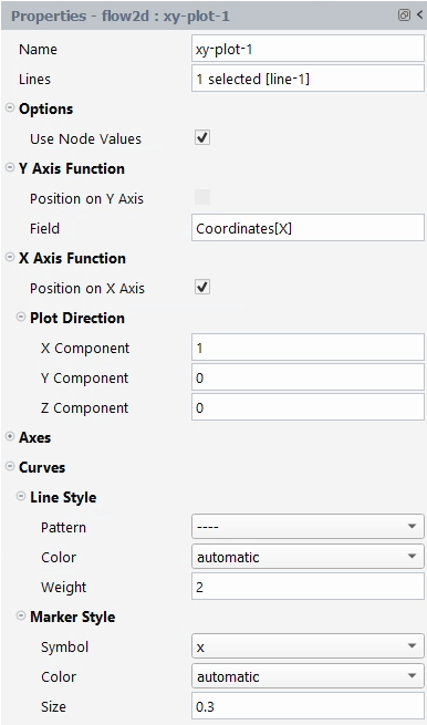
The following options are available when creating XY plots:
Name
(Optional) Enter a name for the XY Plot.
Lines
Select the surfaces where the plot parameters apply.
Options
Use Node Values
Specify whether the values should be calculated using cell-centered values alone or if they should also include node values.
Y Axis Function
Position on Y Axis
Enable to plot position on the y-axis.
Field
Specify the field variable you want to display for the Y axis.
Alternatively, you can set the Y axis to be the location on the Y axis, by enabling Position on Y Axis.
X Axis Function
Position on X Axis
Enable to plot position on the x-axis.
Plot Direction
Specify the Plot Direction by confirming the values for the X Component, Y Component, and Z Component.
Axes
(Optional) Define axes labels and options:
X Axis
Label
Enter a label for the x-axis.
Options
Choose the axis options:
Log
Axis values are displayed on a logarithmic scale.
Auto Range
Axis minimum, maximum, and increment are computed automatically.
Major Rules
Draw lines through the plot at each major increment.
Minor Rules
Draw lines through the plot at each minor increment.
Number Format
Set the number format for how axis values are displayed.
Type
Select the desired number output type from the drop-down list.
Precision
Set the precision to control the number of significant digits.
MajorRules
Color
Select the color of major tick marks.
Weight
Specify the thickness of major tick marks.
MinorRules
Color
Select the color of minor tick marks.
Weight
Specify the thickness of minor tick marks.
Set the axis Range by entering values for Minimum and Maximum. Note that these values are only used when the Auto Range option is disabled.
Y Axis
Set up the Y Axis by defining the settings as desired. The inputs fields are equivalent to the ones available for the X axis, as described above.
Curves
(Optional) Specify the curves properties.
Line Style
For lines (under Line Style) you can control the Pattern, Color, and Weight (equivalent to line thickness).
Marker Style
For markers (under Marker Style), you can control the Symbol, Color, and Size.
Click to plot the data.
You can also plot or save the plot data to a file or as an image, by clicking , or respectively.
Transient plots are a valuable post-processing tool that allow you to use study time-dependant aspects of your simulation.
To create a transient plot, right-click Transient Plots in the Outline View tree and select New....
![]() Results → Graphics
→ Transient
Plots
Results → Graphics
→ Transient
Plots![]() New...
New...
The following options are available when creating a transient plot:
Name
(Optional) Enter a name for the transient object.
Reports
Select the reports you would like to include in the transient plot.
Title
Enter a title for the transient plot.
X Axis
Specify the variable you want to apply to the x-axis for the transient plot.
X Axis Label
Specify the x-axis label you want to apply to the transient plot.
Y Axis Label
Specify the y-axis label you want to apply to the transient plot.
Timestep Selection
Set the timestep selection for the transient plot:
Option
Choose the timestep selection option for plotting, printing to console or exporting to file.
Begin Time [s]
Specify the start time for plotting, printing to console or exporting to file.
End Time [s]
Specify the end time for plotting, printing to console or exporting to file.
Time Increment [s]
Specify the time increment to use for plotting, printing to console or exporting to file.
Axes
X Axis
Options
Choose the axis options:
Log
Axis values are displayed on a logarithmic scale.
Auto Range
Axis minimum, maximum, and increment are computed automatically.
Major Rules
Draw lines through the plot at each major increment.
Minor Rules
Draw lines through the plot at each minor increment.
Number Format
Set the number format for how axis values are displayed.
Type
Select the desired number output type from the drop-down list.
Precision
Set the precision to control the number of significant digits.
MajorRules
Color
Select the color of major tick marks.
Weight
Specify the thickness of major tick marks.
MinorRules
Color
Select the color of minor tick marks.
Weight
Specify the thickness of minor tick marks.
Set the axis Range by entering values for Minimum and Maximum. Note that these values are only used when the Auto Range option is disabled.
Y Axis
Set up the Y Axis by defining the settings as desired. The inputs fields are equivalent to the ones available for the X axis, as described above.
Curves
(Optional) Specify the curves properties.
Line Style
For lines (under Line Style) you can control the Pattern, Color, and Weight (equivalent to line thickness).
Marker Style
For markers (under Marker Style), you can control the Symbol, Color, and Size.
Once you have set your properties:
Click to create a hard copy of the plot.
Click to display the plot in the Graphics window.
Click to save the report in another format.
Click Delete to remove the plot.
Click to save the plot as an image.
Click to pick and choose the reports files that your plot is comprised of.
Transient report data can be exported using the Export dialog, accessible from the relevant transient report property page.
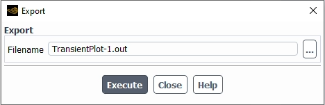
For Filename, use the  button or
enter the name and location of the relevant report file(s) that you want to
export.
button or
enter the name and location of the relevant report file(s) that you want to
export.
Data from any number of report files can be added to and removed from a transient plot using the Report Files dialog, accessible from the relevant transient report property page.
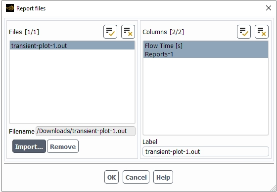
Use Import... to load report files (indicated in the Filename field) into the Files column. Relevant data is then listed under Columns, with its default Label that can be changed accordingly. Use to remove a selected file(s) from the report.
Static reports are available for computation of various post-processing quantities.
![]() Results → Reports
→ New...
Results → Reports
→ New...
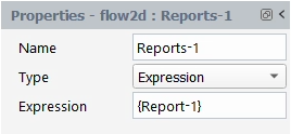
Note: For expression based reports, the following operators are allowed:--, +, -, *, /, **.
Expressions can be functions of other report objects and/or numerical
constants. To refer to another report, the report name should be enclosed in
curly brackets without any spaces, for example
{Report-1}.
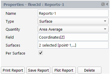
The following options are available when creating reports:
Name
(Optional) Enter a name for the report.
Type
Choose the type of report as either a Surface, Volume or Expression report.
Quantity
Choose the Surface quantity that you want to report.
Area Average
Area average of the specified variable over the selected surface(s).
Area
Area of the selected surfaces.
Facet Average
Facet average of the specified variable over the selected surface(s).
Facet Maximum
Facet maximum of the specified variable over the selected surface(s).
Facet Minimum
Facet minimum of the specified variable over the selected surface(s).
Flow Rate
Flow rate of the specified variable over the selected surface(s).
Mass Flow Rate
Mass flow rate of the specified variable over the selected surface(s).
Standard Deviation
Standard deviation of the specified variable over the selected surface(s).
Surface Integral
Surface integral of the specified variable over the selected surface(s).
Surface Mass Average
Surface mass average of the specified variable over the selected surface(s).
Surface Sum
Surface sum of the specified variable over the selected surface(s).
Vertex Average
Vertex average of the specified variable over the selected surface(s).
Vertex Maximum
Vertex maximum of the specified variable over the selected surface(s).
Vertex Minimum
Vertex minimum of the specified variable over the selected surface(s).
Volume Flow Rate
Volume flow rate of the specified variable over the selected surface(s).
Choose the Volume quantity that you want to report.
Average
Average of the specified variable over the selected surface(s).
Mass
Mass of the specified variable over the selected surface(s).
Mass Integral
Mass Integral of the specified variable over the selected surface(s).
Maximum
Maximum of the specified variable over the selected surface(s).
Minimum
Minimum of the specified variable over the selected surface(s).
Volume
Volume of the specified variable over the selected surface(s).
Volume Average
Volume Average of the specified variable over the selected surface(s).
Volume Integral
Volume Integral of the specified variable over the selected surface(s).
Volume Mass Average
Volume Mass Average of the specified variable over the selected surface(s).
Volume Sum
Volume Sum of the specified variable over the selected surface(s).
Volume Fraction Field
This is an optional entry which can be used to specify the volume fraction to be used when calculating a report. This field is available for the following Quantity types:
Mass Integral
Flow Rate
Surface Mass Average
Mass
Volume
Volume Sum
Volume Mass Average
Volume Integral
Volume Flow Rate
Mass Flow Rate
Volume Average
Choose an Expression to report.
Specify an expression (functions of other report objects and/or numerical constants) to define your property field. To refer to another report, the report name should be enclosed in curly brackets without any spaces, for example
{Report-1}.Field
Select the field variable to be used in the surface or volume integrations.
Surfaces/Volumes
Select the surfaces/volumes used in computing the report definition.
Per Surface/Per Volume
Select to include individual surfaces or volumes.
Once a report is created, click and the result is printed in the Console. Click and the result is saved to a file and location of your choice. Click and the result is printed in the Graphics window.
Reports can be printed in the workspace using the Print Report dialog box, accessible from the relevant report object property page.
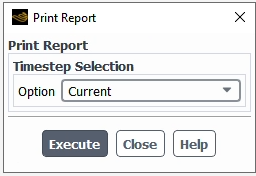
The following options are available when printing your reports:
Timestep Selection
Indicate specific details of the time step (Current, First, Last, All, or specify the starting point, the ending point and a particular increment.
Reports can be saved in the workspace using the Save Report dialog box, accessible from relevant report object property page.
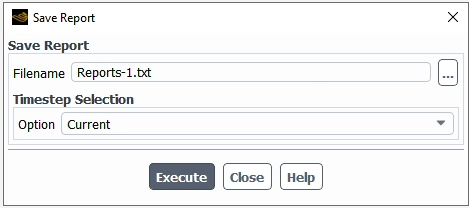
The following options are available when saving your reports:
Filename
Specify the name and location of the report that you want to save.
Option
Indicate specific details of the time step (Current, First, Last, All, or specify the starting point, the ending point and a particular increment.
Reports can be plotted in the workspace using the Plot Report dialog box, accessible from the relevant report object property page.
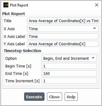
The following options are available when plotting your reports:
Title
Specify the title you want to apply to the plot report
X Axis
Specify the variable you want to apply to the x-axis for the plot report.
X Axis Label
Specify the title you want to apply to the x-axis for the plot report.
Y Axis Label
Specify the title you want to apply to the y-axis for the plot report.
Timestep Selection
Indicate specific details of the plot report time step (Current, First, Last, All, or specify the starting point, the ending point and a particular increment.