


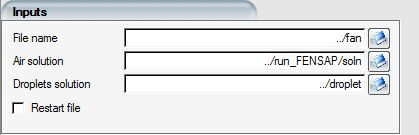
This section allows the configuration of the input files and the various options pertaining to the selection of the various icing models provided by ICE3D.
The grid and air/droplets/crystals solution files should be selected before setting up the input parameters since some of these, for example boundary conditions, which are grid-dependent. Activate the check box Vapor solution and assign its file to use DROP3D-calculated local surface vapor pressure in the ICE3D computation.
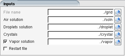
The grid file should be assigned using the grid icon in the run window, however it can also be assigned in this window. The grid file is then read to detect any changes to the boundary conditions.
Note: To use vapor solution for icing computations, air solution must be obtained with adiabatic walls and EID calculation (Compute EID (Extended Icing Data)) should be enabled.
ICE3D can be restarted from a previous ice.grid displaced ice grid file and corresponding swimsol solution file. Click in the Restart file box and use the browse window to assign the grid and solution file.
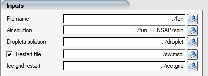
Alternatively, right-click the ICE3D configuration icon in the project window, select Options in the menu and chose the Use restart solution option.
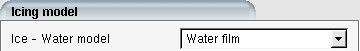
The Icing model panel provides the options for the ice accretion, surface displacement, and roughness output models.
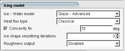
Select the option Glaze - Advanced in the Ice - Water model section to solve the three governing equations and integrate the glaze ice accretion in time. In this case, both the shear stress and heat flux from the air solution should be provided.
FENSAP computes heat fluxes in two different ways: Classical, which is based on temperature gradients on the walls, or Gresho, which is based on Gresho’s Consistent Galerkin formulation. Select either one of these two flux types in the Heat flux type box. Both Classical and Gresho fluxes are 2nd order accurate and should give very similar results. However, Gresho fluxes can exhibit some oscillations if the surface grid is uneven or coarse. For accurate heat fluxes, the recommended boundary layer grid spacing is: first element size 1e-6 m chords of an airfoil, with a growth ratio of 1.1.
In the special case of very low temperatures and low speeds, when the reference stagnation temperature is well below freezing, the ice accretion problem can be simplified with the Rime ice option, in which case all droplets are assumed to freeze on impact (no runback).
The energy equation is not solved, and the wall temperature remains at the recovery temperature. Inviscid air flow solutions can be used for this type of simulation without any shear stress or heat flux data. Heat flux type will be grayed out since it is not used.
The Volume - Based growth model supports a concavity check algorithm to help prevent the ice surface mesh from folding during growth. A minimum angle between the node normal and the adjacent faces can be enforced. The artificial displacement added to a surface grid node by concavity fixing is limited to maximum physical displacement of neighboring grid nodes. Pre-existing concave parts of the mesh will not be artificially displaced if there is no icing taking place in the surrounding nodes. This option should always be turned on (default).
This option can be used to generate smoother ice shapes to help with mesh displacement and remeshing processes. In internal icing cases, such as engine inlet guide vanes, the growth of ice surface at the shroud/blade intersection can be especially problematic, and lead to premature failures in the remeshing process. Applying smoothing can delay or entirely avoid such failures, without a significant loss in the overall ice shape definition.
The ice shape smoothing is done by relocating the nodal accumulated ice growth between neighboring nodes conservatively using area weighted averaging, prior to computing surface node displacement. It is not a smoothing process on the nodal coordinates, but the ice mass distribution itself. The process can be iterated to increase the level of smoothing. By default, it is set to 0.
When the Beading model is activated, a sand-grain roughness distribution is computed over the contaminated surfaces to model the roughness of the frozen ice beads. The roughness distribution is a function of location as well as ice accretion time. The roughness distribution greatly affects the surface heat fluxes and shear stresses, and therefore has a considerable impact on the quality of the final ice shape in multishot calculations. The surface sand-grain roughness distribution is automatically written to the roughness.dat file when beading is enabled. The roughness.dat file will then be read automatically by FENSAP at the beginning of the next shot.
Note: When the Beading model is selected, the sand-grain roughness output is automatically activated.
The beading model is used to analytically calculate the evolution of the ice roughness.
ICE3D assumes the presence of a continuous film of water when glaze conditions exist on the contaminated surface. Experimental evidence however indicates that when droplets impact on a surface they tend to form beads that grow in time before running back and freezing as nearly-hemispherical ice caps.
The Beading model can predict sand-grain roughness height on the surface caused by moving and freezing beads. The local bead height changes not only in space but also in time, therefore beading works best as a component of an unsteady or quasi-steady simulation, since it affects the heat fluxes and therefore the growth rate of the accreting ice.
Furthermore, the Beading model removes any empiricism in the selection of surface sand-grain roughness and therefore considerably enriches the level of physical modeling and simulation accuracy obtainable with ICE3D.

To select this model, choose Activated in the Beading box. The Beading model is only available in the Glaze - Advanced mode. The surface sand-grain roughness distribution file roughness.dat, used by FENSAP to simulate variable surface roughness, can be written by choosing Roughness output: From beading in the Icing model menu shown in Sand-Grain Roughness Output.

Note: This option completely eliminates the guesswork of selecting the appropriate roughness height and dramatically improves the accuracy of multishot calculations.
To take advantage of the roughness output from beading, multishot calculations are necessary in order to make use of this roughness distribution for the next shot.
If icing shots are long, for example, 1 minute or more, the first shot may still need to be solved with an initial roughness applied to the surface if the expected rate of ice accretion is high. The current best practice is to use 0.5mm which has shown good agreement with experimental ice shapes on ~0.5m-chord airfoils. For smaller geometries with sharper leading edges, 0.5mm may be too high and favor a more rime-like result. For such cases, it is recommended to use shorter shots with “no roughness” for the first shot.
For cases with rotating walls and/or high-speed flows, where the wall recovery temperature cannot be easily related to the free stream reference temperature using a recovery factor, the flow solution should be calculated using adiabatic walls. In this case heat fluxes and wall heat transfer coefficients need to be calculated with an alternative method called EID (extended icing data). This is a proprietary technology that solves an iterative system to extract heat transfer coefficients from adiabatic air flow solutions. Uncommon ice shapes like beak-ice observed at Mach ~ 0.6 range can be captured with the use of EID. For such shapes usually the stagnation temperature is several degrees above freezing, while the free stream static temperature is well below freezing. EID is required to correctly simulate icing on rotating components like helicopter and turbomachine rotors.
When providing an adiabatic flow solution to ICE3D, enable EID by selecting in the Compute EID drop-down:

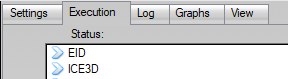
When starting the icing calculation with EID enabled, the Execution window first displays the EID run, followed by ICE3D:
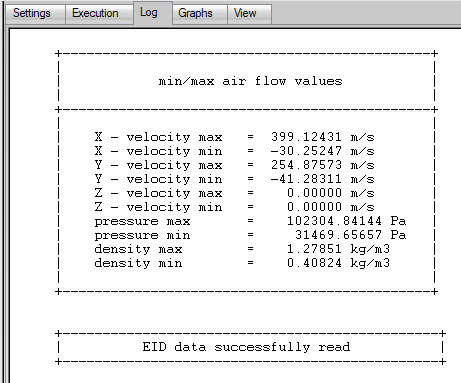
ICE3D log should show a message for successful processing of EID at the start of the calculations:
Computation of EID will produce several files in the ICE3D run directory, such as soln.eid and converg.eid. The former is loaded by ICE3D to bring in the EID solution. The latter can be used to verify convergence of the EID iterations.
Important: The solution produced by Fluent and CFX will be converted by FENSAP-ICE. It is necessary to provide all the information requested regarding the reference freestream conditions. These reference values must also be used in the ICE3D Conditions panel.
The same procedure regarding the initialization of the reference values must also be followed when converting the solution and running ICE3D in batch mode.
EID makes use of laminar viscosity, laminar conductivity, and turbulent viscosity. These fields must be present in the supplied air solution file for EID to function properly. If laminar conductivity is missing, it will be calculated from the local temperature using Sutherland’s law.
Recovery temperatures of rough and smooth walls can be very different at high speeds. It is recommended starting such multishot icing calculations with smooth walls when using EID, and build the ice roughness progressively using the beading model.
The ice crystal bouncing models determine the amount of crystals that contribute to the icing calculation. There are two options available.
The model can be accessed in the Model panel of ICE3D when a crystal solution is present. The NTI bouncing model determines the amount of crystals that stick based on local surface conditions, such as impact velocity, crystal size and film height. The model also includes an optional feature to account for crystal erosion effects on ice accreting surfaces.
The NRC Model calculates the sticking fraction based on the liquid water content to total water content (LWC/TWC) ratio hitting the surface. The model can be selected by choosing the NRC Bouncing Model option in the Model panel of ICE3D.
Note: The Crystal erosion is an option only available within the NTI bouncing model.
The Custom bouncing model is a feature developed to provide flexibility for you to define their own sticking fraction within the crystal icing framework. The model requires you to create a User Defined File (UDF) that calculates the sticking fraction at each nodal location on the surface grid. The language syntax for FENSAP-ICE UDF’s can be found in UDF Syntax. The model can be selected by choosing Custom Sticking Model option from the Model panel of ICE3D.
Selecting the Custom Sticking model allows you to construct a sticking fraction for crystals impacting a surface. Once created, the UDF must be chosen in the User Defined Functions section in the Model panel.
Note: UDF template files can be found in the fensapice/data/udf directory of the FENSAP-ICE installation directory.
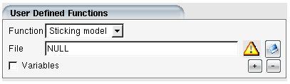
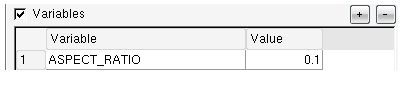
Constants that are used in the UDF file can be defined by adding a checkmark next to the Variables option. For example, ASPECT_RATIO, a variable that defines crystal geometric properties can be added and assigned a static value as follows:
A small program is prepared by you in a text file. The program runs on each node, with each iteration of the simulation ICE3D.
Different physical variables (velocity vectors, crystal and droplet
concentration, normal surface vectors) are already available to you and can be
used if desired. The language defining the UDF is made of simple expressions
close to the C language.
The basic rules are:
A line beginning with
#is a comment and will be ignoredEach expression must be terminated with a semicolon (;)
An arbitrary number of spaces and empty lines can be used
All variables are floating point (double precision)
Local variables can be declared, the declaration syntax requires a
@, the structure is a statement:@VARIABLE = VALUE;The program must end with a
return 0
An expression is a combination of basic arithmetic operators

With the following additions
 : Power
 : Modulo, floating point
Logical operators are

The digital logic operation result is 0 (false) or 1 (true).
Priority between operators is similar to C language.
Parentheses can be used freely and are preferable to make the code less
ambiguous.
Math
sqrt () cos () sin () tan () acos () asin () atan () atan2 (,) exp
                        ()
Trigonometric functions use radians.
Values
fabs () - absolute value
min(val1, val2) – minimum of value 1 and 2
max (val1, val2) – maximum of value 1 and 2
round ()
floor ()
ceil ()
sqrt ()
cos ()
sin ()
tan ()
acos ()
asin ()
atan ()
atan2 ()
exp ()
Utilities
print ( "Text") print (val)
File Access
fileData1D (value, "filename")
Use this feature to interpolate within values contained in a file. The file
contains two columns. The call to fileData1D returns an
interpolated value in the 2nd column, by providing a value contained within the
range of the 1st column.
This can be used to represent experimental data curve or function too complex to be easily defined with an equation.
File format for fileData1D:
npoints
variable value
variable value
variable value
variable value
Example 6.1: fileData1D File Format
5
0.5 291.75
0.6 293.4
0.73 295.9935
0.88 299.616
1.2 309.6
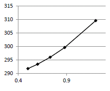
Given a value of 0.55,
fileData1D(0.55,"data.txt")
returns 292.595 based on linear
interpolation of values corresponding to
0.5(291.75) and
0.6(293.4)
When starting ICE3D, the UDF will be read and syntax will be checked. If the syntax is invalid, ICE3D will stop and a message like the following will be visible in the execution log.
Expression syntax error: invalid operands
ERROR: execution error
To identify a problem in writing the program, it is suggested to review the problematic lines to isolate it.
To check the steps of the calculation, it is possible to display the
calculated values in the UDF using the print
() function. Since the program is being executed on each node at
each iteration (and each CPU), it is better to debug using 1 CPU and a smaller
mesh.
Example 6.2: Calculation of Steps
@REI = DENS *VELMAG*DIAM / MU_A;
print ( "REI value:");
print (REI);
Would print for each evaluated node:
PRINT: "REI Value" (string)
PRINT: 57.4614 (float)
PRINT: "REI Value" (string)
PRINT: 57.2643 (float)
This example is based on 2014 NRC sticking model:
# CUSTOM UDF TEMPLATE FOR COMPUTING STICKING FRACTION
# DIMENSIONAL VARIABLES THAT CAN BE USED
# CRYSTALS
# -------------
# ICC - LOCAL CRYSTAL CONTENT (kg/m3)
# LWC - LOCAL LIQUID WATER CONTENT (kg/m3)
# TWC - LOCAL TOTAL WATER CONTENT (kg/m3)
# XVEL - DIMENSIONAL CRYSTAL VELOCITY X
# YVEL - DIMENSIONAL CRYSTAL VELOCITY Y
# ZVEL - DIMENSIONAL CRYSTAL VELOCITY Z
# DIAM - ICED DIAMETER/SIZE
# NORMX - SURFACE NORMAL X
# NORMY - SURFACE NORMAL Y
# NORMZ - SURFACE NORMAL Z
# CONSTANTS
# ----------------
# VELINF - REFERENCE FREESTREAM VELOCITY
# INPUTS FOR NRC STICKING FRACTION
# ------------------------------------------
# NFACT - 2016 NRC COEFFICIENT
# KPOWER - EROSION FUNCTION COEFFICIENTS
# LPOWER - EROSION FUNCTION COEFFICIENTS
# CONSTA - EROSION FUNCTION COEFFICIENTS
# CONSTB - EROSION FUNCTION COEFFICIENTS
# NSTAG - STAGNATION STICKING EFFICIENCY(INTERPOLATED FROM FILE INPUT)
# REQUIRED OUTPUTS
# ----------------------------
# STFRACTION - STICKING FRACTION FOR CRYSTALS
@PI = 3.14159265359;
@RATIO = LWC/TWC;
#STAGNATION POINT STICKING EFFICIENCY
#-------------------------------------
@NSTAG = fileData1D(RATIO,"nrc_stick.txt");
#ANGLE BETWEEN SURFACE NORMAL AND IMPACT VELOCITY
#------------------------------------------------
@VNORM = (XVEL*NORMX + YVEL*NORMY + ZVEL*NORMZ);
@VELMAG = (XVEL^2 + YVEL^2 + ZVEL^2)^0.5;
if( VNORM < 0.0 ) {
 VNORM = -VNORM;
};
@PSI = acos( VNORM/VELMAG );
#2014 NRC STICKING FRACTION COEFFICIENTS
#---------------------------------------
@KPOWER = 0.0;
@LPOWER = 1.5;
@SINFAC = 1.0;
@CONSTA = 1.0 - NSTAG;
@CONSTB = 0.578/VELINF^LPOWER;
# FLUX REDUCTION FACTOR
#-----------------------------------
if( TWC <= 0.004 ) {
 @A_F = 0.0;
 }
else if( TWC <= 0.012 ) {
 @A_F = -0.1425 + 47.292*TWC - 1979.167*TWC^2;
 }
else {
 @A_F = 0.140;
 };
#EROSION REDUCTION FACTOR DUE TO FLUX INTERFERENCE
#-------------------------------------------------------------------------------
@EROFACT = 1.0 - A_F*sin(PSI);
if(EROFACT < 0.86 ){
 EROFACT = 0.86;
};
if(EROFACT > 1.0 ){
 EROFACT = 1.0;
};
#EROSION FUNCTION
#----------------------------
@EROFUNC = SINFAC*( CONSTA*(VELINF*cos(PSI))^KPOWER + CONSTB*(VELINF*sin(PSI))^LPOWER );
#STICKING FRACTION
#---------------------------
STFRACTION = 1.0 - EROFACT*EROFUNC;
return 0Rotating components, such as engine spinners, fan blades, propeller blades and helicopter rotors can undergo ice shedding where strong centrifugal forces on the ice can eventually reach a critical point, overcoming adhesive forces between ice and the surface.
Ice can crack and detach from a surface according to different failure modes. The adhesive failure mode involves the detachment of the entire ice layer from the surface, while the cohesive failure mode begins with the formation of a crack, followed by the fracture and delamination of an isolated ice piece within the ice layer. This section will focus on the modeling of ice shedding in a mixed failure mode that accounts for both adhesive failure at the ice-metal interface as well as cohesive failure within the ice volume subject to centrifugal loads.

The ice shedding model is provided within ICE3D or ICE3D-TURBO. It is activated by enabling the option in the model panel of the run. ICE3D evaluates the shedding of ice by automatically interfacing the ice accretion to an internal stress calculation in the ice volume. The stress solver is triggered at the solution output write-out interval specified by the user.
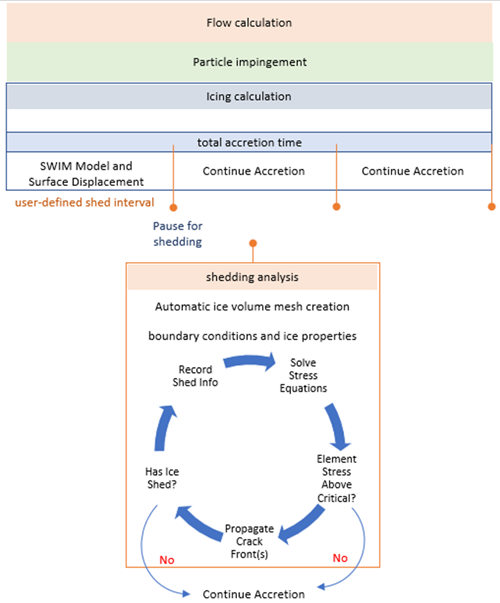
During the stress calculation, the crack propagation and determination of shed fragments, their CG positions as radii, mass and ice remaining are determined. Centrifugal forces in the ice must overcome aerodynamic, adhesive and cohesive stresses for the ice to shed. A flowchart of the entire process within the ICE3D calculation has been shown in the figure above.
The adhesive strength of ice to the accreting surface depends on the type of surface defined in the Ice-Surface interface options.
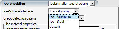
, and adhesive strengths can be defined. and average values are based on available literature.
| Ice aluminum | 0.3 MPa |
| Ice steel | 10 MPa |
The interface model also includes a functional dependence with surface
temperature, as adhesion strength is known to vary with temperature. For
example, the adhesive tensile strength of steel to ice with respect to surface
temperature  is:
is:

A Custom UDF adhesive strength can also be defined. A template file with thermally varying normal and shear adhesion has been defined below:

In addition to the adhesive strength, the aerodynamic forces due to pressure and shear, as well as body forces due to centrifugal forces are used in a force balance calculation to determine if ice delaminates off the surface.
Note: UDF template files can be found in the fensapice/data/udf directory of the FENSAP-ICE installation directory.
# CUSTOM UDF TEMPLATE FOR COMPUTING STICKING FRACTION
# DIMENSIONAL VARIABLES THAT CAN BE USED
# SURFACE PARAMETER INPUTS FROM ICE3D
# -----------------------------------------------------------
# TEMP	- LOCAL ICING SURFACE TEMPERATURE (Celsius)
# XCOORD - X COORDINATE (m)
# YCOORD - Y COORDINATE (m)
# ZCOORD - Z COORDINATE (m)
# RADIUS - RADIAL COORDINATE (m)
# THETA - THETA COORDINATE (degrees)
#
# REQUIRED OUTPUTS TO ICE3D
# -----------------------------------------
# FADHES_N - TENSILE ADHESIVE STRENGTH ( Pa )
# FADHES_T - SHEAR ADHESIVE STRENGTH ( Pa )
# ADHESIVE ICE-INTERFACE STRENGTH TEMPLATE
# -----------------------------------------------------------------
FADHES_N = 0.0;
FADHES_T = 0.0;
if( TEMP <= -10.5 )
{
    FADHES_N = 1000*(-TEMP + 450.0);
    FADHES_T = FADHES_N*0.181140;
}
else if( TEMP <= 0.0 )
{
FADHES_N = 1000*(-40.0*TEMP + 60.0);
FADHES_T = FADHES_N*(0.000070*TEMP^3 + 0.0006*TEMP^2 - 0.0147*TEMP + 0.0242);
};
return 0The displacement of the ice structure can be described by the Cauchy-Navier equation:

where  are the components of the displacement vector and
 is the resultant body force on the ice due to centrifugal
forces. The two parameters
is the resultant body force on the ice due to centrifugal
forces. The two parameters  and
and  are determined by Young’s modulus
  and Poisson’s ratio
  .
.


The displacement on each node allows the calculation of 6 stress tensors in the element:

The stress tensors can then be used to evaluate the maximum principal stress
 in the element. There are two options: or to evaluate
potential cracking in the ice structure.
in the element. There are two options: or to evaluate
potential cracking in the ice structure.
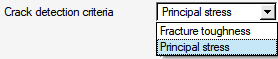
The option uses the user defined cohesive tensile strength of ice to select elements for cracking.

is also provided as an option and is used to evaluate a criteria to compare the calculated principal stress:


Where  is the work of fracture,
  is the user defined fracture toughness and
  is the characteristic length of the element. In general,
fracture toughness is used for ductile materials.
is the characteristic length of the element. In general,
fracture toughness is used for ductile materials.
Cracking occurs if the calculated maximum principal stress in an element exceeds the critical stress

Principal stress is the preferred method over fracture toughness for ice crack propagation simulation, as ice is a brittle material that exhibits a low-strain rate.
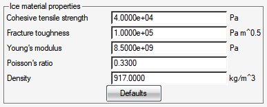
For the ice shedding model, ice is assumed to be an isotropic solid material with mechanical properties within the linear elastic regime during in-flight icing encounters. The ice properties shown below are based on average literature values and maybe changed if user data is available.
The out panel in ICE3D allows the user to control the frequency of the shedding analysis through the Shedding every printouts option. The user can specify the shedding interval as a multiple of the time between solution printouts. For example, if the Time between solution output of 1 second and Shedding every 10 printouts is specified, then the shedding analysis is carried out every 10 seconds.
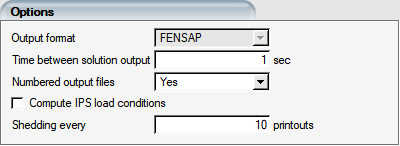
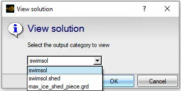
You are encouraged to activate the Numbered output files option to see how the shedding ice solution evolves with time. The following shedding files will be produced as outputs during the calculation:
swimsol.shed - ice solution file post-shed
ice.grid.shed - ice grid file post-shed
max_ice_shed_piece.grd – largest ice volume that shed in the time period
iceshed.log – No. of fragments that shed, mass of each fragment, COG radial distance from centerline for each shedding instance
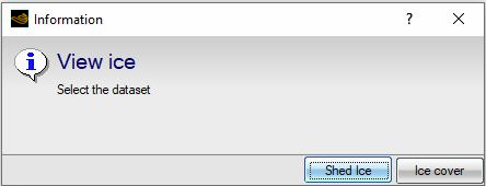
The and buttons in the execution panel of the ice shedding run allow you to view the shed solution files:
Two different types of body force can be applied during simulations.
The effect of gravity can be added to the water film velocity. To do so, select in the list of body forces.
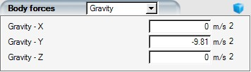
Enter the components of the gravity vector in the body force window. Select None to neglect the impact of gravity (typical of most icing applications).
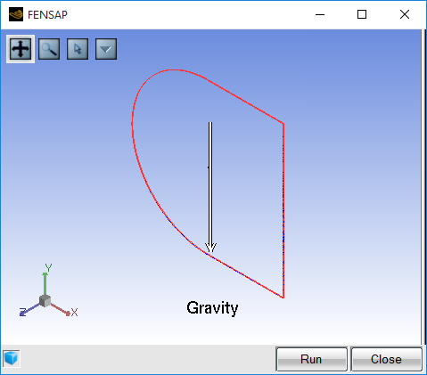
Click the display icon ![]() to display the gravity vector in the graphical window. To
remove the gravity vector from the graphical window, click another time on this
icon.
to display the gravity vector in the graphical window. To
remove the gravity vector from the graphical window, click another time on this
icon.
For ice accretion in a rotating frame of reference, select the Rotation speed option in the Body forces section. See Rotating Frame of Reference for more details.
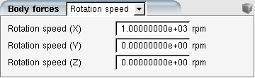
The three components of the rotation speed Ω used for the airflow and droplet calculation should then be entered in the appropriate boxes.
If at least one of the three components is non-zero, a reminder that the frame of reference has been switched to Relative will appear at the bottom of the window.

Note: If the ICE3D config icon is initialized by dragging & dropping the DROP3D config icon, the rotational components will be initialized automatically.