


All FENSAP-ICE modules solve systems of partial differential equation and therefore require sets of suitable boundary conditions.
The Boundary conditions panel lists all boundary condition indices present in the grid file. The possible indices and their usage are:
| Index | Boundary Condition Type |
|---|---|
| BC_1000 to BC_1999 | Inlet/Far field |
| BC_2000 to BC_2999 | Wall |
| BC_3000 to BC_3999 | Outlet |
| BC_4000 | General |
| BC_4100 | X-symmetry |
| BC_4200 | Y-symmetry |
| BC_4300 | Z-symmetry |
| BC_5000 to BC_5099 | Periodic – translational and rotational |
| BC_6000 to BC_6999 | Internal surface – actuator disks, screens, heater pads, custom post processing, etc... |
| BC_7000 to BC_7999 | Non-conformal interfaces, Rotor/fuselage gap boundaries |
Inlets, walls, outlets and internal surfaces have subtypes that need to be set in their respective menus, which are explained in the sections below.
The name of each boundary condition tag can be modified in the Label box. The name of a boundary is for bookkeeping purposes only, it does not change the type nor the function of the boundary. To view the boundary surface in the graphical window, check the square box next to its label.
Multiple boundary conditions can be selected as a group with the Shift or Ctrl keys. If the visibility check box is toggled, the action will apply to the whole selection. If the selected boundary conditions are of the same type, such as inlet, wall or outlet, any setting changes will be applied to all the selected boundary conditions.
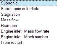
Inlet boundary indices can range from 1,000 to 1,999. Indices ranging from 10 to 19 are still supported for backward compatibility but are converted to the four-digit format. Several inlet types are supported:
In general, velocity components and static temperature are imposed at subsonic inlets and static pressure specification is done on subsonic exits. The different inlet types listed below recast the formulation to allow imposition of these variables through total conditions, mass flow rates, or Mach number.
To display the boundary velocity vector in the graphical window, Click the display icon:
If a turbulence model is selected, an inlet profile of turbulent viscosity (for
Spalart-Allmaras),  or (for two-equation models) can be imposed on some inlet types.
Refer to Inlet Profiles for Turbulence for more information.
or (for two-equation models) can be imposed on some inlet types.
Refer to Inlet Profiles for Turbulence for more information.
When solving in rotational frame of reference by enabling rotation in body forces menu in the model panel, an additional setting appears on all inlets to specify if the velocity components that entered the domain are for the absolute or the rotating frame. In general, the known conditions are in the form of absolute velocity for the primary inflow boundary condition to the domain. However, for secondary inlets attached to rotating components in the domain (turbomachinery rotor blade vents, etc.), the Reference frame should be set to Relative.
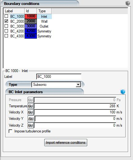
Subsonic inlets require the three velocity components and the static temperature. These values are imposed as Dirichlet conditions on all boundary nodes without the possibility to change them during iterations. You must check that the assigned velocity vector is in fact pointing into the computational domain at every node on the boundary, otherwise the calculations will diverge. button can be used to copy the velocity vector and the temperature from the initial/reference conditions specified in the Conditions tab.
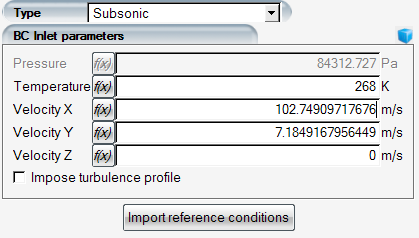
In subsonic inlets, the pressure is set free and cannot be adjusted while static temperature and velocity components are specified. The pressure of the domain will be set by the conditions on subsonic outlets.
This inlet boundary type is a more generic, which covers subsonic, supersonic, and far-field situations. In addition to static temperature and velocity, static pressure is also needed. The boundary automatically determines the inflow/outflow state of the boundary nodes using node normal vectors and the velocity direction to impose proper Dirichlet/free states for flow variables. In this manner, inflow nodes will act the same way as if they were set as subsonic, and outflow nodes will only impose pressure similar to a subsonic exit boundary. Clicking the button will copy all values from the Conditions panel.
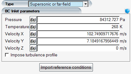
In the case of supersonic flow, all flow variables are imposed at the inflow nodes, and they are all set free on the outflow nodes.
Note: It is possible to have secondary subsonic inlets in supersonic flows (engine turbine exhausts before flow expansion) and supersonic inlets in subsonic flows (piccolo tube holes simulated as Mach = 1 inlets). The user should make sure that in the domain there are boundaries where pressure is set one way or another.
The stagnation inlet boundary is used to specify total pressure and temperature, along with the velocity direction. This boundary is suitable when the total conditions are known and the velocity is not available. The Import of reference conditions feature is not available for this subtype, therefore the button is disabled.
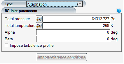
The current implementation of the stagnation inlet boundary condition is marginally stable and requires significantly lower CFL numbers. Engine inlet subtypes are recommended instead when the total pressure and temperature plus either the Mach number or the mass flow rate is known.
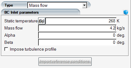
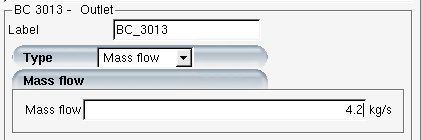
The mass flow inlet allows the specification of a mass flow rate with a given direction. Keep in mind that the area considered for the mass flow is the actual area of the boundary inlet as it appears in the grid, and not the full annular area, in case of rotationally periodic grids, or the full cross-section, in the case of symmetric grids. The static temperature also must be specified in a mass flow inlet.
The angles alpha and beta set the flow direction at the inlet. The ![]() icon can be clicked to visualize the flow direction that
will be imposed.
icon can be clicked to visualize the flow direction that
will be imposed.
The mass flow inlet is a subsonic boundary condition, and the pressure is set free like so. Therefore, in the domain, there must be an outlet boundary where the pressure is specified. You should pay attention to the value of the mass flow rate not to exceed sonic conditions at this boundary.
This is a non-reflective boundary condition based on 1D Riemann characteristics, and it is meant for far fields that are placed away from the solid. All five flow variables are provided, and they can float during the solution process.
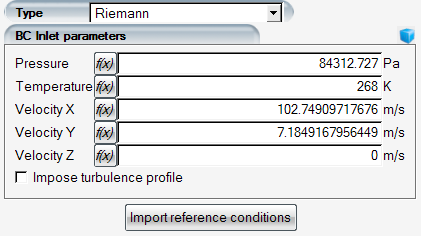
The purpose of this boundary condition is to provide better convergence for transonic flows and to allow some variation in the inflow velocity components when they are not known exactly. Use this inlet type if the far-field boundary condition has trouble converging or produces noise in the solution. Riemann boundary condition works better for high speed flows and may not converge as well for very low speed flows.
This is a variation of the stagnation inlet boundary condition that makes use of the 1D-Riemann formulation, and it can accept total temperature and total pressure with a ball-park mass flow rate. The alpha and beta angles are used to set the flow direction. All values can slightly float to adapt to the conditions that establish downstream of the inlet.
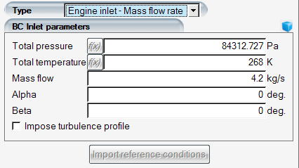
The engine inlet – mass flow boundary condition is best suited for turbomachine inflow boundaries, hot air sources like the inlets of ducts and piccolo tubes, etc. It converges significantly better compared to the stagnation inlet boundary condition.
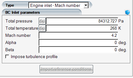
This is a variation of the condition, where instead of the mass flow rate the Mach number is specified.
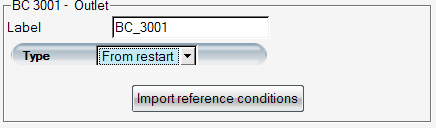
When an inlet boundary is set as From restart, it is treated as a supersonic or far-field boundary condition with the nodal values of all flow variables being assigned directly form the restart flow solution that was used to initialize the calculations. This is desirable in many occasions when the boundary conditions are not readily available or non-uniform and difficult to formulate.
Wall boundary indices range from 2,000 to 2,999. Wall indices ranging from 20 to 29 are still supported for backward compatibility, but are converted to the four-digit format. The surface type can be set to Slip for an inviscid flow (Euler equations), or to No-slip for a viscous flow (Navier-Stokes equations).
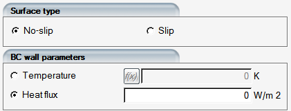
No-slip walls impose zero velocity on all nodes of the wall, unless the wall is rotating
No-slip walls in rotating frames get zero velocity relative to the frame, meaning they rotate with the frame. Turbomachine rotors, hubs, helicopter blades are examples. For static walls in rotational frames of reference like shrouds of turbomachinery rows, the Counter-rotating condition should be selected. It is possible to use slip walls in rotating frame, then the velocity on the surface will be tangent.
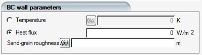
The thermal conditions on a no-slip wall are either temperature or heat flux specifications. For adiabatic walls, the heat flux should be set to 0.
Note: When the no-slip walls and the inlet intersect for internal flows, the nodes at the intersection will experience a large velocity gradient and therefore the results at these points may be noisy. To mitigate this noise, set the inlet type to Mass flow. This is a weak-form boundary type and permits a boundary layer velocity profile to form naturally.
Slip walls are used in inviscid flows in general, however there are times when they can be of use for viscous flows as well. In case of internal flow simulations where the inlet and exit boundaries might be too close to the region of interest, you should extend the inlet and exit passages via slip walls to prevent large flow variations and to provide uniform boundary conditions. The slip walls will not contribute to the boundary layer formation and the domain extensions will help obtain a smooth transition between the local and the boundary conditions.
Slip walls are not considered in the wall distance and y+ calculations in order not to interfere with the turbulence production/destruction terms of turbulence models.
The Sand-grain Roughness – BC type option is set in the Model → Roughness panel, as outlined in outlined in Variable Roughness from the Boundary Conditions, an additional box for the specification of the sand-grain roughness height on each wall surface will appear.
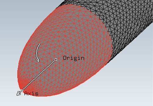
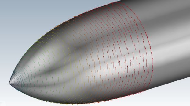
Rotating axisymmetric surfaces such as propeller spinners and engine nose cones can be simulated in steady-state computations by applying a tangential velocity at the grid nodes of the rotating surface. Given the rate of rotation, the components of the tangential velocity are automatically computed at each node of the surface according to its normal distance from the axis of rotation. This is useful if other non-rotating components are present, such as the engine nacelle, or even a complete aircraft, in which case the relative frame of reference could not be used.
Note: The rotating spinner must be a surface of revolution. The orientation of the axis of rotation of the spinner can be arbitrary, and it will be automatically detected by FENSAP-ICE.
To enable rotation for a (wall) surface, set Rotation to in the boundary conditions panel of the selected surface and specify the rotation rate in rpm. Click the button.
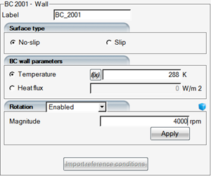
The axis of rotation of the selected surface is detected automatically and it is displayed in the 3D viewer panel for verification. The direction of rotation follows the right-hand rule convention. To reverse the direction of rotation, add a minus (-) sign in front of the magnitude of the rotation rate and click the button. This boundary condition can be applied to any number of spinners with any arbitrary orientation, even if the incoming flow is not parallel to their rotation axes.
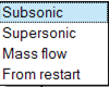
Outlet boundary indices range from 3,000 to 3,999. The indices 30 to 39 are supported for backward compatibility. There are four subtypes of outlet boundaries:
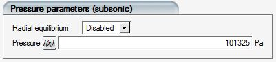
The subsonic outlet boundary condition specifies the pressure on the boundary nodes. In subsonic flows, these boundaries are the ones that set the final pressure for the whole domain since the only unchanging pressure values are found on subsonic outlets. By default the pressure is set as 101,325 Pa, and it is possible to set it to the reference pressure specified on the Conditions panel by clicking Import reference conditions.
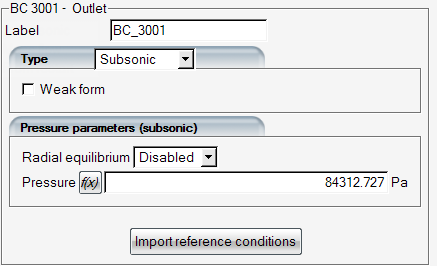
Normally the outlet boundary condition applies the pressure as a Dirichlet boundary condition. By turning on the Weak form option, the pressure can be applied as a contour integral instead. This permits the pressure values to locally float and partially adjust to the pressure variations reaching the outlets (wake of a rotor for example).
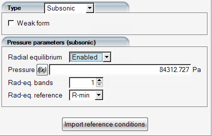
For subsonic exits with swirling flow, the radial equilibrium option is available to provide the necessary force balance between pressure and centrifugal forces that the fluid is experiencing. The outlet should be circular and flat, but can be oriented arbitrarily. The pressure set on the boundary can be specified at the largest or the smallest radius, depending on the case, using the Rad-eq. reference menu. Usually for turbomachinery exit boundaries it is convenient to set the hub as the reference pressure location. However, for external flows the perimeter of the exit boundary should be the reference point since this is where the far-field boundary with the same pressure would intersect.
The radial equilibrium formulation allows a piece-wise continuous implementation of the pressure gradient, helpful for cases where the angular velocity is non-uniform along the radius, especially in the case of external flows. The Rad-eq. bands setting allows you to set the number of bands to specify the piece-wise continuous distribution. Setting this to 1 means a standard linear distribution of dP/dr.
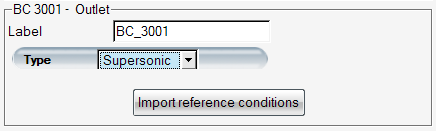
When the outlet is set as Supersonic, there is nothing to set and the pressure field at this location is free. The entire outlet boundary must be supersonic otherwise calculations can diverge.
The Mass flow outlet boundary condition takes a mass flow rate as the input for the entire boundary. This is a variation of the subsonic boundary where the uniform pressure is automatically adjusted until the desired mass flow rate is reached. The direction of the flow is dictated by upstream conditions as in the subsonic outlet case.
You should activate the Use variable relaxation option in the Solver panel, which ramps the CFL number from 1 to a target value using a specified number of iterations, when using this outlet boundary condition. This, in general, allows the pressure to settle more smoothly on the outlet boundary condition.
Mass flow outlet BC uses an under-relaxation factor of 0.1 by default which helps maintain stabile steady-state convergence for difficult problems. This is a global solver setting that applies to all mass flow outlet BCs and can be adjusted in the Solver – Advanced section. You can increase it up to 0.5 if you wish to converge the solution quicker.
If the mass flow rate specified is too high and choking conditions occur at the outlet, the target mass flow rate will be automatically lowered to keep the flow at Mach 1.
Note: Mass flow inlet and Mass flow exit boundary conditions cannot be used simultaneously if they are the only inlet and exit boundaries in the domain. This would make the pressure completely free and result in a non-unique solution. Somewhere in the domain, there must be a regular exit boundary condition with a specified pressure, or the inlet must be of Riemann or Engine Inlet type which will impose an external pressure to influence the free inlet pressure.
When From restart is selected for an outlet boundary condition, the pressure found on the restart solution is kept on the outlet nodes in Dirichlet form. This is useful when there is a restart file available with a non-uniform pressure distribution on the boundary (i.e. outlets of turbomachinery rows).
The Symmetry boundary condition can be used to reduce the mesh and domain size when the flow is perfectly symmetric across one or more planes. The boundary condition is applied through the use of pseudo elements also known as ghost cells that are exact copies of grid elements from the inner side of the symmetry plane, mirrored across the boundary. These elements serve to mimic the flow on the other side of the symmetry plane. They are included in the assembly of the finite element integrals on the symmetry planes, using vectors that are mirrored copies of the internal nodes. The new nodes on the pseudo elements are not included as degrees of freedom in the solution process, and they do not add to the solution time.
Traditionally 4000 – 4099 boundary conditions are of type General, 4100-4199 of type X-Symmetry, 4200-4299 of type Y-Symmetry, and 4300-4399 of type Z-symmetry, but with the introduction of the pseudo element technique all symmetry boundary conditions are treated in the same way. It is still important that individual symmetry boundary conditions are planar, and symmetry boundary conditions with different orientations should be numbered separately.
Note: FENSAP will not accept a curved symmetry boundary.
FENSAP-ICE supports both rotational and translational periodicity. The 5000 boundary family is designated for periodic boundaries, although this is only for CAD and flow visualization purposes. There are no boundary conditions imposed on periodic boundaries, instead, the implementation is similar to the symmetry boundary condition where grid elements from one (secondary) side are copied with translation or rotation to the other side (primary). The grid nodes on the primary side get full volume integrals for the FEM assembly as if a copy of the grid was there, without knowing about the periodicity condition. This ensures that the solution process is perfectly periodic.
Note: At the moment FENSAP-ICE requires that the periodic boundaries on either side are conformal, i.e. node to node matching.
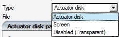
The 6000 boundary condition family is reserved for internal surfaces, which can be used as actuator disk for momentum sources, screens for momentum and particle sinks, heater pads in the case of solid conduction, or simply custom user set boundaries for flow visualization and quantity integration purposes.
The actuator disk model is a source term introduced directly in the surface integrals of the element faces lying on the disk to simulate rotor effects. To activate this model, select in the Type box.
The disk loading data is organized in (r,
 ) coordinates in a series of pressure loads and swirl velocity
distributions as a function of the radial coordinate ri
(1 ≤ i ≤ n) for an arbitrary number of constant angular
positions θj (1 ≤ j ≤ m).
The same number of radial coordinates ri
must be specified for each angular position θj, however the number (n) of radial coordinates ri
and number (m) of angular
positions θj may vary from disk to disk
when multiple disks are present.
) coordinates in a series of pressure loads and swirl velocity
distributions as a function of the radial coordinate ri
(1 ≤ i ≤ n) for an arbitrary number of constant angular
positions θj (1 ≤ j ≤ m).
The same number of radial coordinates ri
must be specified for each angular position θj, however the number (n) of radial coordinates ri
and number (m) of angular
positions θj may vary from disk to disk
when multiple disks are present.
Note: The total temperature source for the energy equation is calculated internally based on the total pressure sources.
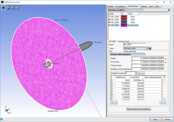
The boundary conditions can be imported from a user-supplied input file. To do so, click the disk icon and select the actuator disk boundary condition file. The format of this file is presented in The Actuator Disk File.
The actuator disk data can also be entered manually. A schematic illustration of the actuator disk is shown below:
The surface of the actuator disk may not necessarily be flat. In this case the loading data is specified on the pseudo-disk resulting from the projection of the actual disk on a flat surface perpendicular to the axis of rotation. FENSAP will take care of re-projecting the data back on the non-planar disk.
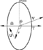
The vector  represents the fluid velocity as it passes through the
disk.
represents the fluid velocity as it passes through the
disk.
Note: The velocity through the disk is continuous, however it may not necessarily be perpendicular to the disk surface. The thrust will be applied in the specified thrust direction which does not have to be perpendicular to the disk, and the incoming flow may be at an angle to the disk.
The vector  denotes the unit vector perpendicular to the disk surface in
the general direction of the thrust generated by the disk. The vector
denotes the unit vector perpendicular to the disk surface in
the general direction of the thrust generated by the disk. The vector
 is the rotation axis which is used with the angular velocity
data provided in the disk file to calculate local tangential swirl velocity
components. The vector
is the rotation axis which is used with the angular velocity
data provided in the disk file to calculate local tangential swirl velocity
components. The vector  denotes the radial position on the disk, whose angular
position with respect to the 12 o'clock mark is
denotes the radial position on the disk, whose angular
position with respect to the 12 o'clock mark is  . Finally, the vector
  is the swirl velocity of the wake at that point.
Enter the geometry of the actuator disk:
Table 4.1: Actuator Disk Geometry
| Origin | The (X,Y,Z)-coordinates of the center of the disk |
| 12 o’clock | The (X,Y,Z)-coordinates of the 12 o'clock mark on the actuator disk's outer boundary |
| Thrust vector | The components of the thrust vector |
| Angular velocity | The components of the angular velocity vector, in rpm |
Click the display icon ![]() to display the center of the
actuator disk, the thrust vector and the 12 o’clock mark in the graphical
window. Click again to remove them from the graphical window.
to display the center of the
actuator disk, the thrust vector and the 12 o’clock mark in the graphical
window. Click again to remove them from the graphical window.
Note: The rotational velocity vector Ω follows the right-hand rule. The swirl velocity is not imposed as a Dirichlet boundary condition.
You should also set up the angular and radial distributions of disk loading and swirl velocity. Add a new radial distribution by clicking . The angular location should be given in degrees with respect to the 12 o'clock mark (coordinate in the direction of rotation; the orientation of the radial lines follows the right-hand rule with respect to the direction of the rotational velocity). Use the button to delete a selected radial distribution.
Enter the distribution of radial positions (Radius (m)), disk loading (Load (Pa)) and swirl velocities (Ang. Velocity (rad/s)) along this angular location. See The Actuator Disk File for the format of the actuator disk input file.
Important: The swirl velocity is not necessarily equal to the velocity of rotation of the actual rotor. The wake of a rotor rotates slower than the rotor itself, as induced by the drag at each blade section. The disk loading is the local force per unit area, and has the units of pressure (Pa).
The angular positions to for data specification must start at the 0˚ line and there should be at least four sectors defined in the disk data file. If the distribution is axisymmetric simply copy the same data to for the other sectors.
Data should not be provided at the 360˚ line, since it is identical to the 0˚ line.
User must ensure that the disk loading, integrated over the surface of the
actuator disk, produces the desired thrust. Similarly, the total enthalpy
jump ( ) integrated over the disk surface must yield the work done
on the fluid.
) integrated over the disk surface must yield the work done
on the fluid.
Use the two arrows  to expand or restrict the size of the table.
Effects of wire-mesh screens on air and droplet flows can be simulated using momentum resistance and mass loss coefficients across internal boundaries. A screen boundary introduces losses in air total pressure as well as liquid water content due to the blockage created by the wire mesh. To activate this model, the screen must be represented as an internal surface with a boundary index in the BC_6000 family in the grid file, similar to the convention shown in Actuator Disks. Mesh element on either side of this boundary must be connected, with no node duplication at the boundary. Unlike the circular actuator disk, the screen can be an internal surface of any shape. Select in the Type box of the screen surface.
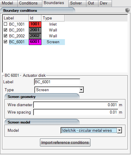
The generic screen geometry is described by a non-dimensional porosity
parameter  defined as:

where:
 - Wire diameter
 - Wire spacing
Presently, only screens with square mesh patterns can be simulated, however both planar and curved screens are supported.
Pressure drop across screens are usually described with the following formula:

Where  is the momentum resistance coefficient usually provided by an
empirical model,
is the momentum resistance coefficient usually provided by an
empirical model,  is the density of the fluid (in this case air), and
  is the flow speed. For 3D flows and where the flow is not
normal to the screen surface, the resistance applied to individual momentum
components will be different. This can be modeled with the following vector form
of the above definition:
is the flow speed. For 3D flows and where the flow is not
normal to the screen surface, the resistance applied to individual momentum
components will be different. This can be modeled with the following vector form
of the above definition:

In FENSAP, this vectorial form the of source term is applied in the momentum equations to simulate the effects of a screen placed at an arbitrary angle towards the flow.
A selection of momentum loss coefficient () models is available in the Screen model
section. They are described in the following sections.
The experimental correlation from Brundrett is as follows:


where  is the screen porosity as defined above, and
  is the wire diameter based on Reynolds number computed
locally around the screen using the normal flow component (therefore
incorporating cosθ in the original formulation) in FENSAP. This model
is reported to be valid for 1e-4 < Red <
1e4.
is the wire diameter based on Reynolds number computed
locally around the screen using the normal flow component (therefore
incorporating cosθ in the original formulation) in FENSAP. This model
is reported to be valid for 1e-4 < Red <
1e4.
The second model follows Diagram 8-1 in Idel'chik for a thin-walled grid of perforated sheets or strips with sharp-edged orifices: Idelchik, I.E., Handbook of Hydraulic Resistance, Second Edition, p. 402.

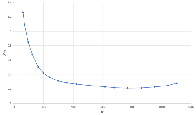
This model is based on Diagram 8-6 in Idel'chik for screens made of circular metal wires, with correction factors based on wire diameter:

where  is a coefficient to account for surface roughness of the
wires (default value 1.3), and
is a coefficient to account for surface roughness of the
wires (default value 1.3), and  is a wire Reynolds number-based correction factor obtained
from the following graph:
is a wire Reynolds number-based correction factor obtained
from the following graph:
The coefficient  is recommended to be 1.0 for brand new screens, and 1.3
for screens with nominal dust and wear. For other materials like silk
threads,
is recommended to be 1.0 for brand new screens, and 1.3
for screens with nominal dust and wear. For other materials like silk
threads,  was reported to be around 2.1. For iced screens, one could
justify using a much higher value to account for the roughness of ice.
Unfortunately, there are no recommendations available on this point at the
moment. This parameter is not available in the FENSAP-ICE UI, but can be
modified by adding
was reported to be around 2.1. For iced screens, one could
justify using a much higher value to account for the roughness of ice.
Unfortunately, there are no recommendations available on this point at the
moment. This parameter is not available in the FENSAP-ICE UI, but can be
modified by adding FSP_SCREEN_IDELCHIK_KZERO
value in a
user.par file located in the run directory.
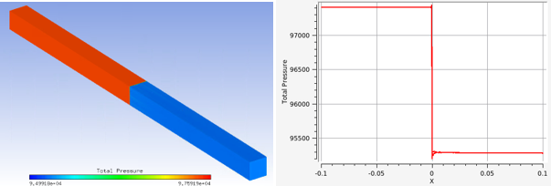
The following example shows the total pressure drop across a screen BC with 75% blockage. In this case, the air flows from left to right.
The 7000 boundary condition family is reserved for non-conformal interfaces in a domain. The interface pairing is detected as odd/even consecutive numbers, that is, 7001-7002 is a pair, 7005-7006 is a pair, and so on. Ansys file converters from ICEM CFD, CFX, or Fluent will be able to automatically assign these numbers, however, if the grid is created by a third-party method then you must pay attention to establish this odd/even pairing of interface boundaries. There are no settings to provide in the case of non-conformal interfaces.
The grid density on both sides of a non-conformal interface is recommended to be similar, especially if the edges of the interfaces are curved. Otherwise, the edge nodes of the finer side may physically reside outside of the elements of the coarser side and solution quality and convergence may be compromised as a result of poor interpolation between these two interfaces.
Ice displacement and mesh deformation do not support non-conformal interfaces, and nodes on these boundaries are static. Placing these interfaces close to icing walls is not recommended.
To ease data entry, the boundary conditions can be set by importing the reference conditions. For this, click Import reference conditions.
Note: The velocity components will not be set properly when starting a calculation from a previous solution (restart). In this case, the values should be entered manually.
The button indicates that the variable distribution is imposed through a function of the spatial coordinates.

For example, to impose a Velocity-X profile, click the button to open the formula window.
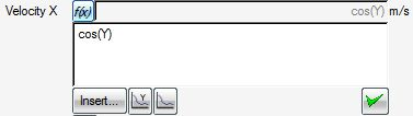
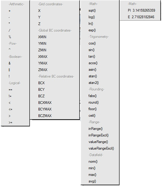
Enter a spatial distribution by using the button:

using the variables, functions and operators provided:
The equation can be a function of any combination of spatial coordinates, however it can only be displayed as 2D graphs in either X, Y or Z, selected with the buttons:

The other spatial coordinates are then set to zero to ease visualization.
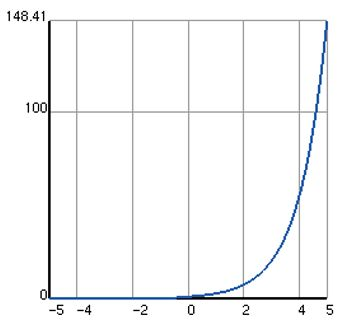
The following equation

can be entered as follows

The Boolean operator (X<=30) assumes a value of either 1 or 0 depending on whether the condition is true or false. The function f(x) is displayed in the graphical window for visual validation. Click the icon:

to refresh the display
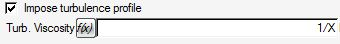
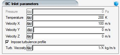
Any profile of the turbulent variables can be imposed at the inlet. To do so,
select Impose turbulence profile, click  and enter a profile for:
Turbulent viscosity (if using the Spalart-Allmaras one-equation model)
 and
and  (if using the
  -
-  two-equation models)
 and
and  (if using
  -
-  models)
Note: When this option is not activated, the uniform, constant turbulent variables values are automatically imposed on inlets from the input Eddy/laminar viscosity ratio set in the Model panel.