


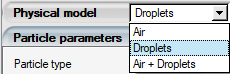
Select the option in the Physical model pull down menu of the Model panel to access the DROP3D configuration environment.
DROP3D solves the particle flow as a continuum, using the Eulerian formulation. The general Eulerian two-fluid model consists of the Euler or Navier-Stokes equations augmented by the particle (droplets or crystals) continuity and momentum equations:


Where the variables  and
and  are mean field values of, respectively, the particle concentration
and velocity. The first term on the right-hand-side of the momentum equation
represents the drag acting on particles of mean diameter
are mean field values of, respectively, the particle concentration
and velocity. The first term on the right-hand-side of the momentum equation
represents the drag acting on particles of mean diameter  . It is proportional to the relative particle velocity, its drag
coefficient
. It is proportional to the relative particle velocity, its drag
coefficient  and the droplets Reynolds number:

And an inertial parameter:

The second term represents buoyancy and gravity forces, and is proportional to the local Froude number:

These governing equations describe the same physical particle transport phenomena as current Lagrangian codes. Only the mathematical form in which these equations are derived changes, using Partial Differential Equations instead of Ordinary Differential Equations.
In addition to continuity and momentum conservation equations for particles, DROP3D can also solve the thermal energy transport equation. The particle thermal energy equation enables heat exchange between particles, air flow, and water vapor systems. For more details on the particle thermal equation formulation, consult The Particle Equations for more details.
Different particle types, and their related drag correlations, are supported by DROP3D.
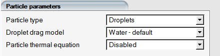
The Water - default drag coefficient is based on an empirical correlation for flow around spherical droplets, or:

The range of validity of this drag coefficient is not limited by the
 , but it is generally observed that water droplets start to deform
at values above
, but it is generally observed that water droplets start to deform
at values above  250.
250.
The second choice is based on Water - Stokes law for flow
around an isolated sphere. It is valid for very small  number (<1).

The third choice is an extended version of the default law, referred to here as
Water - extended Reynolds, defined with w = 
 as:
as:

The fourth drag coefficient correlation, Snowflakes, applies to oblate spheroids and is useful for calculating the collection efficiency of snowflakes:

With

The second Particle type model, Ice crystals, applies to oblate spheroids and computes the collection efficiency of ice crystals. The inertia parameter in this case is:

The common practice in evaluating the drag force is to assume that the particles
are spherical and rigid. This is indeed a valid approach for small water droplets,
but may not necessarily apply to ice crystals. Previous studies have shown that the
hydrodynamic behavior of a plate-like hexagon can be sufficiently approximated by
that of a circular disk. Pitter et al showed that a disk of a
finite aspect ratio  , where
  is the semi-major axis length and
  is the semi minor axis length, has properties similar to a thin
oblate spheroid at low to intermediate Reynolds numbers. The
drag coefficient is therefore calculated for a range of crystal
Reynolds numbers from the following correlations derived by
Pitter for crystals with aspect ratios
is the semi minor axis length, has properties similar to a thin
oblate spheroid at low to intermediate Reynolds numbers. The
drag coefficient is therefore calculated for a range of crystal
Reynolds numbers from the following correlations derived by
Pitter for crystals with aspect ratios  of about 0.05, but also works reasonably well for values up to
0.5.
of about 0.05, but also works reasonably well for values up to
0.5.


where the oblate spheroidal drag,  for low Reynolds numbers, formulated by
Happel and Brenner is:
for low Reynolds numbers, formulated by
Happel and Brenner is:

Mixed Particle Phase with

When both particle types (for example, droplets and crystals) are present, the inter-phase coupling for mass, momentum and energy transfer due to melting or freezing is handled within each individual system. Therefore both sets of dispersed-phase equations are treated in an uncoupled manner. If Particle Thermal Equation is not enabled, melting and evaporation are not modeled.
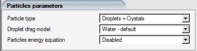
The Droplet drag model can be selected as in Particle Drag Correlations. The drag correlations of the ice crystals, outlined in Ice Crystal Drag Correlations, depend on the crystal type, which will be described in Appendix O - Supercooled Large Droplets.
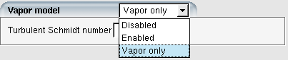
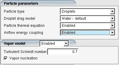
DROP3D can model vapor transport and simulate the mass and energy transfer between vapor and droplets/crystals. Select in the Vapor model option to activate this functionality. The Particle thermal equation under Particle parameters must be to allow the phase change. Besides the coupled mode, DROP3D can run vapor transport in a standalone mode. It can be activated by selecting Vapor only in the Vapor model. Droplet and crystal modeling will then be disabled.
The vapor transport equation can be written as follows:

where  and
and  are the vapor concentration and the air velocity, respectively.
 is a volumetric mass flux source or sink that represents vapor
condensation, droplet evaporation or crystal sublimation.
is a volumetric mass flux source or sink that represents vapor
condensation, droplet evaporation or crystal sublimation.  is the effective mass diffusion coefficient that combines laminar
and turbulent diffusion coefficients, for example,
is the effective mass diffusion coefficient that combines laminar
and turbulent diffusion coefficients, for example,  . The turbulent mass diffusion coefficient is computed by
 where
where  is the turbulent viscosity and
  is the turbulent Schmidt number. The default value of turbulent
Schmidt number is 0.7.
is the turbulent Schmidt number. The default value of turbulent
Schmidt number is 0.7.
Local water vapor pressure affects the rates of droplet and crystal evaporation, film evaporation at walls, and condensation onto walls and existing particles. Obtaining a valid solution for the humidity level and the vapor pressure is therefore important especially for engine icing simulations.
Model Description
The current version of the nucleation model simplifies the nucleation process by assuming that all vapor above saturation is immediately converted to liquid state in the form of nuclei. The model does not capture supersaturation. The rate of nucleation is calculated based on the resulting mass transfer rate between vapor concentration and nucleation solution fields, and is applied directly to the air flow energy equation as a source term. The numerical benefit of this assumption is the simplicity of the formulation which helps in creating a robust and reliable computational tool. Vapor and nuclei transport are modeled with the same species equation, avoiding additional computational cost.
Nuclei are tiny droplets with diameters in the order of a micron or less and assumed to move with the air velocity around objects at the scale of typical aircraft components. The nucleating mass is contained within the vapor transport system, and exchanged with vapor depending on local air temperature and humidity conditions. The release of enthalpy due to nucleation is exchanged with the air flow solution through a source term which calculates the rate of nucleation from the prescribed nuclei concentration in the volume.
When running vapor transport coupled with the air flow in FENSAP-ICE, an increase in air temperature will be observed where there is nucleation, and vice versa. If running DROP3D only with vapor transport enabled, this change in air temperature will not be captured and applied in the icing simulation. The removal of mass from the gas phase in the vapor transport equation will reduce local vapor pressure, vapor diffusion rate, and wall condensation, for regions where relative humidity was over 100%.
Activating Nucleation in Vapor Transport
The option to enable nucleation is found in the model panel of a run configuration window. It is listed under Vapor model:
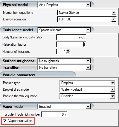
By default, this option is enabled when a new run is created. When enabled, there will be a new solution field in the vapor solution file called Nucleation (kg/m3), which shows the nuclei concentration in the computational domain. Together with the vapor concentration, the sum of the two quantities represent the total mass conserved with the vapor transport model. The relative humidity will be maximum 100% as any vapor over saturation is collected in liquid form in the nucleation field.
To observe the change in air temperature due to nucleation/evaporation within the vapor transport system,
Particle-Airflow thermal coupling (See Vapor, Air Particle Energy Coupling) should be used. It is possible to calculate air flow in energy only mode, following a restart with CFX or Fluent solution.
Note: Currently, the reduction in total pressure of air mixture due to nucleation is not modeled. This interaction will not be observed in the coupled vapor-air-particle-energy simulations. The convergence of the coupled air-vapor system may not be as monotonous as before since the energy coupling creates a feedback mechanism between air temperature, vapor saturation pressure, local humidity, and rate of nucleation. It may be required to reduce the CFL numbers for both systems if difficulty in convergence is observed.
Example 5.1: Solving a Coupled System of Air Flow, Crystals, and Vapor with Nucleation
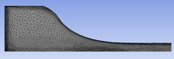
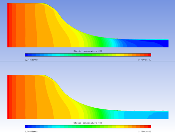
The example below solves a coupled system of air flow, crystals, and vapor with nucleation. The computational domain is a rotational periodic slice of a circular converging nozzle as shown in the figure below. The conditions on the inlet boundary which is at the left end of the domain are:
| Air properties | |
| Static temperature | 279.43 K |
| Speed | 2.85 m/s |
| Relative humidity | 80% |
| Crystal Properties | |
| Content | 1.07g/m3 |
| Diameter | 35 microns |
| Aspect ratio | 1 |
| Temperature | 250 K |
The only condition applied at the exit boundary to the right is the back pressure which is 42747.5 Pa.
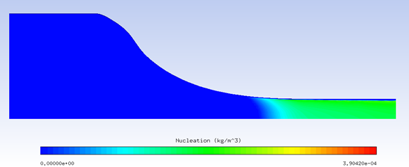
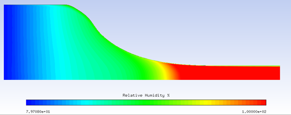
The high level of inflow humidity will suppress sublimation of crystals, and induce melting. The excess vapor will reach saturation as local static temperature drops due to air flow acceleration through the narrowing passage, and nucleation will happen. The figures below vapor nucleation, relative humidity, and air temperature with nucleation on and off. With the added heat of condensation of nuclei, air temperature increases several degrees.
Capturing Supersaturation
It is possible to capture supersaturation if droplets are substituted for nuclei and the standard diffusion based condensation acts to transfer mass from the vapor system onto the droplets. This would be done by setting the droplet size to a value presentative of aerosols (i.e. 0.04 microns), and the LWC to a very low value that would represent a realistic aerosol concentration (i.e. 50000/cm3).
Such a simulation will make use of 3 additional equations – droplet concentration, size, and energy – and will require significantly more number of iterations due to the high energy flux rates associated with such small size particles driving down the local time steps. Therefore the simplified nucleation model is currently offered as the default method.
Vapor solution fields include:
Vapor pressure (Pa)
Vapor concentration (kg/m3)
Nucleation (kg/m3)
Vapor condensation (kg/m2/s)
Relative humidity (%)
Wet-bulb temperature (K)
Mass-mixing ratio (g/kg)
Nucleation field contains the amount mass transported in the form of condensed water, separate from the droplet and crystal fields.
Vapor condensation field stores the rate of vapor deposition computed on walls when they are colder than the surrounding air, with a local saturation pressure lower than the surrounding vapor pressure.
Mass-mixing ratio is the ratio of water vapor in grams to dry air density in kilograms.
Starting with version 24R2, the vapor fields are saved in droplet and crystal solution files, except when running in vapor-only mode. This allows running particle size distributions with vapor enabled, and having the vapor fields combined in the final droplet or crystal combined solution files.
Evaporative heat fluxes cool droplets, resulting in droplets drawing energy from their surroundings and cooling the air around them by convection. Droplets can cool enough to change phase and become ice crystals. Similarly, ice crystals can heat up when introduced to warm air, partially or fully melt with local temperatures above the freezing point. Local vapor concentration strongly influences the rates at which these processes occur. Therefore, coupling the energy and mass exchange between droplets, crystals, vapor, and air is important when these systems are not introduced in a state of thermal equilibrium into the computational domain.
The energy coupling with air is modeled via the convective heat flux term between
particles and air. A volumetric heating term is included in the energy equation of
air. The conservative energy equation of air in terms of specific internal energy
 (J/kg) is

in which  is the viscous shear stress tensor and
  is the pressure. The last term
represents the volumetric heat loss rate per unit volume (W/m3), which represents the convective heat flux

The convective heat flux  also participates in the partial differential form of the particle
internal energy equation:
also participates in the partial differential form of the particle
internal energy equation:

in which  is the specific internal energy (J/kg) of a particle type
‘p’. The thermal exchange between airflow and particles is modeled
through the convective heat flux.
is the specific internal energy (J/kg) of a particle type
‘p’. The thermal exchange between airflow and particles is modeled
through the convective heat flux.
The evaporative heat flux in the above equation determines the mass to be exchanged with the vapor system. The change in heat is reflected onto the particle itself which can result in temperature or phase change.
Setup
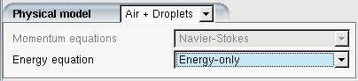
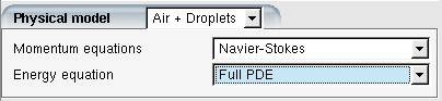
Create a DROP3D run under the working project and assign the air solution and grid as usual. In the Physical model, select the option in the pull-down menu of the Model panel. Normally the air-cooling effect due to thermal coupling has a negligible effect on the airflow’s momentum, therefore solving only the energy equation of air is enough. In most cases, choose for Energy equation. However, if you expect that the thermal coupling has a strong impact on the air’s motion, the option should be enabled.
Note: The water vapor partial pressure and density are not included in the bulk fluid properties with full coupling. At air static temperatures of 0 °C and 30 °C, the saturation vapor density is around 0.3% and 3.0% of bulk density, respectively. This is an indication of the error margin in the modeling process when pressure-momentum coupling of air and vapor is neglected.
In the Particle parameters panel, enable both Particle thermal equation and Airflow energy coupling. Enabling Vapor model is not mandatory to allow energy exchange between particles and the airflow. However, it is highly recommended to activate this model because the evaporation flux is tied to the local vapor pressure.
Important: If one wants to see the effect of thermal coupling on air temperature, it is very important to fully converge the initial air solution. This will ensure that changes in air temperature are entirely due to the thermal coupling, and not to convergence of the air system itself.
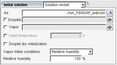
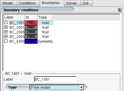
For the inlet and outlet airflow boundary conditions, select in the Type pull down menu to assign nodal values from the restart dry air solution. The droplet/crystal/vapor boundary conditions can be set as usual.
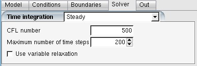
A CFL number is required for both airflow and particle solvers. In most cases,
where particle-airflow energy coupling is enabled, solving the air energy equation
is sufficient. If is selected for Energy
equation in the Model panel, the CFL
number can be increased up to 1000 or even
higher, depending on the problem at hand. If the option
is enabled instead, a CFL number used for regular airflow calculation can be
applied. The CFL number for droplet can stay at
20 or lower.
When preparing the air and particles solutions for an icing calculation, the walls should be kept adiabatic if vapor-air-particle energy coupling is active. Otherwise, the wall temperature setting will modify this energy balance and pollute the rest of the icing process. When adiabatic walls are used in air flow calculations, ICE3D runs should be done with EID option enabled, to obtain appropriate heat transfer coefficients.
For Multi-FENSAP simulations, the same setup described in this section can be followed to include two-way thermal coupling of particles and air in multi-shot icing simulations. The updated air solution files due to thermal coupling (soln.coupled.drop.######) will be used by the following ICE3D executions.