


Ansys Fluent allows you to control the appearance of the scene that is displayed in the graphics window. You can control the display state which consists of visual properties including the view, graphics effects and more. The view can be manipulated by scaling, centering, rotating, translating, or zooming the display. Display states can be saved, restored, copied and deleted (and the same applies to views). These operations are performed in the Display States Dialog Box (Figure 40.85: The Display States Dialog Box). For views, these operations are performed in the Views Dialog Box (Figure 40.87: The Views Dialog Box) or with the mouse, or simply using the shortcut in the graphics toolbar, as described in Selecting a View.
Important: You can revert to the previous view by pressing Ctrl+L while the graphics window
has the main focus. You can also use the text command view last from the top level of the text command tree.
You can use the command to revert to any of the past 20 views.
For additional information, see the following sections:
When you display a graphics object, you have the option of associating a display state with that object. The display state allows you to recreate the same display, both between multiple objects and across different sessions. You are not required to associate a state with an object, nor do you have to preserve every aspect of a particular display. The following fields can be included in a display state:
View
Front Faces Transparent
Projection
Axes
Ruler
Boundary Markers
Titles
Light ID
Note: When you click Use Active, either in the Display States dialog box or from within a graphics object dialog box, the behavior depends on how many light IDs are active:
If only one light ID is active then that light ID is populated in the Light ID field.
If more than one light ID is active then the Light ID field is set to Don't Save.
Headlight
Lighting
Anti-Aliasing
Reflections
Static Shadows
Dynamic Shadows
Grid Plane
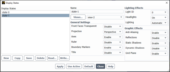
In many cases, you should not have to use the Display States dialog box, because you can setup the window and object(s) as desired, then right-click in the graphics window and select Save State. If you still have the dialog box for the graphics object open, for example the Contours dialog box, you can click Use Active to create a display state that matches that of the active graphics window and click to associate that display state with the object. Alternatively, you can select a pre-existing display state from the drop-down list, which can allow you to create multiple objects that will display with a consistent orientation and appearance.
Important: Display state settings (except the view) are applied to all user (non-2D plot) windows.
For example, if you display a contour plot with a display state that includes the ruler, then display a vector plot in a new window with a display state where the ruler is disabled, the ruler will be disabled in both plot windows.
Note: Graphics object that are displayed with None selected as the Display State will be shown with the same display state settings as the last displayed object.
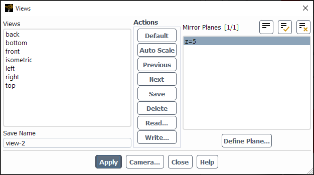
You can use the Views Dialog Box (Figure 40.87: The Views Dialog Box) to select the orientation of your
display or use the ![]() drop-down available in the graphics toolbar for
3D simulations. Furthermore, you can simply click the interactive
triad (Figure 40.86: Using the Triad to Change the Orientation of the Object), displayed in the graphics
window. The Table 40.1: Standard Views relates the Views listed in the Views Dialog Box to the views available
in the graphics toolbar (see Pointer Tools).
drop-down available in the graphics toolbar for
3D simulations. Furthermore, you can simply click the interactive
triad (Figure 40.86: Using the Triad to Change the Orientation of the Object), displayed in the graphics
window. The Table 40.1: Standard Views relates the Views listed in the Views Dialog Box to the views available
in the graphics toolbar (see Pointer Tools).
![]() Results → Graphics
Results → Graphics ![]() Views...
Views...
Table 40.1: Standard Views
|
View Listed in Dialog Box |
View Shortcut in Graphics Toolbar |
|---|---|
|
back |
|
|
bottom |
|
|
front |
|
|
isometric |
|
|
left |
|
|
right |
|
|
top |
|

To change the orientation of the object in the graphics window using the triad (Figure 40.86: Using the Triad to Change the Orientation of the Object), you can
Click an axis/semi-sphere to point it in the positive/negative direction.
Right-click an axis/semi-sphere to point it in the negative/positive direction.
Click the cyan iso-ball to set the isometric view.
Click the white rotational arrows at the bottom of the triad to perform in-plane clockwise or counterclockwise 90 degree rotations.
Left-click and hold—in the vicinity of the triad—and use the mouse to perform free-rotations in any direction. Release left mouse button to stop rotating.
Note that clicking on the X-axis will result in the +X-axis pointing towards you.
Note: For 2D cases, the ![]() drop-down and the interactive triad are not available; in a
front view, the X-axis is horizontal with the positive direction to the right,
the Y-axis is vertical with the positive direction pointing up, and the Z-axis
is determined by the right-hand rule.
drop-down and the interactive triad are not available; in a
front view, the X-axis is horizontal with the positive direction to the right,
the Y-axis is vertical with the positive direction pointing up, and the Z-axis
is determined by the right-hand rule.
Most of the manipulating activities (like scaling and centering the display) are accomplished using the Views Dialog Box (Figure 40.87: The Views Dialog Box).
![]() Results → Graphics
Results → Graphics ![]() Views...
Views...
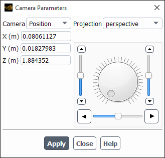
You can rotate, translate, and zoom the graphics display using either the mouse or the Camera Parameters Dialog Box (Figure 40.88: The Camera Parameters Dialog Box), which is opened from the Views Dialog Box.
You can scale and center the current display without changing its orientation by clicking in the Views Dialog Box.
Use either the mouse or the Camera Parameters Dialog Box to:
Rotate the display in any direction (in 3D)
Rotate the display about the axis normal to the screen (in 2D)
To rotate a display with the mouse, use the button with the Rotate (Pan in 2D) function (the left button, by default). For information about changing the mouse functions, see Controlling the Mouse Button Functions.
Click and drag the left mouse button in the graphics window to rotate the geometry in the display.
You can also click and drag the left mouse button on the (
 ,
,  ,
,  ) graphics triad in the lower left corner to rotate the
display.
) graphics triad in the lower left corner to rotate the
display.If you press the Shift key when you first click the mouse button to begin the rotation, the rotation will be constrained to a single direction (for example, you can rotate about the screen’s horizontal axis without changing the position relative to the vertical axis).
If you want to constrain the rotation of a display to be about the axis normal to the screen, you can also use the Roll-Zoom function.
Click the appropriate mouse button and drag the mouse to the left for clockwise rotation, or to the right for counterclockwise rotation.
To rotate a 3D display using the Camera Parameters Dialog Box (Figure 40.88: The Camera Parameters Dialog Box) use the dial and the slider of the scales.
To rotate about the horizontal axis at the center of the screen, move the slider on the scale to the left of the dial up or down (see Scales or instructions on using the scale).
To rotate about the vertical axis at the center of the screen, move the slider on the scale below the dial to the left or right.
To rotate about the axis at the center of and perpendicular to the screen, click the left mouse button on the indicator in the dial and drag it around the dial.
Important: The position of the slider or the dial indicator does not reflect the cumulative rotation about the axis as the slider/indicator will return to its original position when you release the mouse button.
When you use the mouse for rotation, you have the option to
“push” the display into a continuous spin. This feature
can be used in conjunction with video recording, or simply for interactive
viewing of the domain from different angles. To use this option, use
the auto-spin? text command:
display → set → rendering-options → auto-spin?
Then display the graphics (or, if the graphics are already displayed, you can click in the Display Options Dialog Box). The Rotate (Pan in 2D) button will then have two uses:
To perform the standard rotation, stop dragging the mouse before you release the Rotate (Pan in 2D) button.
To start the continuous spin, release the Rotate (Pan in 2D) button while you are still dragging the mouse. The display will continue to rotate on its own until you click any mouse button in the graphics window again. The speed of the rotation will depend on how fast you are dragging the mouse when you release the button.
For smoother rotation, enable the Double Buffering option in the Display Options Dialog Box (see Modifying the Rendering Options). This will reduce screen flicker during graphics updates.
By default the left mouse button is set to Pan in 2D. For information about changing the mouse functions, see Controlling the Mouse Button Functions. Click and drag the left mouse button in the graphics window to translate the geometry in the display.
In 3D, you can either change one of the button functions to Pan and follow the instructions above for 2D, or use the Zoom button (the middle button by default). Click the middle button once on the point in the display that you want moved to the center of the screen. Ansys Fluent will redisplay the graphic with that point in the center of the window. This method can also be used in 2D.
In both 2D and 3D you will use the mouse button with the Zoom function (the middle button by default) or the Roll-Zoom function (see Controlling the Mouse Button Functions for information about enabling this optional function), or the Camera Parameters Dialog Box to magnify and shrink the display.
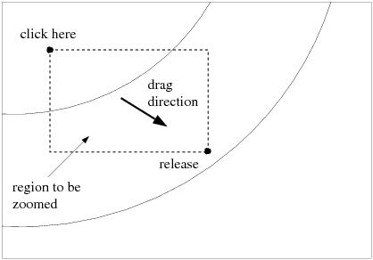
With the Zoom function, click the middle mouse button and drag it from left to right (creating a "zoom box") to magnify the display. Figure 40.89: Zooming In (Magnifying the Display) displays the correct dragging of the mouse, from upper left to lower right on the display, in order to zoom. You can also drag from lower left to upper right. After you release the mouse button, Ansys Fluent will redisplay the graphic, filling the graphics window with the portion of the display that previously occupied the zoom box.
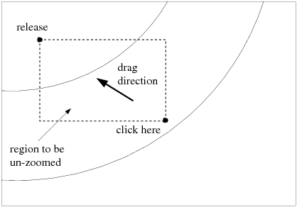
Click the middle mouse button and drag it from right to left to shrink the display. Figure 40.90: Zooming Out (Shrinking the Display) displays the correct dragging of the mouse, from lower right to upper left on the display, in order to "zoom out". You can also drag from upper right to lower left. After you release the mouse button, Ansys Fluent will redisplay the graphic, shrinking the graphical display by the ratio of sizes of the zoom box you created and the previous display.
With the Roll-Zoom function, click the appropriate mouse button and drag the mouse down to zoom in continuously, or up to zoom out. In the Camera Parameters Dialog Box (Figure 40.88: The Camera Parameters Dialog Box), use the scale to the right of the dial to zoom the display. Move the slider bar up to zoom in and down to zoom out.
Important: If you want to zoom in or out while the solver is iterating, click ![]() to assign Zoom In/Out to the
left-mouse-button prior to beginning the calculation. Roll zoom,
using the middle scroll wheel, does not work while the solver is
running.
to assign Zoom In/Out to the
left-mouse-button prior to beginning the calculation. Roll zoom,
using the middle scroll wheel, does not work while the solver is
running.
Perspective and other camera parameters are defined in the Views Dialog Box, which you can open by clicking Camera... in the Camera Parameters Dialog Box (Figure 40.87: The Views Dialog Box).
![]() Results → Graphics
Results → Graphics ![]() Views...
Views...
You may choose to display either an orthographic view or a perspective view of your graphics. To show a perspective view (the default), select Perspective in the Projection drop-down list in the Views Dialog Box (Figure 40.88: The Camera Parameters Dialog Box). To turn off perspective, select Orthographic in the Projection drop-down list.
Instead of translating, rotating, and zooming the display as described in Manipulating the Display, you may sometimes want to modify the “camera” through which you are viewing the graphics display.
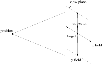
The camera is defined by four parameters: position, target, up vector, and field, as illustrated in Figure 40.91: Camera Definition. "Position" is the camera’s location. "Target" is the location of the point the camera is looking at, and "up vector" indicates to the camera which way is up. "Field" indicates the field of view (width and height) of the display.
To modify the camera’s position, select Position in the Camera drop-down list and specify the X, Y, and Z coordinates of the desired point. To modify the target location, select Target in the Camera drop-down list and specify the coordinates of the desired point. Select Up Vector to change the up direction. The up vector is the vector from (0,0,0) to the specified (X,Y,Z) point. Finally, to change the field of view, select Field in the Camera list and enter the X (horizontal) and Y (vertical) field distances.
Important: Click after you change each camera parameter (Position, Target, Up Vector, and Field).
After you make changes to the view shown in your graphics window, you may want to save the view so that you can return to it later. Several default views are predefined for you, and can be easily restored. All saving and restoring functions are performed with the Views Dialog Box (Figure 40.87: The Views Dialog Box).
![]() Results → Graphics
Results → Graphics ![]() Views...
Views...
Important: Note that settings for mirroring and periodic repeats are not saved in a view.
When experimenting with different view manipulation techniques, you may accidentally "lose" your geometry in the display. You can easily return to the default (front) view by clicking in the Views Dialog Box.
After manipulating the display and viewing it from different angles, you can return to previous displays by clicking in the Views Dialog Box.
Once you have created a new view that you want to save for future use, enter a name for it in the Save Name field in the Views Dialog Box and click . Your new view will be added to the list of Views, and you can restore it later as described below.
If a view with the same name already exists, you will be asked in a Question Dialog Box if it is OK to overwrite the existing view. If you overwrite one of the default views (top, left, right, front, and so on), be sure to save it in a view file if you want to use it in a later session. Although all views are saved to the case file, the default views are recomputed automatically when a case file is read in. Any custom view with the same name as a default view will be overwritten at that time.
As mentioned previously, all defined views will be saved in the case file when you write one. If you plan to use your views with another case file, you can write a “view file” containing just the views. You can read this view file into another Fluent session involving a different case file and restore any of the defined views, as described below.
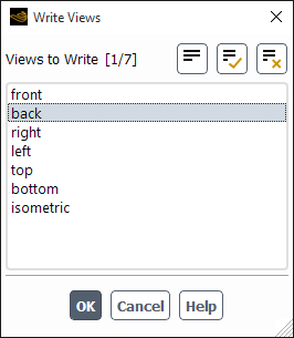
To save a view file, click in the Views Dialog Box. In the resulting Write Views Dialog Box (Figure 40.92: The Write Views Dialog Box), select the views you want to save in the Views to Write list and click . You will then use the Select File dialog box to specify the file name and save the view file. See The Select File Dialog Box for more details.
If you have saved views to a view file (as described above), you can read them into your current Fluent session by clicking Read... in the Views Dialog Box, and indicating the name of the view file in The Select File Dialog Box. If a view that you read has the same name as a view that already exists, you will be asked in a Question Dialog Box if it is OK to overwrite (that is, replace) the existing view.
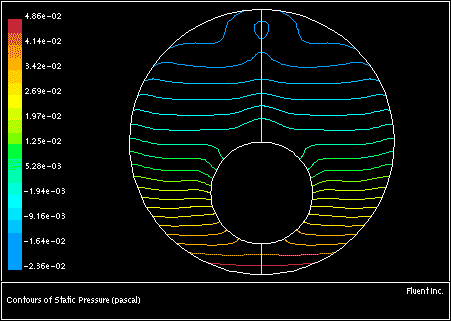
If you model the problem domain as a subset of the complete geometry using symmetry or periodic boundaries, you can display results on the complete geometry by mirroring or repeating the domain. For example, only one half of the annulus shown in Figure 40.93: Mirroring Across a Symmetry Boundary was modeled, but the graphics are displayed on both halves. You can also define mirror planes or periodic repeats just for graphical display, even if you did not model your problem using symmetry or periodic boundaries.
Display of periodic repeats is accessed directly in the View ribbon tab, while display of symmetries is accessed from the Views Dialog Box (Figure 40.95: The Views Dialog Box), which is also available in the View ribbon tab.
![]() View → Display →
Periodic Instancing...
View → Display →
Periodic Instancing...
![]() View → Display
→ Views...
View → Display
→ Views...
For a symmetric domain, all symmetry boundaries are listed in the Mirror Planes list. Select one or more of these boundaries as the plane(s) about which to mirror the display.
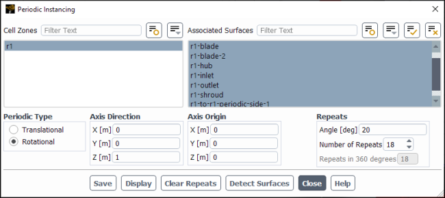
For a periodic domain, click Periodic Instancing... to open the Periodic Instancing Dialog Box, to access the periodicity parameters. Specify the number of times to repeat the modeled portion by increasing the value of Number of Repeats. If, for example, you modeled a 90° sector of a duct and you wanted to display results on the entire duct, you would set Number of Repeats to 4.
In some cases, there may be multiple zones with different periodicity in the domain. For example, in turbomachinery problems with multiple blade rows using the mixing plane model, the periodic angles are different for each blade row. One blade may contain 20 blades (18° periodic angle) and other may contain 15 blades (24° periodic angle). In such cases select the required cell zone and specify the number of repeats for that particular cell zone.
When you click Display in the Periodic Instancing Dialog Box the graphics display will be immediately updated to show the requested periodic repeats (assuming the periodic zones are displayed, either as mesh or as another representative graphics object).
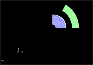
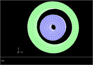
Figure 40.96: Before Applying Periodicity and Figure 40.97: After Applying Periodicity shows the display for the
sample geometry before and after applying the periodic repeats respectively.
In this case the value of Number of Repeats is
set to 6 for the 60° sector (outer part)
and to a value of 4 is set for the 90°
sector (inner part) of the geometry.
To define graphical periodicity for a non-periodic domain, do the following:
Click in the View ribbon tab (Display group box) to open Figure 40.98: The Periodic Instancing Dialog Box.
(Optional) Click to have Fluent automatically assess the case file and select what it thinks are the appropriate cell zones, surfaces, and other settings (such as angle and number of repeats) for this problem, and saves them.
Assuming Fluent correctly identifies the expected periodics, you can proceed with clicking , since the periodic instancing setup is now complete (assuming the periodic zones are displayed, either as mesh or as another representative graphics object).
Select the Cell Zone you want repeated.
Select Associated Surfaces that you want repeated.
Specify Rotational or Translational as the Periodic Type.
For translational periodicity, specify the Translation distance of the repeated domain in the X, Y, and Z directions. For rotational periodicity, specify the axis about which the periodicity is defined and the Angle by which the domain is rotated to create the periodic repeat. For 3D problems, the axis of rotation is the vector passing through the specified Axis Origin and parallel to the vector from (0,0,0) to the (X,Y,Z) point specified under Axis Direction. For 2D problems, you will specify only the Axis Origin; the axis of rotation is the
 -direction vector passing through the specified point.
Specify the Number of Repeats for the selected cell zone. Note that specifying a negative number will repeat the selected zone in the opposite direction.
Click .
Follow the same procedure for other cell zones.
Click in the Views Dialog Box to visualize the modified display.
You can clear any periodicities you have defined for the graphics by clicking .
Note:
For the 3D domain with multiple periodic zones having different periodicity, Ansys Fluent can repeat only mesh, contour and vector plots, and not the pathlines and particle tracks. Also if such domain contains, iso-surfaces and clip-surfaces, that are associated with a particular cell zone, they are repeated using the same periodicity that is defined for that cell zone. However, if the surface is not associated with any cell zone, you cannot specify the periodicity for that surface.
If you have an iso-surface that traverses multiple fluid zones, then this iso-surface will not be included in the surface detection (initiated via ). The proper way of taking advantage of the periodic instancing feature is to create an independent iso-surface cut within each fluid zone.
Transparencies assigned to the graphics display using the Scene dialog box are not applied to the repeat surfaces.
To define a mirror plane for a non-symmetric domain, do the following:
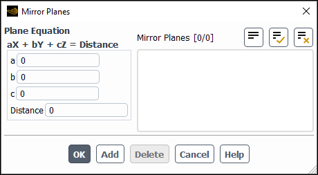
Click under Mirror Planes in the Views Dialog Box.
In the resulting Mirror Planes Dialog Box (Figure 40.99: The Mirror Planes Dialog Box), set the coefficients a, b, c, and the Distance (of the plane from the origin) in the following equation for the mirror plane:

(40–1)
Click to add the defined plane to the Mirror Planes list. When you are done creating mirror planes, click . The newly defined plane(s) will now appear in the Mirror Planes list in the Views Dialog Box. To include the mirroring in the display, select the plane(s) and click , as described above.
If you want to delete a mirror plane that you have defined, select it in the Mirror Planes list in the Mirror Planes Dialog Box and click Delete. When you click in this dialog box, the deleted plane will be removed permanently from the Mirror Planes list in the Views Dialog Box.