This section describes the process for loading the adjoint solver module, as well as setting up, running, and postprocessing the adjoint solutions. This section also demonstrates how the adjoint solution can guide the modification of the boundary shapes or turbulence model parameters.
The typical use of the adjoint solver involves the following steps (though not all of these may be necessary for every workflow):
Load or compute a conventional flow solution.
Specify the observable(s) of interest.
Set the adjoint solver controls.
Set the adjoint solver monitors and convergence criteria.
Initialize the adjoint solution and iterate to convergence.
For shape optimization:
Postprocess the adjoint solution to extract the sensitivity of the observable with respect to the boundary condition settings and the shape of the geometry.
Set up the Design Tool and calculate the optimal design change.
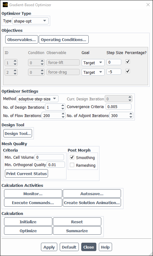
Modify the boundary shapes based on shape-sensitivity data and recompute the flow solution. The former can be done through the Design Tool, whereas multiple iterations of both the former and the latter can be performed by the Gradient-Based Optimizer.
For turbulence model optimization:
Postprocess the adjoint solution to extract the sensitivity of the observable with respect to the turbulence model settings and the shape of the geometry.
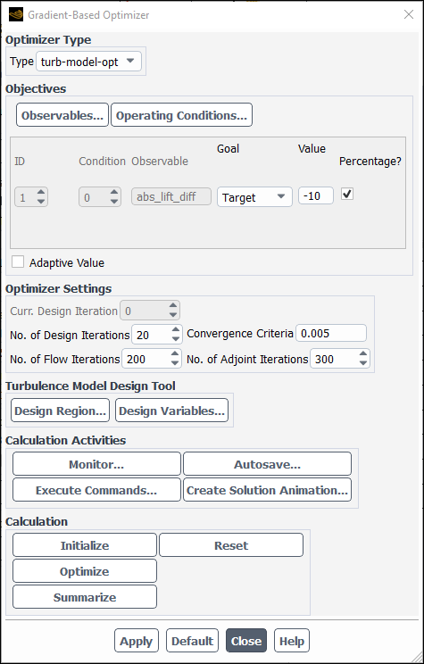
Use the Gradient-Based Optimizer and Turbulence Model Design Tool to modify the turbulence model parameters based on flow-sensitivity data and construct an augmented turbulence model.
This section provides information about using the Ansys Fluent adjoint solver in the following sections:
In addition, see the Fluent Tutorials for more information about using the adjoint solver. (To access tutorials and their input files, go to the tutorials area of the customer site.)
The current adjoint solver implementation provides basic adjoint solutions that accompany a conventionally-computed flow solution provided certain criteria are met.
The adjoint solver is implemented on the following basis:
The flow state is for a steady single-phase flow, or ideal gas, that is either laminar or turbulent.
For turbulent flows, the k-ε and k-ω models are supported. When the adjoint turbulence equation is not enabled, a frozen turbulence assumption is made, in which the effect of changes to the state of the turbulence is not taken into account when computing sensitivities. When the adjoint turbulence equation is enabled with the GEKO turbulence model, the effect of changes to the state of the turbulence will be taken into account when computing sensitivities.
The adjoint solver supports both user-defined scalar (UDS) and species transport equations, up to 50 adjoint UDS/adjoint species equations can be specified. When the adjoint UDS/adjoint species equations are not enabled, a frozen UDS/frozen species assumption is made, where the effect of changes to the state of the UDS/species are not taken into account when computing sensitivities. When the adjoint UDS/adjoint species equations are enabled, the effect of changes to the state of the UDS/species will be taken into account when computing sensitivities.
Adjoint species is supported for the following species models and species settings:
Species Transport model
Chemistry Solver
None - Direct Source
Stiff Chemistry Solver
Volumetric reactions
Diffusion Energy Source species transport options
All Turbulence-Chemistry Interaction options.
For details on these settings see Species Model Dialog Box.
The adjoint solver does not support 2d axisymmetric cases.
For moving (that is, non-inertial) reference frame problems, the single reference frame (SRF) and multiple reference frame (MRF) approaches are supported (as long as the absolute velocity formulation is used), while the mixing plane model (MPM) is not. Note that for the MRF approach, the adjoint solver does not support having a zone with a frame of motion that is relative to an already moving reference frame.
Solid zones are supported, as long as they do not use a moving reference frame approach.
By default, the adjoint solver uses spatial discretization methods that are chosen for stability. If desired, you can select more accurate methods, as described in Using the Adjoint Solution Methods Dialog Box.
The adjoint solver supports constant values for all material properties; non-constant functions are only supported for the following. If you are using a non-constant function not included in this list, the sensitivity accuracy may be reduced; even so, for most cases the sensitivity results will still provide useful information.
Density :
ideal-gas
incompressible-ideal-gas
piecewise-linear
piecewise-polynomial
polynomial
expression (as a function of temperature only)
Cp (Specific Heat) :
piecewise-linear
piecewise-polynomial
polynomial
nasa-9-piecewise-polynomial
kinetic-theory
Thermal Conductivity :
piecewise-linear
piecewise-polynomial
polynomial
expression (as a function of temperature only)
kinetic-theory
Viscosity
piecewise-linear
piecewise-polynomial
polynomial
expression
power-law
sutherland
kinetic-theory
Mass Diffusivity
constant-dilute-appx
dilute-approx
unity-lewis-number
UDS Diffusivity
polynomial
expression (as a function of temperature or pressure)
The boundary conditions are only of the following types:
Wall boundaries are supported with the following limitations:
Thin walls and shells are not supported.
Only Heat Flux, Temperature, and via System Coupling are supported for Thermal walls.
Only No Slip is supported for the Shear Condition.
Velocity inlet
Mass-flow inlet
Mass-flow outlet
Pressure inlet
Pressure outlet
Note that the Prevent Reverse Flow option is not considered in the adjoint calculation.
Pressure far-field
Symmetry
Rotational and translation periodic
Most of the boundary conditions in the above list can be defined using profiles, however, ensure that there are no warnings as described below upon initializing the adjoint solver.
Constant and user-defined sources defined by either an expression or UDF are supported for the momentum equation and for scalar transport equations such as the energy equation, turbulence equations, and UDS/species transport equations. See User-Defined Sources for details.
It is important to note that these requirements are not strict conditions for the conventional flow solver, but rather modeling limitations for the adjoint solver.
When the adjoint solver is initialized or an observable is evaluated, and before iterations are performed, a series of checks is performed to determine the suitability of the existing flow solution for analysis with the adjoint solver. Two types of message may appear:
Warning message: There are certain physics models and boundary condition types that are not explicitly modeled in the adjoint solver, but their absence does not disallow you from proceeding with the calculation. In this case, a warning message will be printed that explains the nature of the inconsistency.
Checking adjoint setup...
 -- Warning: Model is active but not included in adjoint calculation: P1 radiation model Done
The adjoint solver will still run in this case but the quality of the adjoint solution data can be expected to be poorer as a result of the inconsistency. This is because in such cases the unsupported settings will revert to corresponding supported settings for the adjoint solver. Though the calculation will proceed, it is important to note that the results produced should be considered on this basis. When reverting back to the fluid calculation, the original settings will be preserved and the modified settings are not migrated onto the original case. The warning indicates that the setting change will be made automatically and specifically for the adjoint solution.
Error message: There are some model and boundary conditions that are incompatible with the computation of an adjoint solution with the current adjoint solver implementation. In this case, an explanatory error message will be printed in the console window.
Checking adjoint setup...
 ** Unable to proceed: Model is active but not compatible with adjoint calculation:
  Transition SST turbulence model
Done
The adjoint solver will not run in this case and changes must be made manually to the settings identified in the console before the solver can be run.
User-defined sources can be created for the momentum equation or for scalar
transport equations such as the energy equation, turbulence equations, species
transport equations, and user-defined scalar (UDS) transport equations.
User-defined sources that are defined in compiled UDFs can be accounted for in
the application of the adjoint solver, provided that the source derivatives with
respect to flow variables and cell centroid coordinates are provided. This is
achieved by creating the source term UDF definition in the usual fashion, with
the exception that a special UDF macro is used,
DEFINE_SOURCE_AE (The suffix
_AE denotes Adjoint Enabled).
DEFINE_SOURCE_AE (name ,
c, t ,
dS, eqn)
|
Argument Type |
Description |
|---|---|
|
|
UDF name |
|
|
Index that identifies cell on which the source term is to be applied |
|
|
Pointer to cell thread |
|
|
Array that contains the derivative of the source term with respect to the dependent variable of the transport equation, as well as the flow variables and cell centroid position |
|
|
Equation number |
Function returns
real
Consider a source that may depend on velocity, pressure, cell-centroid coordinates, temperature, tke coefficient, omega equation, uds equations, and species equations:
Where,
,
, and
are the Cartesian velocity components in the cell.
is the pressure in the cell.
are the cell centroid coordinates as defined by the
C_CENTROIDmacro.is the temperature in the cell.
is the value of the turbulence kinetic energy in the cell.
is the specific dissipation rate in the cell.
is the (n)th user defined scalar in the cell.
is the (n)th species mass fraction in the cell.
If the source strength depends on one or more of these quantities, then the
derivatives of the source strength with respect to those variables must be
computed and filled in as entries to the dS[] array. In
particular,
|
|
|
|
|
|
|
|
|
|
|
|
|
|
must be defined in the UDF if there is a dependency of the source upon them. The specification of this derivative information is essential for sensitivities, including shape sensitivity, to be computed correctly by the adjoint solver.
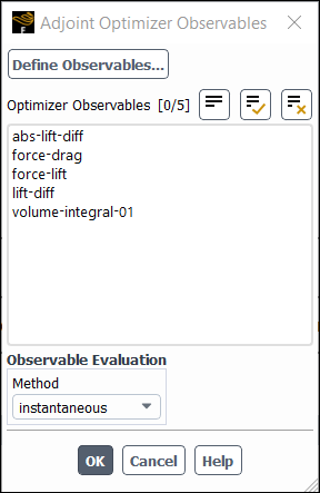
Defining an observable is a key initial step that must be performed for any adjoint calculation. The observable is the quantity for which sensitivities are sought. Observables can be defined based on flow variables, or as operations on other observables. For a list of the types of observables you can define refer to General Observables and General Operations. You can define multiple observables, but only one observable at a time can be selected for the adjoint sensitivity calculation.
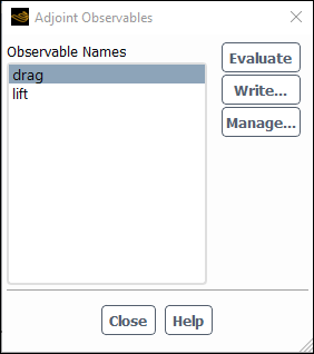
Observables are created and selected in the Adjoint Observables dialog box, which is accessed by clicking in the Design ribbon tab (Gradient-Based group box). (Figure 48.1: Adjoint Observables Dialog Box).
Design →
Gradient-Based →
Observable...
For more information, see the following sections:
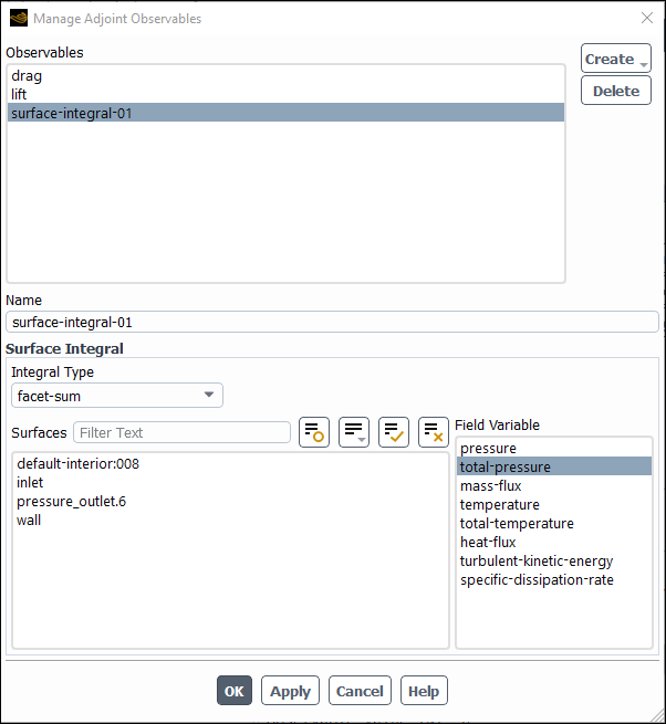
You can create a new observable by defining a single valued expession or by clicking Manage... in the Adjoint Observables dialog box and then Create... in the Manage Adjoint Observables dialog box.
From the Create... drop-down list you can choose from several observable types and operation types. Various types of observable quantities can be defined and the available types of observables are described in General Observables.
From the Observable types drop-down you can pick an observable from the list. Similarly, you can select an operation from the Operation types drop-down list. You can also select an observable to combine existing observables in various ways or apply unary operations to create a wide variety of compound observables. The operations that you can apply to existing observables are described in General Operations.
Once selected, you must edit the definition of the new observable within the Manage Adjoint Observables dialog box( Editing Observable Definitions).
Once an observable is created, it appears in the Observables list. When you select an observable in the Observables list, the Manage Adjoint Observables dialog box changes to expose various properties that can be assigned for the selected observable.
Once the observable properties are defined (Inputs for Observable Types), click Apply to apply the settings and proceed to define other observables, or click in the Manage Adjoint Observables dialog box to apply the settings and close the dialog box. Available observables are described in General Observables.
Note: It is permissible to leave observable definitions incomplete. The Manage Adjoint Observables dialog box can be considered as a workspace for the definition and manipulation of observables. Only those operations with complete definitions will appear in the Adjoint Observables dialog box. Operations with undefined fields, or operations that depend on themselves, will be excluded from the list of usable observables.
Inputs for Observable Types
The inputs for each type of observable are summarized below:
Select the walls that are to contribute to the force of interest in the Wall Zones list.
Define the direction in which the force is to be computed by entering the components of this direction in the X Component, Y Component, and Z Component (for 3D) fields.
For a moment of force observable:
Enter the X, Y , and Z (for 3D) components of the Moment Center.
Enter the X, Y, and Z (for 3D) components of the Moment Axis.
Select a wall in the Wall Zones list.
Enter the X, Y, and Z (for 3D) components of the Swirl Center.
Enter the X, Y, and Z (for 3D) components of the Swirl Axis.
Select a fluid in the Fluid Zones list.
For a pressure-drop observable:
Select the inlets and outlets between which the total pressure drop is to be computed using the Inlets and Outlets lists.
For a fixed value observable, perform the following:
Enter the Value of the Constant.
For a surface-integral observable:
Select the type of integral from the Integral Type drop-down list. Available integral types are described in General Observables.
Select a Surface and the corresponding Field Variable.
For a volume-integral observable:
Select the type of integral from the Volume Integral Type drop-down list. Available integral types are described in General Observables.
Select the Field Variable of interest. If the chosen field variable is a vector quantity, you will need to specify a Direction along which the field variable will be evaluated.
If using the Target-volume-integral as the Volume Integral Type, specify the user-defined memory location of your target field variable data from the Target Field (User Define Memory) drop-down list.
Under Integration Domain, select whether to integrate over selected Zones, a Box Region, or a Cell Register.
Select the Zones for integration, enter the coordinates of the rectangular (in 2D) or hexahedral (in 3D) integration region under Box Settings, or make a selection from the Cell Register drop-down list.
Select an observable from the Numerator drop-down list to represent the numerator of the ratio.
Select an observable from the Denominator drop-down list to represent the denominator of the ratio.
Select two observables from the corresponding drop-down list that will be used to compute their product.
For a linear combination observable:
Under Linear Combination of powers , enter a Constant value.
Enter the number of Components .
Make a selection from the Combination Type drop-down list. For details, see General Operations.
For each component, enter a corresponding Coefficient, an Observable, and a Power.
For an arithmetic average observable:
Enter the number of Components .
Select observables from the corresponding Observable lists.
For a mean-variance observable:
Enter the number of Components .
Select observables from the corresponding Observable lists.
For a unary operation observable:
Select an operation from the drop-down list (see General Observables for a list of available operators).
Select an observable from the corresponding drop-down list upon which the unary operation is to be applied.
Expressions can be used as adjoint observables or as field variables for Surface Integral and Volume Integral observables. Single-valued expressions can be used as observables and can be selected from the list of Observable Names within the Adjoint Observables dialog box. For Surface Integral and Volume Integral observables, field expressions can be selected from the Field Variable drop-down list within the Manage Adjoint Observables dialog box.
For both expression observables and surface/volume integral observables defined with an expression, the expression can be a combination of single-valued and field expressions within a binary operator, for example:
VolumeAve((P - VolumeAve(P, ['fluid:011']))^2,
						['fluid:011'])
where P is a field expression and
VolumeAve(P, ['fluid:011'])
is a single-valued expression.
Note: Apart from combined single-valued and field expressions, only single-valued scalar expressions can be used as observables and only field expressions can be used to define surface/volume integral observables.
Single-valued or field expressions can not be combined with vector expressions. For example, the following expression is not supported:
Average(Velocity.x,['wall'],Weight=None)*Force(['wall'])
Where Average(Velocity.x,['wall'],Weight
=None)is a scalar single-valued
expression and Force(['wall']) is a
vector single-valued expression.
However, the above expression is supported by using the
component of the vector
Force(['wall']) and written
as:
Average(Velocity.x,['wall'],Weight =None)*Force(['wall']).x
Observables can not be created for expressions containing Flux functions, Report Definitions, and cannot contain the following Mathematical functions:
gradient
normalize
Note that when defining an expression for use in an adjoint observable, it is recommended to not use discontinuous functions (e. g. floor, min, or max) due to a possibly invalid differentiation. However you can use a similar continuous function to mimic the behavior, such as using the softmax function to minic the max function.
If an adjoint observable is not fully supported, a warning message similar to the following will be printed in the console when the observable is selected, or before running the adjoint solver:
Warning: the adjoint observable does not support the expression: DensityAll.
Note: When using an expression that contains angles as an
adjoint observable, all angles must be divided by
1[rad] to make the angles
dimensionless. For example,
sin(aoa) must be written as
sin(aoa/1[rad]).
Expressions containing the following Variables can be used as observables:
Pressure...
Static Pressure
Pressure Coefficient
Dynamic Pressure
Absolute Pressure
Total Pressure
Sensitivities...
Adjoint GEKO CSEP
Adjoint GEKO CNW
Adjoint GEKO CMIX
Adjoint GEKO BF
Mesh...
Face Area Magnitude
X Face Area
Y Face Area
Z Face Area
Cell Volume
X-Coordinate
Y-Coordinate
Z-Coordinate
Position.mag
Turbulence...
Turbulent Kinetic Energy (k)
Turbulent Viscosity
Effective Viscosity
Turbulent Dissipation Rate (Epsilon)
Specific Dissipation Rate (Omega)
Turbulent Intensity
Turbulent Viscosity Ratio
Production of k
Turbulent Reynolds Number (Re_y)
Blending Function for GEKO
Curvature Correction Function fr
Density...
Density
Properties...
Sound Speed
Thermal Conductivity
Specific Heat (Cp)
Species...
Eff Diff Coef of
species-nLam Diff Coef of
species-nEnthalpy of
species-nMass fraction of
species-nMolar Concentration of
species-nMole fraction of
species-n
Velocity...
Velocity Magnitude
X Velocity
Y Velocity
Z Velocity
Axial Velocity
Radial Velocity
Tangential Velocity
Velocity Angle
Vorticity Magnitude
X-Vorticity
Y-Vorticity
Z-Vorticity
Mach Number
Cell Reynolds Number
Q Criterion Normalized
Q Criterion Raw
Lambda 2 Criterion
Derivatives...
Strain Rate
dX-Velocity/dx
dY-Velocity/dx
dZ-Velocity/dx
dVelocitydx.mag
dX-Velocity/dy
dY-Velocity/dy
dZ-Velocity/dy
dVelocitydy.mag
dX-Velocity/dz
dY-Velocity/dz
dZ-Velocity/dz
dVelocitydz.mag
dp-dX
dp-dY
dp-dZ
dpd.mag
Temperature...
Static Temperature
Total Temperature
Entropy
For more information on Fluent expressions see Expression Operations and Functions.
You can select which observable to use for the sensitivity calculation in the list of Observable Names.
Note:
Only one observable can be used in any one adjoint calculation. In the Adjoint Observables dialog box, the observable that is currently highlighted is the observable that will be used in the sensitivity calculation.
Any observables that have been created but which are missing required inputs will not appear in the list of Observable Names.
Clicking the Evaluate button computes the current value of the selected observable quantity and prints the result in the console window. Clicking the Write... button provides the option to write the result to a named file.
The Sensitivity Orientation determines the sign of the postprocessed sensitivities. For instance, if you select Maximize then changes in the direction of positive sensitivities will increase the value of the observable. A standard rule of thumb can be applied: if you want to improve the solution, then follow the direction of the sensitivity vectors. Another standard rule of thumb can also be applied for postprocessed scalars: if you want to improve the solution, then increase values where the sensitivity is positive and/or decrease values where the sensitivity is negative.
For turbulence model optimization (see Using the Turbulence Model Design Tool), optimization observables should be defined as the difference between the results computed from your RANS simulation and experimental data or data from a high-fidelity simulation. Optimization observables can be specified to target a constant quantity (such as lift or drag) or target field data (such as a velocity or pressure field). Note that targeted field data must either be from experimental data or exported into user-defined memory (UDM) from a high-resolution RANS simulation or time-averaged flow solution of an SBES simulation.
Target field data can be written to user-defined memory using the following text command:
/adjoint/utilities/interpolate/write-data
To import target field data into user-defined memory for the case being optimized enter the following text command:
/adjoint/utilities/interpolate/read-data
For more information on creating and editing the following observables see Creating New Observables and Editing Observable Definitions.
For targeting field data, create a Volume Integral observable and configure the following settings:
From the Volume Integral Type drop-down list, select Target-volume-integral which is the norm of the difference between the field computed from your RANS simulation and the target field data.
Specify the Volume Integral settings for your optimization problem, including selecting the appropriate User-Defined Memory location of your imported target data.
For targeting a constant quantity (e.g force), the observable should be defined as the absolute value of the sum of the quantity computed by your RANS simulation and the target quantity.
The general procedure for defining an observable to target a constant quantity is as follows:
Create a new Observable for the quantity of interest (e.g force).
Create a linear combination operation to define the difference between the computed quantity and the target quantity.
Within the Linear Combination of powers group box, select Sum from the Combination Type drop-down list and retain the value of
1for the Coefficient , Components, and Power settings.Select the observable you created for your quantity of interest from the Observable drop-down list.
Enter the negation of the value of your target quantity under Constant. For example if your target quantity is
5000for lift, enter-5000.
Create a unary operation for the absolute value of the linear combination operation defined in the previous step.
Once an observable is defined as described in Defining Observables, the solution of the adjoint for that observable can be computed based on the current flow solution. The steps for solving the adjoint are similar to those for solving the flow and are detailed in the following sections:
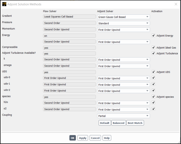
You can specify the methods used for computing the adjoint solutions in the Adjoint Solution Methods dialog box. To open the Adjoint Solution Methods dialog box, click in the Design ribbon tab (Gradient-Based group box).
Design →
Gradient-Based →
Methods...
The Adjoint Solution Methods dialog box shows a side-by-side comparison of the schemes used for the flow solver and for the adjoint solver. Using the same scheme for the adjoint solution and the flow solution yields the most accurate discrete derivative calculation when the adjoint solution is converged. However, not all schemes used for the flow solver are supported for the adjoint solver. In these cases an alternate adjoint scheme must be used. This does not typically lead to severe deterioration of the adjoint results quality. Even if the same scheme is available for the adjoint solver this is not always practical because stability may be reduced with some schemes. Therefore, you can use the drop-down lists under Adjoint Solver to select alternate schemes as needed.
In some cases it may not be desirable to solve the energy adjoint even if energy is solved in the flow solver. For example, consider an incompressible flow where the specified observable does not involve thermal quantities. In this case the adjoint for the energy equation is identically zero, but its inclusion would add an unnecessary numerical burden. You can disable the Adjoint Energy option to avoid solving the energy adjoint.
If the primary flow is a compressible ideal gas, you can specify that the physics of the compressible flow are modeled in the adjoint solver by enabling the Adjoint Ideal Gas option. Enabling this option automatically enables the Adjoint Energy option as well. If the flow is not a compressible ideal gas, it will be treated as being incompressible for the purposes of the adjoint calculation.
When the flow solver uses the generalized -
(GEKO) turbulence model (for details, see
Setting up the Generalized k-ω (GEKO) Model), you can
enable the Adjoint Turbulence option in
order to take the effect of changes to the state of the
turbulence into account when computing sensitivities for the
adjoint calculations, rather than using a frozen turbulence
assumption. This has the following advantages:
The shape sensitivity will be more accurate. This is helpful when high accurate shape sensitivity is needed, such as:
when the design is close to optimal design
when the turbulence state can change significantly with respect to the design changes
when performing optimization with multiple objectives
Sensitivities for GEKO parameters and the curvature correction parameter (CCURV) can be can be calculated at each cell, which can help you to tune the GEKO model.
Including turbulence in the adjoint calculations can make it harder to reach convergence, and will increase the computational and memory cost. For this reason, it is suggested that you only enable turbulence adjoint equations when it is necessary; in most cases, the frozen turbulence assumption should be fine.
Note: You must make sure that the Intermittency Transition Model option was disabled for the flow solution, as it is not supported with adjoint turbulence. However, the Algebraic Transition Model is supported with adjoint turbulence.
When one or multiple user-defined scalar (UDS) transport equations are defined, you can specify the adjoint solver to compute the adjoint for the UDS equations by enabling the Adjoint UDS option. Additionally, when species transport is defined, the adjoint for species transport equations can be computed by enabling the Adjoint species option. After enabling Adjoint UDS or Adjoint species, you can enable the desired UDS or species transport equations to be computed by the adjoint solver. Up to 50 adjoint UDS/adjoint species equations can be enabled.
If the UDS or species transport equations are not necessary for optimization, it is recommended to disable Adjoint UDS and Adjoint species to save time and memory and improve convergence. For example, disabling Adjoint UDS and Adjoint species is recommended for the following scenarios:
When a specific observable is not significantly influenced by UDS or species transport equations.
When the state of UDS or species transport equations do not change significantly with respect to the design changes.
During the early stages of optimization, where achieving sensitivity accuracy is less important.
The adjoint solver utilizes the algebraic multigrid (AMG)
algorithm to solve the correction equations (adjoint
equations) and each AMG block consists of an
N x
N matrix, where
N is the number of adjoint
equations (for more information on the algebraic multigrid
in Ansys Fluent see Algebraic Multigrid (AMG) in the
Fluent theory guide). The adjoint solver can be specified
to be fully coupled or partially coupled by selecting
Full or
Partial respectively in the
Coupled drop-down list. When
Full is selected, all adjoint
equations are coupled within a single AMG block. The adjoint
solver is set to partially coupled by default, and with
Partial selected the adjoint
continuity equation and adjoint momentum equations are
coupled within one AMG block while all other adjoint
equations are solved individually in segregated AMG blocks.
For example, the adjoint solver must solve the following
seven adjoint equations for a 3D turbulence case:
adjoint x-momentum
adjoint y-momentum
adjoint z-momentum
adjoint continuity
adjoint flow rate
adjoint k
adjoint omega
When the adjoint solver is fully coupled,
all of the adjoint equations will be solved within a single
7 x 7 = 49 AMG block. For
the partially coupled adjoint solver, the AMG block for the
adjoint continuity and adjoint momentum equations will be
4 x 4 = 16, while all other
adjoint equations are solved seperately in individual
1 x 1 = 1 AMG blocks.
The significant reduction in the size of the AMG blocks for the partially coupled solver both reduces memory requirements and improves speed per iteration significantly as well, especially when Adjoint Turbulence and/or Adjoint Energy are enabled. Note that while the partially coupled adjoint solver significantly improves performance, the outer convergence may be slightly reduced.
Clicking the button will disable the Adjoint Turbulence equation and set the spatial discretization methods as follows:
Green-Gauss Cell Based for Gradient.
Standard for Pressure .
First Order Upwind for Momentum and Energy (chosen due to their stability).
Partial for Coupling .
Clicking the button will attempt to match the adjoint schemes to the schemes used for the flow solver which should in general provide more accurate calculations at convergence. Where the schemes cannot be matched, the settings will be used.
Clicking the button will provide a balance between stability and accuracy settings. Due to momentum discretization and adjoint turbulence having the largest affect on convergence, the Balanced setting will disable Adjoint Turbulence, set Momentum to First Order Upwind, and use Best Match settings for all other methods.
By default the Rhie-Chow: momentum based flux type is used for the adjoint solver. However, the adjoint solver can be specified to use the same flux type as that of the flow solver using the following text command:
adjoint/expert/match-fluent-flux-type?
By default, the adjoint solver will incorporate 1st order poor mesh numerics used by the conventional flow solver as outlined in Robustness with Meshes of Poor Quality. Poor mesh numerics can be disabled using the following command:
/adjoint/expert/undo-2024r1-default-changes?
The advancement of the adjoint solution to reach a converged solution is an essential part of the analysis. The solution algorithm for the adjoint solver is similar to the coupled pressure-based solver that is available for conventional flow computations in Ansys Fluent.
By default, the adjoint solver advancement settings will be automatically adjusted during calculation to encourage convergence, with initial values determined by the state of the flow solution. If needed, you can adjust the advancement controls in the Adjoint Solution Controls dialog box.
To open the Adjoint Solution Controls dialog box, click in the Design ribbon tab (Gradient-Based group box).
Design →
Gradient-Based →
Solver Controls...
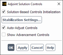
Controls
- Solution-Based Controls Initialization
When enabled, the advancement controls are selected automatically when the adjoint solution is initialized based on the state of the flow.
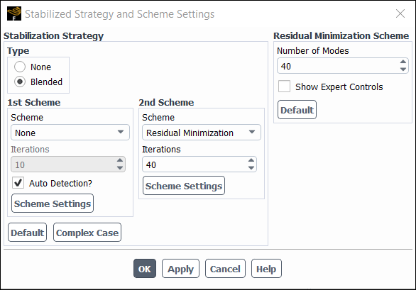
This button opens the Stabilized Strategy and Scheme Settings dialog box, which you can use to define the stabilization strategy, scheme(s), and settings for the adjoint solution. For details, see Stabilization Strategies, Schemes, and Settings.
- Auto-Adjust Controls
When enabled, the convergence of the AMG solver and the adjoint residuals are monitored during solution advancement. Based on the trends observed, the Courant number is automatically adjusted to encourage reliable solution advancement and convergence. This is especially useful when a new type of problem is being solved for which appropriate settings are not initially clear. You can enable or disable Auto-Adjust Controls at any time during the solution.
The Courant number starts at the value you defined in the Advancement Controls group box or the value determined by the Solution-Based Controls Initialization option. When the residual minimization scheme is used, over the first two iterations the Courant number will be increased as high as possible (while still allowing the AMG solver to converge), and will then remain unchanged; for all other setups, the Courant number will be adjusted to ensure the AMG solver converges, with the goal of reducing the AMG residuals at the rate of 1 order of magnitude over 6-8 iterations. Messages will appear as the calculation progresses indicating the adjustments that are being made.
- Show Advancement Controls
This option toggles the visibility of the various advancement controls for direct user specification.
- Advancement Controls
contains the advancement controls.
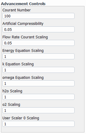
- Apply Preconditioning
Enables solution preconditioning. This is needed for most cases involving turbulent flow. If preconditioning is enabled, additional controls are available.
- Courant Number
A higher number corresponds to a more aggressive advancement of the computation at the risk of instability. Disabling preconditioning corresponds to an infinite Courant number.
- Artificial Compressibility
A nonzero value introduces artificial compressibility into the computation of the adjoint continuity equation. A value of
1.0or less is reasonable.-
Flow Rate Courant Scaling ,
Energy Equation Scaling ,
k Equation Scaling ,
omega Equation Scaling,
species-nScaling, User Scalar n Scaling These values should be larger than zero (default value is
0.05for flow rate and1for all other equations). A smaller value implies a less aggressive algorithm that encourages stability of the AMG linear solver.
- Under-Relaxation Factors
contains the under-relaxation factors.
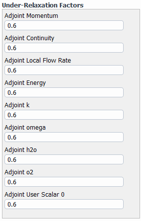
-
Adjoint Momentum,
Adjoint Continuity,
Adjoint Local Flow Rate,
Adjoint Energy ,
Adjoint k, Adjoint
omega, Adjoint
species-n, Adjoint User Scalar n Each of these can be set to a value between
0.0to1.0. A higher value leads to a more aggressive algorithm that is less likely to be stable. A value of1.0for each can be used for some simple cases without difficulty.
-
Adjoint Momentum,
Adjoint Continuity,
Adjoint Local Flow Rate,
Adjoint Energy ,
Adjoint k, Adjoint
omega, Adjoint
- Algebraic Multigrid
contains the algebraic multigrid controls.
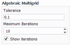
- Tolerance
The tolerance used for judging convergence.
- Maximum Iterations
The maximum number of inner iterations of the AMG solver.
- Show Iterations
If enabled, a more verbose iteration history is printed in the text console during iterations. The details of the inner iteration can be useful when deciding on appropriate Courant Number, Artificial Compressibility, and Flow Rate Courant Scaling. If many inner iterations are needed, or if the inner iterations diverge, this signals that a reduction in Courant Number may be needed. Alternatively, an increase in Artificial Compressibility or a reduction in the Flow Rate Courant Scaling may be sufficient for the AMG iterations to converge.
For an overview of when stabilization is needed and descriptions of the available schemes, see Adjoint Solver Stabilization. You can define a stabilization strategy in the Stabilized Strategy and Scheme Settings dialog box, which is opened by clicking the button in the Adjoint Solution Controls dialog box.
Selecting None from the Type list in the Stabilization Strategy group box on the left allows you to select a single stabilization method to be used throughout the calculation, or none at all. You specify your preference using the Scheme drop-down list in the Current Scheme group box, then click the button to define the scheme settings on the right.
Alternatively, you can select Blended from the Type list in the Stabilization Strategy group box on the left, so that either no scheme (None) or the Dissipation scheme is applied at the beginning of the calculation, depending on your selection from the Scheme drop-down list in the 1st Scheme group box; then a second scheme (the Residual Minimization scheme) is used for the remainder of the calculation. If you enable the Auto Detection? option, the first scheme will be used until divergence or slow convergence in the adjoint residual is detected; otherwise, you specify an explicit number of Iterations to be run before switching to the second scheme. The latter can be useful for cases that take a long time to diverge or show signs of slow convergence with the first scheme, as you can force an early switch to the residual minimization scheme (which generally converges quickly). You can also specify the maximum number of Iterations to allow for the 2nd Scheme, as the residual minimization scheme can be expensive on a per iteration basis. Note that settings used for the dissipation and residual minimization schemes are defined within the Dissipation Scheme and Residual Minimization Scheme group boxes on the right, which will appear after clicking the button in the 1st Scheme and 2nd Scheme group boxes, respectively. The controls for each scheme are described in the sections that follow.
Note: After your first calculation is complete, the second stabilization scheme will be used at the start of all subsequent calculations, unless you click the button in the Run Adjoint Calculation dialog box prior to calculating. Initializing the strategy is recommended when there is an operation that will cause a residual jump (such as morphing the mesh), as the first scheme can resolve some of the modes more efficiently.
When using the Blended strategy,
note that you can use the
button to revert
any changes you have made to the settings. You can
also use the
button to use settings that are more appropriate for
complex cases that would benefit from the initial
use of the dissipation scheme to damp local
diverging modes, before switching to the residual
minimization scheme; note that for some cases, you
may need to increase the
Iterations for the
dissipation scheme or increase the damping factor in
the Dissipation Scheme group
box (for example, to 100)
to allow the scheme to fully damp the modes.
The stabilization settings for each scheme are described in the following sections:
The dissipation scheme operates by introducing nonlinear damping strategically into the calculation domain. The strategy is intended to provide minimal intervention in order to damp the growth of instabilities that lead to adjoint solution divergence. A marker is tracked, based on the state of the adjoint solution, and the damping is applied directly to the adjoint solution in regions where the marker becomes large.
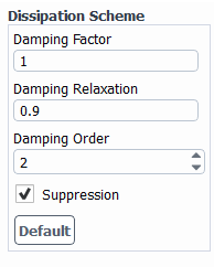
When Dissipation is selected from the Scheme drop-down list within the Current Scheme or 1st Scheme group box (depending on the specified Stabilization Strategy), you can then click the button to open the Dissipation Scheme group box on the right and define the following settings:
- Damping Factor
The overall level of dissipation is proportional to this value although the damping level is determined ultimately through a nonlinear process.
- Damping Relaxation
The damping relaxation can be used to control the rate at which the dissipation is updated as the adjoint solution progresses. As you decrease the value from 1, the rate at which the dissipation is updated is decreased.
- Damping Order
The spatial order of the dissipation. A higher order leads to more intense and localized damping. This can typically be set to be one order larger than the adjoint calculation spatial order.
- Suppression
As part of the dissipation scheme, the growth of instabilities is stopped by the effect of the dissipation; enabling the Suppression option ensures that these undesirable patterns will then also decay as the calculation progresses.
Since the order of discretization of the dissipation scheme is usually set higher than the adjoint, the formal order of accuracy of the adjoint solution is unaffected by the addition of dissipation. However, regions of intense dissipation can appear for some cases when using this scheme. This can sometimes appear as isolated spots and streaks in the adjoint solution on surfaces. The scale of these features is such that they are often easily smoothed during postprocessing to generated design changes.
The residual minimization scheme operates by building a Krylov subspace and using it to build a solution with minimum residual.
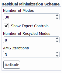
When Residual Minimization is selected from the Scheme drop-down list within the Current Scheme or 2nd Scheme group box (depending on the specified Stabilization Strategy), you can then click the button to open the Residual Minimization Scheme group box on the right and define the following settings:
- Number of Modes
This specifies the number of modes in the Krylov subspace used to approximate the solution. Increasing the number of modes will increase the convergence and reduce the final residual. The convergence rate may increase sharply when the number of modes is larger than a certain threshold. Note that the memory needed for this scheme is proportional to (number of adjoint equations) * (number of modes + number of recycled modes). You should ensure that you have enough memory for the value you enter here; an estimation of the additional memory needed at the peak is printed in the console when you click .
- Show Expert Controls
Enabling this option reveals the expert controls described below, so that you can adjust them from the default values.
- Number of Recycled Modes
This specifies the number of modes that are selected, stored, and used for the next iteration to speed up the convergence. The default value is a quarter of the number of modes.
For the initial step of the residual minimization scheme, the number of sub-iterations is equal to the number of modes; for later steps, it is the difference of the number of modes and the number of recycled modes. Therefore, increasing the number of recycled modes will reduce the number of sub-iterations for each main iteration; while this relation is straightforward, the effect on the overall convergence ratio is not, as it is case dependent.
- AMG Iterations
This specifies the fixed number of AMG iterations in each sub-iteration. Increasing the number may improve the overall convergence, but it also increases the time for each sub-iteration.The residual minimization scheme is unique in that it does not require the AMG solver to reduce the inner residual by at least one order; it only requires that the AMG solver not be diverging. In fact, a more aggressive setting of preconditioning may slow down the inner AMG convergence, but improve the overall outer loop convergence. Such an improvement can be significant.
Note: The following tips can be helpful when using the residual minimization scheme:
It is highly recommended that you first run the adjoint solver without a stabilization scheme until the adjoint residual starts to diverge, and then enable the residual minimization scheme. The first run damps out many stable modes in the adjoint residual and reduces the number of modes required in the residual minimization scheme. Note that this can easily be done by selecting the Blended strategy in the Stabilization Strategy group box.
The overall adjoint residual will be printed in the console. The residual should either decrease monotonically or stall within each main iteration or between main iterations. If you do not see such behavior, click the button in the Run Adjoint Calculation dialog box to initialize the scheme.
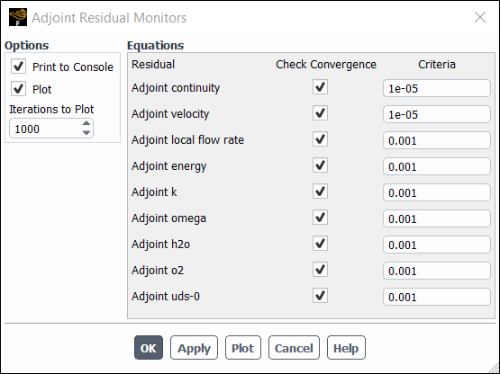
The progress of the iterations of the adjoint solver and the monitoring of the convergence is controlled in the Adjoint Residual Monitors dialog box. This dialog box is accessed by clicking in the Design ribbon tab (Gradient-Based group box).
Design →
Gradient-Based →
Monitors...
The steps to define the monitor behavior are as follows:
Decide whether or not the residuals are to be printed in the console by setting the Print to Console check box as desired.
Decide whether or not the residuals are to be plotted in the main window by setting the Plot check box as desired.
Set how many iterations are to be shown in the residual curves that are plotted in the Iterations to Plot field.
Enable and/or disable those values that are to be used as criteria for convergence, and set the Criteria in each case. The options are to test the residuals for the following equations: Adjoint continuity, Adjoint velocity, Adjoint local flow rate , Adjoint energy, Adjoint k, Adjoint omega, Adjoint
species-n, and/or Adjoint uds-n.
Click the or buttons to confirm that the settings are acceptable. Clicking will cause existing adjoint residuals to be plotted in the main graphics window.
If the adjoint calculation does not converge properly, you can print and/or postprocess the adjoint equation residuals, as this can provide useful information for the diagnosis of convergence issues. Convergence issues can be caused by:
Flow instability such as high shear flow, flow separation, or reverse flow
Poor mesh quality
A specific boundary condition
Unsupported models in Fluent, as mentioned in the warning message
To help understand the cause of your particular convergence issue, you can enable the following text commands prior to running the adjoint calculation:
adjoint→expert→diagnosis→print-residuals-by-zoneThis text command specifies that the residuals are printed in the console during the calculation in a format that allows you to see if the high residual is located at a specific boundary zone.
adjoint→expert→diagnosis→retain-cell-residualsThis text command saves the residuals as field variables that can be postprocessed, so that you can visualize the high residual region to check if any of the previously mentioned reasons are the cause of convergence issues. Occasionally, the divergence only occurs locally, and most of the residual is located at a small region. In this case, even though the adjoint residual value is not low, the adjoint solution can still be used to improve your design if you can avoid morphing that region.
adjoint→expert→diagnosis→print-residuals-by-distributionThis text command specifies that the distribution of the residuals is printed in the console during the calculation, so that you can see if a high percentage of the residuals is located in a small number or percentage of cells.
Note: After setting up the text user command, you need to run at least 1 adjoint iteration to print / save the residual or receive a message.
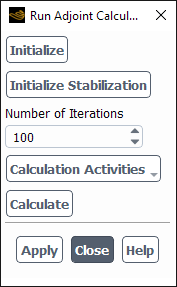
Initialization and execution of the adjoint solver is accomplished in the Run Adjoint Calculation dialog box. This dialog box is accessed by clicking in the Design ribbon tab (Gradient-Based group box).
Design →
Gradient-Based →
Calculate...
The function of this dialog box is as follows:
sets the value of the adjoint velocity and pressure to zero everywhere in the problem domain.
initializes the stabilization strategy, such that the first stabilization scheme is used at the start of the next calculation rather than continuing to use the second stabilization scheme. This button is only available when the blended stabilization strategy is used. For details, see Stabilization Strategies, Schemes, and Settings.
clears all of the unstable modes that have been identified in calculations using the stabilization scheme, but leaves the adjoint solution unchanged. This button is only available when the residual minimization scheme is enabled.
sets the number of iterations for the calculation. Note that if you are using a blended stabilization strategy, the calculation may end sooner if the total of the iterations you specified in the Stabilized Strategy and Scheme Settings dialog box (described in Stabilization Strategies, Schemes, and Settings) is less than the value you enter here.
allows you to access dialog boxes so you can set up various tasks that can be performed during the adjoint calculation. This drop-down list provides the following selections:
- Autosave...
opens the Adjoint Autosave dialog box. For details, see Automatic Saving of Case and Data Files During an Adjoint Calculation.
- Execute Commands...
opens the Execute Commands Dialog Box , which you can use to set up commands to be executed during the adjoint calculation (such as postprocessing commands that export fields). For details, see Executing Commands During the Calculation. Note that once you have opened this dialog box from Run Adjoint Calculation dialog box, the following selections become available in the When drop-down list:
- Adjoint Iteration
This specifies that execution of the command is based on the adjoint iteration. It is executed immediately before each adjoint advancement step.
- Design Iteration
This specifies that execution of the command is based on the design iteration. It is executed after the design calculation and before any animation recording, both of which are before the morphing of the mesh.
Note that unexpected behavior may result if the executed command changes settings for the adjoint calculation.
advances the adjoint solver by the Number of Iterations specified in the adjacent field.
Depending on the monitor settings, the residuals may be printed in the console and/or plotted in the main graphics window.
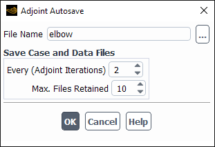
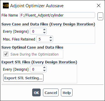
The Adjoint Autosave dialog box allows you to specify automatic saving of case and data files at specified intervals during an adjoint calculation. This dialog box is accessed by selecting from the Calculation Activities drop-down list in the Run Adjoint Calculation dialog box (described in Running the Adjoint Calculation).
The function of this dialog box is as follows:
- File Name
specifies the root name for the files that are saved. The adjoint iteration and an appropriate suffix will be added to the specified root name; by default, the suffix will be
.cas.h5or.dat.h5.- Save Case and Data Files
provides the following controls:
- Every (Adjoint Iterations)
specifies the frequency (in adjoint iterations) with which case and data files are saved. The default value is set to
0, indicating that no automatic saving is performed.- Max. Files Retained
specifies the maximum number of case and data files that can be retained. If you have constraints on the disk space, you can restrict the number of files to be saved using this field. After saving the specified number of files, Ansys Fluent will overwrite the earliest existing files. The default value for this field is
5. Entering a value of0ensures that all of the files are retained.
Adjoint solution data can be postprocessed so that it provides both qualitative and quantitative views of the effect of many types of change that may be imposed on a system. While shape changes are often of particular interest there is a very rich data set, one as large as the original flow field, available for exploration. Postprocessing tools are provided with the intention of permitting the adjoint data to be mined in such a way that it provides useful supporting information for an engineer who is making design decisions for a system, or has questions about the reliability of the original flow calculation.
Since the Ansys Fluent adjoint solver is a discrete adjoint solver, the primitive adjoint solution data provides sensitivity to changes cell-wise for the computational mesh. Normalization of these results by the cell volume provides a mesh-independent view into the data set.
Information regarding postprocessing the adjoint solutions can be found in the following sections:
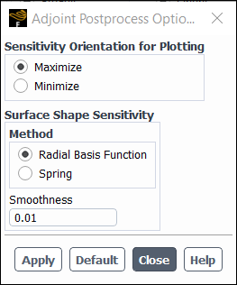
Settings for postprocessing adjoint sensitivity data is accomplished in the Adjoint Postprocess Options dialog box. This dialog box is accessed by clicking in the Design ribbon tab (Gradient-Based group box).
Design →
Gradient-Based → Postprocess
Options...
The function of this dialog box is as follows:
- Sensitivity Orientation for Plotting
provides the following controls:
- Maximize
specifies changes in the direction of positive sensitivities to increase the value of the observable.
- Minimize
specifies changes in the direction of negative sensitivities to decrease the value of the observable.
When defining Sensitivity Orientation for Plotting, a standard rule of thumb can be applied: if you want to improve the solution using the Maximize or Minimize settings, then follow the direction of the sensitivity vectors. Another standard rule of thumb can also be applied for postprocessed scalars: if you want to improve the solution, then increase values where the sensitivity is positive and/or decrease values where the sensitivity is negative.
- Method
By default the Radial Basis Function is used to calculate and smooth the surface shape sensitivity. However, you can enable the Spring option to reduce memory and computational cost. The spring method assumes that the interior mesh motion is governed by the surface mesh motion, using the spring analogy equation. The adjoint of the spring equation is then solved to back propagate the interior shape sensitivity onto the surface, resulting in a physical shape sensitivty that is not smoothed. To smooth the shape sensitivty, Laplace surface smoothing is used based on the defined smoothness settings to achieve a smoothed surface shape sensitivity.
- Smoothness
Specifies the smoothness of the Sensitivity to Surface Shape field, which is smoothed using either the radial basis function (when Radial Basis Function is enabled), or by solving an adjoint spring equation (when Spring is enabled). Decreasing this value will accentuate the effect of local geometric features on the Sensitivity to Surface Shape field.
Adjoint solution data can be postprocessed using standard Ansys Fluent postprocessing tools including contours, vectors, xy-plots, histograms, and surface and volume integrals.
Under Sensitivities... (for example, in the Contours dialog box), you can find the following fields:
- Magnitude of Sensitivity to Body Forces (Cell Values)
This field is the magnitude of the adjoint velocity primitive field. This field can be interpreted as the magnitude of the sensitivity of the observable to body force per unit volume. It can be used to identify regions in the domain where small changes to the momentum balance in the flow can have a large or small effect on the observable. This field is often observed to be large, for example, upstream of a body for which drag sensitivity is of interest, with the field diminishing in the upstream direction. This indicates the interference effect for an object positioned at various locations upstream of the object of interest.
- Sensitivity to Body Force X-Component (Cell Values), Sensitivity to Body Force Y-Component (Cell Values), and Sensitivity to Body Force Z-Component (Cell Values)
These are the components of the adjoint velocity primitive field. These fields can be interpreted as the magnitude of the sensitivity of the observable to components of a body force per unit volume. Consider a body force distribution, expressed as a force per unit volume. The volume integral of the vector product of that distribution with the components of this field gives a first-order estimate of the net effect of the body force on the observation.
- Sensitivity to Mass Sources (Cell Values)
This field is the primitive adjoint pressure field. This field can be interpreted as the sensitivity of the observable with respect to mass sources or sinks in the domain. Consider a mass source / sink distribution, expressed as mass flow rate per unit volume. The volume integral of that distribution, weighted by the local value of this field, gives the effect of the sources / sinks on the observation. When plotted on a boundary, this field indicates the effect of the addition or removal of fluid from the domain upon the quantity of interest. It is important to note that in this scenario the effect of the momentum of the fluid that is added or removed is not taken into account. The boundary velocity sensitivity should be plotted if that effect is also of interest.
- Sensitivity to Energy Sources (Cell Values)
This field is available when the energy adjoint equation is solved and is the primitive adjoint temperature field. It can be interpreted as the sensitivity of the observable with respect to the thermal energy sources or sinks per unit volume in the domain.
- Sensitivity to Turbulent Kinetic Energy Sources (Cell Values)
This field is available when the turbulence adjoint equations are solved and is the sensitivity of the observable with respect to the turbulent kinetic energy (
) sources per unit volume in the domain.
- Sensitivity to Specific Dissipation Rate Sources (Cell Values)
This field is available when the turbulence adjoint equations are solved and is the sensitivity of the observable with respect to the specific dissipation rate (
) sources per unit volume in the domain.
- Sensitivity to Scalar-n Sources (Cell Values)
This field is available when the specified UDS adjoint equations are solved and is the sensitivity of the observable with respect to the user-defined scalar sources per unit volume in the domain.
- Sensitivity to
species-nSources (Cell Values) This field is available when the specified species adjoint equations are solved and is the sensitivity of the observable with respect to the species sources per unit volume in the domain.
- Artificial Dissipation
This field is available when the adjoint dissipation stabilization scheme is enabled and shows the location and amount of the nonlinear damping that has been introduced to damp the growth of instabilities that lead to adjoint solution divergence.
- Sensitivity to Viscosity
This field shows the sensitivity of the quantity of interest to variations in the turbulent effective viscosity for a turbulent problem, or the laminar viscosity in a laminar case. The sensitivity is normalized by the cell volume to account for cell size variations in the mesh.
- Shape Sensitivity Magnitude
This field is the magnitude of the sensitivity of the observable with respect to a deformation applied to the mesh (both boundary and interior mesh). When plotted on the surface of a body the locations where this quantity is large indicates where small changes to the surface shape can have a large effect on the observable of interest. If the shape sensitivity magnitude is small then the effect of shape changes in this region can be expected to have a small effect on the observable of interest. When viewing this field, it is often observed that the magnitude varies by many orders of magnitude. Contour plots will clearly draw attention to regions with the highest sensitivity (often sharp edges and corners). However, it should be remembered that a relatively small surface movement that is distributed over a large area can have a cumulative effect that is large.
- Normal Shape Sensitivity
This field shows the normal component of the shape sensitivity. A positive value indicates an orientation directed into the domain, while a negative value indicates that the shape sensitivity is oriented outwards from the domain. This field eliminates the component of the vector shape sensitivity field that lies in the plane of the wall.
- Normal Surface Shape Sensitivity
This field shows the normal component of the surface shape sensitivity, which is an accumulation of surrounding nodal sensitivities to the surface. A positive value indicates an orientation directed into the domain, while a negative value indicates that the surface shape sensitivity is oriented outwards from the domain. The accumulation of surrounding nodal sensitivities produces a more accurate representation of the physical surface sensitivity when compared to the Normal Shape Sensitivity field which uses raw nodal sensitivity data. The normal surface shape sensitivity field is smoothed using the radial basis function and smoothness settings can be adjusted within the Adjoint Postprocess Options dialog box.
- Normal Optimal Displacement
This field shows the normal component of the optimal displacement computed from the adjoint design tool calculation. This field is defined only for portions of walls lying within the control-volume specified for morphing. A positive value of displacement indicates that the surface will be displaced into the flow domain, whereas a negative value of displacement corresponds to wall movement outwards from the flow domain. This field eliminates the component of the optimal displacement vector that lies in the plane of the wall.
- Optimal Displacement X-Component , Optimal Displacement Y-Component , Optimal Displacement Z-Component (in 3D)
These fields are the individual components of the optimal displacement computed from the adjoint design tool calculation. These fields are defined only for portions of walls lying within the control-volume specified for morphing.
- log10(Shape Sensitivity Magnitude)
In view of the large range of values possible for the shape sensitivity magnitude, a convenience function that plots
of the magnitude is provided. This allows the importance of the surfaces in a domain to be ranked more easily based on how they affect the observation of interest when they are reshaped.
- Shape Sensitivity X-Component, Shape Sensitivity Y-Component, and Shape Sensitivity Z-Component (in 3D)
These fields are the individual components of the sensitivity of the observable of interest with respect to the mesh node locations. It is plotted as cell data and is computed as the average of the nodal sensitivities for a given cell, divided by the cell volume. Note that for this discrete adjoint solver the sensitivity of the result with respect to node locations both on and off boundaries is computed. The normalization by cell volume indicates that the fields that are plotted are the weighting factors for a continuous spatial deformation field. (Note that the nodal sensitivity data itself is used when mesh morphing is performed, and predictions about the effect of shape changes are made.)
- Sensitivity to Boundary X-Velocity , Sensitivity to Boundary Y-Velocity, and Sensitivity to Boundary Z-Velocity (in 3D)
These fields are defined on those boundaries where a user-specification of a boundary velocity is made for the original flow calculation. This includes no-slip walls. The field shows how sensitive the observable of interest is to changes in the boundary velocity at any point. It is interesting to note that even though the original boundary condition specification may be for a uniform velocity on the domain boundary, the effect of a non-uniform velocity perturbation is available. The effect of any specific boundary velocity change can be estimated as an integral of the vector product of the change to the velocity with the plotted sensitivity field. A plot of this quantity on a velocity inlet, for example, can be very useful for assessing whether or not the inlet is positioned too close to key parts of the system. That is, it addresses the question of whether or not the flow domain is too small to achieve a successful computation of the performance measure of interest. Viewing this field will also indicate whether or not the assumption of a uniform inflow is adequate.
- Sensitivity to Boundary Pressure
This field is defined on boundaries where there is a user-specified pressure as part of a boundary condition, such as on a pressure outlet. The field shows the sensitivity of the observation of interest to variations in the boundary pressure across the flow boundary. It is interesting to note that even though the original boundary condition specification may be for a uniform pressure on the domain boundary, the effect of a non-uniform pressure perturbation is available, The effect of any specific boundary pressure change can be estimated as an integral of the product of the change to the pressure with the plotted sensitivity field. Viewing this field will also indicate whether or not the assumption of a uniform pressure is adequate for the simulation.
- Sensitivity to Boundary Temperature
This field is available when the energy adjoint equation is solved and is defined on boundaries where a temperature boundary condition is applied. This includes walls, velocity inlets, mass-flow inlets, pressure inlets, pressure far-field boundaries, and pressure outlets where a backflow temperature may be specified. The field shows the sensitivity of the observation of interest to variations in the boundary temperature across the boundaries. Note that even if the original boundary condition specification is for a uniform temperature on the boundary, the effect of a non-uniform temperature perturbation is available. The effect of any specific boundary temperature change can be estimated as an integral of the product of the change to the temperature with the plotted sensitivity field. This field can be used to indicate whether or not the assumption of a uniform temperature is adequate for the simulation.
- Sensitivity to Boundary Heat Flux
This field is available when the adjoint energy equation is solved and is defined on walls where a heat flux boundary condition is imposed. The field shows the sensitivity of the observation of interest to variations in the boundary heat flux through the wall. Its properties are analogous to those of Sensitivity to Boundary Temperature.
- Sensitivity to Scalar-n Boundary Value
This field is available when the specified UDS adjoint equations are solved and is defined on boundaries where a user-defined scalar boundary condition with specified value is imposed. The field shows the sensitivity of the observation of interest to variations in the user-defined scalar boundary value across the flow boundary.
- Sensitivity to Scalar-n Boundary Flux
This field is available when the specified UDS adjoint equations are solved and is defined on boundaries where a user-defined scalar boundary condition with specified flux is imposed. The field shows the sensitivity of the observation of interest to variations in the user-defined scalar boundary flux across the flow boundary.
- Sensitivity to
species-nBoundary Value This field is available when the species adjoint equations are solved and is defined on boundaries where a species boundary condition with a specified mass fraction is imposed. The field shows the sensitivity of the observation of interest to variations in the species mass fraction across the flow boundary.
- Sensitivity to
species-nBoundary Flux This field is available when the species adjoint equations are solved and is defined on boundaries where a species boundary condition with specified flux (mass) is imposed. The field shows the sensitivity of the observation of interest to variations in the species boundary flux (mass) across the flow boundary.
- Sensitivity to Flow Blockage
This field is provided as a convenient tool for identifying portions of the flow domain where the introduction of blockages or obstructions in the flow can affect the observation of interest. Consider a blockage in the flow that generates a reaction force on the flow that is proportional to the local flow speed, and acting in the opposite direction to the local flow:
where
is a local coefficient for the reaction force. The local contribution of this force on the observation of interest is determined by the vector product of this force with the adjoint velocity field. The flow blockage field that is plotted is
, namely the negative of the vector product of the flow velocity and the adjoint velocity (Cell Value).
- Sensitivity to GEKO CSEP
This field is available when the turbulence adjoint equations are solved and is the sensitivity of the observable with respect to the
parameter, which is used to optimize flow separation from smooth surfaces.
- Sensitivity to GEKO CNW
This field is available when the turbulence adjoint equations are solved and is the sensitivity of the observable with respect to the
parameter, which is used to optimize flow in non-equilibrium near wall regions (such as heat transfer or
).
- Sensitivity to GEKO CMIX
This field is available when the turbulence adjoint equations are solved and is the sensitivity of the observable with respect to the
parameter, which is used to optimize strength of mixing in free shear flows.
- Sensitivity to GEKO Blending Function
This field is available when the turbulence adjoint equations are solved and is the sensitivity of the observable with respect to the blending function,
, which is used to deactivate GEKO parameters inside boundary layers.
- Sensitivity to CCURV
This field is available when the turbulence adjoint equations are solved for a case in which the Curvature Correction option is enabled in the Viscous Model dialog box. It is the sensitivity of the observable with respect to the curvature correction parameter, CCURV , which is used to optimize the strength of the curvature correction if needed for a specific flow.
- Adjoint GEKO CSEP
This field is available after performing gradient-based turbulence model optimization within the Gradient-Based Optimizer and is the optimized
parameter, which is used to optimize flow separation from smooth surfaces.
- Adjoint GEKO CNW
This field is available after performing gradient-based turbulence model optimization within the Gradient-Based Optimizer and is the optimized
parameter, which is used to optimize flow in non-equilibrium near wall regions (such as heat transfer or
).
- Adjoint GEKO CMIX
This field is available after performing gradient-based turbulence model optimization within the Gradient-Based Optimizer and is the optimized
parameter, which is used to optimize strength of mixing in free shear flows.
- Adjoint GEKO BF
This field is available after performing gradient-based turbulence model optimization within the Gradient-Based Optimizer and is the optimized blending function (
), which is used to deactivate GEKO parameters inside boundary layers..
- Adjoint GEKO CSEP (Trained)
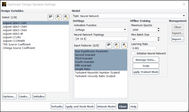
This field is available after performing Offline training of the neural network turbulence model within the Optimizer Design Variables dialog box, and is the trained
parameter.
- Adjoint GEKO CNW (Trained)
This field is available after performing Offline training of the neural network turbulence model within the Optimizer Design Variables dialog box, and is the trained
parameter.
- Adjoint GEKO CMIX (Trained)
This field is available after performing Offline training of the neural network turbulence model within the Optimizer Design Variables dialog box, and is the trained
parameter.
- Adjoint GEKO BF (Trained)
This field is available after performing Offline training of the neural network turbulence model within the Optimizer Design Variables dialog box, and is the trained blending function parameter (
).
- Non-Equilibrium Parameter
This field is available when the Neural Network Model has been applied for turbulence model optimization within the Optimizer Design Variables dialog box, and is the Non-Equilibrium Parameter flow feature.
- Second Invariant
This field is available when the Neural Network Model has been applied for turbulence model optimization within the Optimizer Design Variables dialog box, and is the Second Invariant flow feature.
- Third Invariant
This field is available when the Neural Network Model has been applied for turbulence model optimization within the Optimizer Design Variables dialog box, and is the Third Invariant flow feature.
- Fourth Invariant
This field is available when the Neural Network Model has been applied for turbulence model optimization within the Optimizer Design Variables dialog box, and is the Fourth Invariant flow feature.
- Fifth Invariant
This field is available when the Neural Network Model has been applied for turbulence model optimization within the Optimizer Design Variables dialog box, and is the Fifth Invariant flow feature.
- Length Ratio
This field is available when the Neural Network Model has been applied for turbulence model optimization within the Optimizer Design Variables dialog box, and is the length ratio flow feature.
- Turbulent Reynolds Number (Scaled)
This field is available when the Neural Network Model has been applied for turbulence model optimization within the Optimizer Design Variables dialog box, and is the scaled turbulent reynolds number flow feature.
- Turbulent Viscosity Ratio (Scaled)
This field is available when the Neural Network Model has been applied for turbulence model optimization within the Optimizer Design Variables dialog box, and is the scaled turbulent viscosity ratio flow feature.
- Mahalanobis distance
This field is available when the Neural Network Model is selected for turbulence model optimization within the Optimizer Design Variables dialog box. Large values for the Mahalanobis distance suggest large deviations in flow features compared to the training data results.
- Adjoint Local Solution Marker
This field intended for expert users, can be plotted to identify those portions of the flow domain where the stabilized adjoint solution advancement scheme is applied. It is preferable to plot this with the Node Values disabled in the Contours dialog box. In this case, the Adjoint Local Solution Marker will take a value between 0 and 1. The
Mode Amplitude
                                        Cutoff
defined through theadjoint/controls/stabilizationtext command defines the lower bound for cells where the stabilized scheme is applied.- Adjoint X-Velocity Residual
This field is available for users using the adjoint diagnosis and is the x-component of the residual of the adjoint momentum equation in each cell.
- Adjoint Y-Velocity Residual
This field is available for users using the adjoint diagnosis and is the y-component of the residual of the adjoint momentum equation in each cell.
- Adjoint Z-Velocity Residual
This field is available for users using the adjoint diagnosis and is the z-component of the residual of the adjoint momentum equation in each cell.
- Adjoint Continuity Residual
This field is available for users using the adjoint diagnosis and is the residual of the adjoint continuity equation in each cell.
- Adjoint Local Flow Rate Residual
This field is available for users using the adjoint diagnosis and is the residual of the adjoint local flow rate equation in each cell.
- Adjoint Energy Residual
This field is available for users using the adjoint diagnosis and is the residual of the adjoint energy equation in each cell.
- Adjoint Turbulent Kinetic Energy Residual
This field is available for users using the adjoint diagnosis and is the residual of the adjoint turbulent kinetic energy equation in each cell.
- Adjoint Specific Dissipation Rate Residual
This field is available for users using the adjoint diagnosis and is the residual of the adjoint specific dissipation rate in each cell.
The surface shape-sensitivity fields contain the derivatives of the chosen observable with respect to the position of the walls of the problem.
In the Vectors dialog box, under Vectors of, you can find the following custom vector fields:
- Sensitivity to Body Forces (Cell Values)
This vector field shows how sensitive the observable of interest is to the presence of body forces within the flow. A body force that locally has a component in the direction of the body-force sensitivity vector will lead to an increase in the observation of interest. The larger the sensitivity vector, the larger the effect that a body force can have on the observation of interest. The first-order effect of a body force distribution per unit volume can be computed as a volume integral of the vector product of the body force distribution with this field.
- Sensitivity to Shape
This vector field shows the postprocessed adjoint solution, independent of any morphing settings, that defines the sensitivity of the observable of interest to movement of the walls. Deformation of a wall where this vector is large can be expected to have a significant effect on the observable. In contrast, deformations of the wall in locations where this vector is small in magnitude, to first order, will have no effect on the observable.
- Sensitivity to Surface Shape
This vector field shows the postprocessed adjoint solution, independent of any morphing settings, and accumulates the sensitivites of surrounding nodes to the surface. The accumulation of surrounding nodal sensitivities produces a more accurate representation of the physical surface sensitivity when compared to the Sesnitivity to Shape vector field which uses raw nodal sensitivity data. Surface shape sensitivity is smoothed using the radial basis function and smoothness can be adjusted within the Adjoint Postprocess Options dialog box.
- Optimal Displacement
The optimal displacement field is defined once a design change has been computed using the Design Tool. This vector field shows the optimal displacement based on the design goals that have been specified and any prescribed boundary motions. Note that when plotting this vector field, if the Auto Scale option is deselected, and the vector Scale option is set to 1, then the vectors as shown display the absolute displacement that will occur.
- Sensitivity to Boundary Velocity
This sensitivity field is defined on boundaries where velocities are specified as an input for the boundary condition. This includes no-slip, and slip walls. When plotted, this field illustrates where a change to the boundary velocity can affect the observation of interest. When plotted on a wall, it shows how the imposition of a nonzero velocity condition on the wall will affect the observation. This can include movement in the plane of the wall itself. When plotted, for example on a velocity inlet, this field illustrates how local adjustments to the velocity of the incoming flow affect the observation of interest. Integrating a potential change to the velocity field, weighted by this sensitivity field over the boundary provides a first order estimate of the effect of the change on the observation of interest.
- Sensitivity to Boundary Mass Flux
This sensitivity field that can be used to visualize the effect of adding or removing fluid via a wall-normal jet. This can be used, for example, to identify regions on walls where the introduction of suction could have a significant effect on the observable that has been specified. A plot of the Sensitivity to Boundary Velocity in general provides a richer view, but sometimes at the expense of the clarity of the visualization.
The computed adjoint solution can provide sensitivity information for individual boundary condition settings through the Adjoint Reporting dialog box. This dialog box is accessed by clicking in the Design ribbon tab (Gradient-Based group box).
Design →
Gradient-Based →
Reporting...
Boundary condition sensitivity data is retrieved as follows:
Select a single boundary of the problem in the Boundary Choice selection box.
Click Report to see the boundary condition settings and the sensitivity of the observable with respect to those settings. An example of a report is shown below:
Velocity inlet id 5
Velocity magnitude = 4.000000000e+01 (m/s),
Sensitivity = 5.429127866e+01 ((n)/(m/s))
In this case, the report shows that for every change of the boundary velocity by 1 m/s, a change in the predicted observable (in this case a force) of 54.2 N is expected. This prediction is based on a linear extrapolation.
Click Write... to write the report for the selected boundary to a file.
Tools to modify the boundary and interior mesh of the problem based on the adjoint solution are provided in the Design Tool dialog box. The Design Tool uses computed adjoint sensitivity data to find an optimal design change satisfying one or more goals or constraints, and to predict the resulting changes in observable values. Among the goals that can be specified in the Design Tool are:
minimization, maximization, or targeted changes of single or multiple observable values
prescribed forms of deformation for selected geometry
general constraints on deformations including restrictions on direction of motion, symmetry, and boundary conditions.
equality and/or inequality constraints on geometry (fixed walls, bounding boxes, and so on).
The general procedure to use the Design Tool is as follows.
Open the Design Tool by clicking in the Design ribbon tab ( Gradient-Based group box).
Design → Gradient-Based → Design Tool...
Select the appropriate Morphing Method and Constraint Method for your problem.
If your problem contains some design constraints such as fixed zones and bounded-by-surface conditions, the Enhanced Constraint Method with the Polynomials Morphing Method or Radial Basis Function is recommended. The Enhanced constraint method can provide a better balance during mesh morphing compared to the Standard constraint method in terms of efficiency and accuracy when handling design conditions. Additionally, the Enhanced constraint method can produce a better quality mesh than the Standard constraint method and setup of the design tool is greatly simplified.
Note: The Enhanced Constraint Method is only available for the Radial Basis Function and Polynomials morphing methods.
Prior to using the Enhanced constraint method, you must ensure that there are no limitations when using this method for your problem as outlined in Smoothing and Mesh Morphing.
When Standard is selected for the Constraint Method:
Radial Basis Function is generally recommended for the Morphing Method if you prefer mesh quality and have some design conditions.
If no design conditions are present, including no zones intended to stay fixed in the morphing region, Polynomials is recommended due to its computational speed and good mesh quality.
Direct Interpolation is recommended if you have many design conditions.
For details on how they calculate the displacement of the mesh nodes and their relative merits, see Smoothing and Mesh Morphing.
Select those boundaries that are free to be deformed in the Modifiable Zones field on the Design Change tab. Boundaries that are not selected in this box that intersect the control volume will be constrained not to move. This is useful if there are walls which, for design reasons, must not move.
Note:If you have a two-sided wall that you want to deform, it is recommended that you select both the wall and the corresponding wall-shadow.
When using the Direct Interpolation morphing method, you must ensure that none of the zones involved in a non-conformal mesh interface are selected.
Define the region that will be modified in the Region tab. (Defining the Region for the Design Change)
Define conditions on the deformation region such as number of control points, symmetry, directional invariance, and boundary continuity. (Defining Region Conditions)
Export the sensitivities from the adjoint solution for each observable of interest. (Defining Observable Objectives)
Import the sensitivity data for each observable that will participate in the design change and specify the optimization goals for the observables. ( Defining Observable Objectives)
Note: Export and Import of sensitivity data is only required for multi-objective analysis.
Define constraining and/or deformation conditions on the design change, such as fixed boundaries, prescribed forms of boundary deformation (through a profile, translation, rotation, scaling, or rigid body motion), and bounding surfaces / planes. (Defining Conditions for the Deformation)
(optional) Adjust the optimal design calculation numerics if required. ( Design Tool Numerics)
Specify the design conditions to be applied (and whether they are strictly enforced), the weights for the various objectives, and the deformation parameters; then compute the optimal design change and modify the mesh. (Shape Modification)
Details of these steps are elaborated in the following sections:
Note that if you are setting up the Design Tool in preparation to use the Gradient-Based Optimizer, you will need to perform most—but not necessarily all—of the previous steps; for details, see Using the Gradient-Based Optimizer.
To define the region of space where a design change is to be applied, perform the following steps:
Click the Region tab of the Design Tool dialog box.
Make a selection from the Region Geometry drop-down menu to specify whether you will define the space as either a Cartesian or a Cylindrical region type.
The Auto Display option is enabled by default and automatically displays the morphing region in the graphics window when Region Extent settings are changed or when Symmetric options are changed within the Region Conditions tab. When Auto Display is enabled it may be computationally expensive for large cases. When the Auto Display option is disabled, changes to the morphing region will not be displayed in the graphics window until you click the button.
The Show Bounding Region option is enabled by default, so that you can view the region in the graphics window as it is defined.
The simplest way to set up the bounding region is to click the button. In the Bounding Region Definition dialog box that opens, you can select the Zones to Be Bounded and click to define a region that encompasses those zones. The following options are enabled in the Bounding Region Definition dialog box by default:
The Comfortable Region option specifies that the region is slightly larger than selected zones. You can disable this option if you want the region to exactly adhere to the extents of the selected zones.
For the Cylindrical region type, the Automatic Coordinate option defines the origin and axis of the region to match those defined for the selected zones (if possible). This is helpful when a selected zone has been defined as rotationally periodic, or is adjacent to a cell zone that has the Frame Motion option enabled as part of a rotating reference frame problem.
If necessary, you can then click the Larger Region and/or Smaller Region buttons to adjust the size of the region.
If you need more precise control over the definition of the region, you can enter values directly for the settings.
For the Cartesian region type, you can specify the X Min, X Max , Y Min, and Y Max (and Z Min and in 3D) fields.
For the Cylindrical region type, you can specify the angular, radial, and (for 3D) axial coordinate ranges; this will require you to define a Coordinate System, and then enter the values of the Region Extent relative to that system. The fields you will define are illustrated in Figure 48.14: A Cylindrical Region.
Note the following for Cylindrical regions:
For 2D cases, the axis is defined implicitly as the Z-axis (as determined by the right-hand rule, where in a front view the X-axis is horizontal and the Y-axis is vertical).
For the angular range (defined by Theta Min and Theta Max), the positive direction is determined by the right-hand rule about the axis, and the total range must not exceed 360 degrees.
For 3D cases, the axis and radial direction must not be co-linear.
Radial symmetry is not possible.
After you have entered the settings, click Update Region to set the values and update the display.
Note: Symmetry conditions affect the location and size of the region:
If you plan to enable the Symmetric options in the Region Conditions tab (as described in Defining Region Conditions ), the region should be positioned with forethought given to the effect on the various boundary zones in the region.
If you have a boundary zone of type symmetry in the region, it is recommended that it either is located on a planar boundary of the region, or is centered within the region in a manner that is consistent with the Symmetric options in the Region Conditions tab.
To define the region conditions, perform the following steps:
Click the Region Conditions tab in the Design Tool dialog box.
Specify the control points and motion conditions for each coordinate direction.
When using the polynomials-based morphing method, select the number of control Points.
The control points are distributed uniformly within each coordinate range (in the X, Y, and Z directions for a Cartesian region, and the Theta, Radial, and Axial directions for a cylindrical region). The spacing between the control points defines the characteristic spatial scale for the deformation operation. The larger the number of control points, the smaller the spacing and hence, the smaller the spatial scale on which changes can be made. 20 to 40 control points for each coordinate direction is typical.
Note that the control points are displayed in red along representative directions of the region in the graphics window, in order to allow you to visually determine if the number you have specified is appropriate.
If you want to prevent deformation in the given coordinate direction, disable Motion Enabled.
When using the polynomials-based morphing method, you can specify that the X, Y, and Z motion is uniform with respect to the different coordinate directions by enabling the Invariant options. This invariance can be imposed in as many directions as desired. If you want greater control of this invariance (for example, you might only want the X motion to be uniform with respect to a particular direction), you can enable the Show More option at the top of the tab, and additional options will be available in a group box below the Invariant option.
You can ensure that the deformation is symmetrical relative to the different coordinate directions by enabling the Symmetric options. Symmetry can be imposed in as many directions as desired and when enabled, the symmetry planes will be displayed in the graphics window. You should ensure they reflect your intent for the design change, modifying the extents of the deformation region as necessary.
When using the radial basis function or direct interpolation morphing methods, periodic morphing can be enforced in the theta direction for cylindrical region conditions by entering the desired number of repeats under Periodic . It is recommended that the morphing region be
360degrees in the theta direction so that no continuity condition needs to be enforced. Note that periodic morphing is distinct from periodic boundary conditions and periodic repeats. For periodic morphing, when the desired number of repeats is0or1, no repeats will be applied.
The Region Boundary Continuity settings control the order of continuity of the deformation process at the boundaries of the deformation region. This is of particular relevance when the boundary of the deformation region intersects a wall that will be deformed. When using the polynomials-based morphing method, the Continuity Order controls the smoothness of the transition from the undeformed wall lying outside the deformation region to the deformed wall within. A value of 1 ensures first-order continuity at the transition, that is, a continuous first derivative of the deformation operation. A value of 2 ensures second-order continuity, and so on.
By default, the continuity Definition is Uniform and is enforced at all deformation region boundaries. Alternatively, you can choose By Boundary to use different continuity conditions at each boundary. For each boundary (X-Min , X-Max, and so on) you can specify what order continuity to enforce for each motion direction. You can also specify In-Plane Motion Only on that boundary; note that this option may be useful if a deformation region boundary coincides with a boundary zone that is of type symmetry.
The continuity settings will not affect the transition between fixed and movable boundaries within the deformation region, only mesh nodes in the transition zone from inside to outside the deformation region.
Note that when using the radial basis function or direct interpolation morphing method, you do not have the options described above. However, the Apply Continuity option is enabled by default and is recommended to ensure that the nodes at the boundary of the region are fixed.
The Design Tool computes the optimal mesh deformation to satisfy multiple simultaneous design goals. Among these can be goals for multiple observables, possibly at multiple flow conditions. Once you have obtained the adjoint solutions and displacement sensitivities for the various observables of interest, you can export the current sensitivity data. Additionally, you can import previously saved sensitivity data and specify the design objectives for each.
Click the Objectives tab in the Design Tool dialog box.
To export the current sensitivity data in the morphing region, click the Manage Data... button and then click the Export... button in the Manage Sensitivity Data dialog box that opens. The exported file contains the sensitivities of the observable for the mesh nodes within the specified deformation region. The deformation regions for the various observables can be different, in principle. However, it is advisable that there is as much overlap as possible for observables that will be used together in a multi-objective design process.
To import previously saved sensitivity data, click Manage Data.... Then click the button in the Manage Sensitivity Data dialog box that opens to load previously saved sensitivity files. Close the Manage Sensitivity Data dialog box when done.
If you want to include computed sensitivity data in the current session that you have not exported yet enable Include Current Data.
For each observable objective you can specify the following.
- Objective
Determines how Fluent will attempt to change the value of the observable through the design change. You can choose to specify a target change in value, which is the recommended approach, or you can choose to increase or decrease the value of the observable optimally. You can also select None in which case the observable will not be considered in computing the optimal design change, but the predicted change in observable value will still be reported.
- Target/Reference Change
When the chosen Objective is Target Change in Value, this field corresponds to the desired change in the value. When the chosen Objective is Maximize or Minimize, the magnitude of this field is a reference weighting for the observable. This can be used to normalize the objectives in cases where you have multiple observables of vastly differing magnitudes, thereby allowing the values entered for Weight in the Design Change tab to all be of similar scale. You can check As Percentage to specify the Target/Reference Change as a percentage of the value of the observable.
In the Design Conditions tab you can create new design conditions to be applied on the mesh deformation, or manage existing design conditions. New surfaces can also be created for defining new design conditions.
You can click the button to create a new point (Point...), clip-surface (Iso-Clip...), clip-surface by region (Iso-Clip by Region...), or expression volume (Expression-Volume...) for a design condition.
Selecting Iso-Clip by Region... will open the Iso-Clip by Region dialog box. Note that the Iso-Clip by Region... surface can only be created from within the design tool.
Within the Iso-clip by Region dialog box, you can define settings to clip a surface within a specific region, as follows:
Select the surfaces to be included within the custom region from the Clip Surface list. After selecting the desired surfaces, you can click the button to display them in the graphics window.
Within the Shapes group box, you can select the desired shape of the custom region. Note that for 2D cases, Quad and Circle will be listed for the first and second shape options, respectively. However, for 3D cases, the first and second shape options will be listed as Hex and Sphere, respectively.
Within the Region Display group box, turning off the Auto-Display option will disable any changes made to the region from displaying in the graphics window. Clicking the button will display the current region in the graphics window, while clicking the button will remove the display of the current region in the graphics window.
Within the Input Coordinates group box, define the region. Note that you can click the button to define the region by selecting points within the graphics window, or enter them manually as follows:
For the Quad shape type, you can specify the X Min, X Max , Y Min, and Y Max (and Z Min and for the Hex shape type) fields.
For both the Circle and Sphere shape types specify the origin for the X and Y axes (X Center and Y Center), then specify the circle/sphere Radius. Additionally, for the Sphere shape type, specify the Z-axis origin (Z Center), then define the maximum coordinate points for the X, Y, and Z axes (X Max, Y Max, and Z Max).
For the Cylindrical shape type, specify the axial coordinate ranges for the X-axis (X-Axis Min and X-Axis Max), Y-axis (Y-Axis Min and Y-Axis Max), and, for 3D cases, the Z-axis (Z-Axis Min and Z-Axis Max). Then specify the cylinder Radius.
Within the Options group box, choose whether to include only the portion of the selected clip surfaces located inside the specified region, or located outside the specified region, by enabling Inside or Outside, respectively.
Click to save the Iso-Clip by Region.
In the Design Conditions tab, you can create new conditions (design conditions) on the mesh morphing, such as fixing portions of wall surfaces, prescribing the deformation of surfaces, or setting up bounding planes / surfaces. To create a condition, click Create..., select the type of condition in the Create New Condition dialog box (you can choose between fixed-walls, bounded-by-plane, bounded-by-surfaces, prescribed-profile, rotation, translation, scaling, rigid-body, and compound), and provide a unique Name. You can then define the condition by selecting it in the Defined Conditions list on the left, defining the settings (as described in the steps that follow), and clicking . If necessary, you can Rename a selected condition using the Rename Constraint dialog box that opens. Once created, the design conditions can be individually included or excluded from the design change in the Design Change tab.
At any time you can click the button so you can view the surfaces of the selected design condition in the graphics window. The type of design condition is indicated by the color of the surface. Clicking the button opens the Design Condition Options dialog box, where you can set the following additional options:
The Auto-Display option specifies that the graphics window automatically updates whenever a design condition is created or selected, as well as when the button is clicked.
The Schematic option specifies that settings for the design conditions are also displayed in the graphics window, including origins, axes, planes, and normals.
When using the Polynomials morphing method with the Standard Constraint Method, design conditions are not applied to every node, but instead to a subset of nodes distributed throughout the selected surfaces; this is to avoid overly constraining the zone. The Constrained Nodes option in the Design Condition Display Options dialog box allows you to highlight the nodes of this subset. This can help you determine if the number of control Points defined in the Region Conditions tab / size of the region is appropriate for the surfaces involved in your design conditions; if the density of constrained nodes is not sufficient, you should either increase the number of controls points or reduce the size of your region.
When the Display surfaces inside the morphing region only? option is enabled, clicking the Display button within the Design Conditions tab will only display the surfaces selected in the Surfaces list that are contained within the morphing region.
Enabling the List surfaces inside morphing region only? option will automatically hide any surfaces listed in the Surfaces list that are not contained within the specified morphing region. This option can be useful for filtering out any unrelated surfaces. However, note that this option may cause lagging within the GUI, due to the additional operations required to check if surfaces exist within the morphing region.
Note that the adjoint solver's prediction range is reduced when you include design conditions—especially prescribed-profile , rotation, translation , scaling, and/or rigid-body conditions—so you should attempt smaller deformations (for example, when setting the Target/Reference Change in the Objectives tab).
Important: A given surface cannot have multiple conditions of type prescribed-profile, rotation , translation, scaling, or rigid-body.
Fixed Walls
The fixed-walls constraint can be applied to both boundary zones and clip-surfaces of walls in the deformation region. This offers a fine-grained control over parts of the geometry that should not move. Whereas deselecting a zone in the Modifiable Zones list on the Design Change tab will fix an entire wall zone, selecting a clip-surface from in the Fixed Walls Condition list will fix only the portion of the wall that forms the clip-surface.
Any clip surfaces you have defined will appear in the Surfaces list. You can assign either a boundary zone or clip surfaces to a fixed walls constraint by selecting them in the list and clicking Apply .
Bounding Planes
The bounded-by-plane condition allows you to define one or more bounding planes that constrain the geometry deformation in such a way that the geometry cannot cross the given planes, thereby respecting packaging or form-factor constraints. The bounding plane is characterized by a vector normal to the plane and a distance measured from the global coordinate system origin to the plane, along the normal direction. The motion of the selected wall surface(s) will be constrained such that all points on the surface(s) lie on the side of the bounding plane that is opposite to the normal direction.
In Figure 48.17: Specifying a Bounding Plane for Design Changes the
bounding plane normal vector is denoted by and the distance is denoted by
.
is the position vector of a point on the wall surface subject
to the bounded-by-plane condition. Note that a positive value for the distance
yields a bounding plane that is oriented with its normal pointing away from the
origin, while a negative value for the distance yields a bounding plane oriented
with its normal direction pointing towards the origin. The constraint equation
can be expressed as:
Select the surfaces (or clip-surfaces) that are subject to the bounding plane condition in the Bounded Surfaces list.
Enter the components of the bounding plane normal direction.
Enter the distance of the plane from the origin (along the normal direction).
Click Apply.
Bounding Surfaces
The bounded-by-surfaces condition allows you to import
one or more bounding surfaces that constrain the geometry deformation in such a
way that the geometry cannot cross the nearest facet of the bounding surfaces,
thereby respecting packaging or form-factor constraints; alternatively, you can
prescribe that the geometry deforms to conform to the bounding surfaces. The
bounding surfaces can be read from an .stl ,
.msh, or .cas file. The
deformation of the selected bounded surfaces will be constrained such that all
points on the surfaces lie on the sides of the bounding surfaces that have a
positive orientation.
Select the surfaces (or clip-surfaces) that are subject to the bounded-by-surfaces condition in the Bounded Surfaces list.
Use the button to import a
.stl,.msh, or.casfile that contains the appropriate bounding surface(s). Note that the file you read must have the same dimensionality (2D or 3D) as the working case file.Select the Imported Surfaces that will constrain the bounded surfaces.
To visually confirm that the selected Bounded Surfaces and Imported Surfaces are appropriate, click the button. The imported surfaces will be colored green by default.
Note: When examining the surfaces, it may be helpful to revise display properties of particular surfaces (for example, the color, the level of transparency, and the visibility of the mesh edges or faces). This can be done using the Scene Description dialog box, as described in Advanced Scene Composition. Note that you can even revise the display properties of the imported surfaces, the names of which will be displayed with the prefix bounding-.
When constraining the Bounded Surfaces, you should ensure that they are constrained on the correct side of the Imported Surfaces (that is, the side that has a positive orientation) by clicking the button. The selected Imported Surfaces will be displayed, with their orientation indicated by arrows. In the dialog box that opens (Figure 48.18: The Bounding Orientation Dialog Box), you can select individual and their orientation as necessary; you can also increase the Skip value to display fewer orientation arrows, for cases where the arrow density obscures the orientation. Note that the orientation you define for a particular bounding surface will be used globally for all bounded-by-surfaces conditions.
When reviewing the orientation of a bounding surface, you should verify that the facets have a uniform orientation, that is, all of the arrows are on the same side of the surface. Bounding surfaces with facets that have a mixed orientation can affect the convergence and/or accuracy of the calculation.
You have the option of specifying a Bounding Offset that is enforced between the deforming and bounding surfaces to ensure that the two surfaces are never coincident. The value you enter must be relatively small to avoid unexpected bounding.
To prescribe that the Bounded Surfaces deforms so as to conform to the Imported Surfaces, enable the Fit to the imported surfaces? option. This is only recommended when the bounded and imported surfaces are very similar in shape and separated by a small distance (on the order of the local cell dimensions). Note that when the Fit to the imported surfaces? option is enabled, any previously defined Bounding Offset is ignored.
When Fit to the imported surfaces? is enabled, define the Scale Factor to scale the displacement. You have the following options:
Enter a set value. A value of 0 will retain the shape of the Bounded Surfaces, while a value of 1 will fit the bounded surfaces to the Imported Surfaces.
Use the drop-down menu to define the scale factor using an expression or input parameter. Input parameters can be created for geometry parameterization (see Geometry Parameterization and Exploration for details), or as part of a parametric study managed by Workbench (see Creating a New Parameter for details). Additionally, for details on defining an expression see Directly Applied Expressions.
Click Apply in the Design Conditions tab of the Design Tool dialog box to save your settings.
If at any point you would like to delete any of the Imported Surfaces, select them and click the button below the list. You can also delete them using the Surface Meshes Dialog Box.
Note: When using the bounded-by-surfaces condition, it is recommended that you apply preconditioning on the advancement of the process for updating the freeform displacements (by changing the Preconditioning field to a positive value in the Numerics tab of the Design Tool dialog box, as described in Design Tool Numerics), in order to encourage the stability of the solution. A value on the order of 1 or 10 is recommended.
Prescribed Profiles
You can use the prescribed-profile condition to assign a
motion profile to a wall zone or zones using either a vector expression or with
a DEFINE_GRID_MOTION UDF. When defining a
prescribed-profile using an expression, note the
following:
The expression must be a vector and be a function of
x,y, andz. For example the expressionvector(0.5*(x-1[m]), 0[m], 0[m])will scale the wall zone along the x-axis with respect to the origin(1[m], 0[m], 0[m]).Vector expressions containing previously defined input parameters are supported. For example the expression
vector(parameter_1,
                                0.002[m], 0.003[m])
will apply a translation to the wall zone of theparameter_1value in meters along the x-axis,0.002meters along the y-axis, and0.003meters along the z-axis.The deformation profile will provide the displacement field after the deformation, rather than the new nodal position.
To define the prescribed-profile condition using a
DEFINE_GRID_MOTIONUDF:Compile your DEFINE_GRID_MOTION UDF in Fluent. (Refer to
DEFINE_GRID_MOTIONin the Fluent Customization Manual).Select your UDF in the Deformation profile (Vector Expression/UDF) drop-down list.
Note that when a
DEFINE_GRID_MOTIONUDF is used for the prescribed-profile condition, the deformation profile will provide the new nodal location after deformation, rather than the displacement field.
To define the prescribed-profile condition using a vector expression:
Select the desired expression from the Deformation profile (Vector Expression/UDF) drop-down list.
Select the surfaces (or clip-surfaces) from the Surfaces list that are subject to the prescribed-profile condition.
Define the Scale Factor to be applied to the deformation profile. You have the following options:
Enter a set value.
Use the drop-down menu to define the scale factor using an expression or input parameter. Input parameters can be created for geometry parameterization (see Geometry Parameterization and Exploration for details), or as part of a parametric study managed by Workbench (see Creating a New Parameter for details). Additionally, for details on defining an expression see Directly Applied Expressions.
Disable the Prescribed option so that the scale factor is a free parameter. This can be helpful when you are trying to optimize a design, because the Design Tool will determine a scale factor that satisfies your goals, and so no input is required from you. The value will be determined when you calculate the design change, and will be printed in the console; the printed value can be useful if you would like to recreate the design change in another software program (rather than exporting it as an
.stlfile).
Click Apply.
Rotation
The rotation condition allows you to specify the surfaces to undergo rotation.
Select the surfaces (or clip-surfaces) you want to rotate in the Surfaces list.
Define the rotation Angle. You have the following options:
Enter a set value in degrees.
Use the drop-down menu to define the angle using an expression or input parameter. Input parameters can be created for geometry parameterization (see Geometry Parameterization and Exploration for details), or as part of a parametric study managed by Workbench (see Creating a New Parameter for details). Additionally, for details on defining an expression see Directly Applied Expressions.
Disable the Prescribed option so that the rotation is a free parameter.This can be helpful when you are trying to optimize a design, because the Design Tool will determine an angle that satisfies your goals, and so no input is required from you. The value will be determined when you calculate the design change, and will be printed in the console; the printed value can be useful if you would like to recreate the design change in another software program (rather than exporting it as an
.stlfile).
Define the Origin about which you want the surfaces to rotate. Note that you can click the button to set the origin fields to the coordinates of the center of the selected surfaces.
For 3D cases, define the Axis of rotation. For 2D cases, this is automatically defined as the positive Z axis.
Click .
Translation
The translation condition allows you to specify that surfaces undergo translation.
Select the surfaces (or clip-surfaces) you want to translate in the Surfaces list.
Define the Displacement for each coordinate axis. For each field you have the following options:
Enter a set value.
Use the drop-down menu to define the displacement using an expression or input parameter. Input parameters can be created for geometry parameterization (see Geometry Parameterization and Exploration for details), or as part of a parametric study managed by Workbench (see Creating a New Parameter for details). Additionally, for details on defining an expression see Directly Applied Expressions.
Disable the Prescribed option so that the translation is a free parameter. This can be helpful when you are trying to optimize a design, because the Design Tool will determine a displacement that satisfies your goals, and so no input is required from you. The value will be determined when you calculate the design change, and will be printed in the console; the printed value can be useful if you would like to recreate the design change in another software program (rather than exporting it as an
.stlfile).
Click .
Scaling
The scaling condition allows you to specify that surfaces are scaled along one or more axes.
Select the surfaces (or clip-surfaces) you want to scale in the Surfaces list.
Select the scaling Type and define the associated settings:
Radial
This type scales the surfaces radially about the Origin, using a single scaling Factor along each of the coordinate axes. The size of the surfaces will change, though not the shape.
In-Plane
This type is available for 3D cases, and scales the surfaces about the Origin using a single scaling Factor along the two axes of a plane (as defined by the Normal Direction).
Axial
This type scales the surfaces about the Origin using a scaling Factor along a single Axis.
General
This type scales the surfaces about the Origin using a separate scaling Factor for each of the defined axes. For 2D cases, you define one Axis, and the second axis is automatically defined as being perpendicular; for 3D cases, you define Axis 1 and Axis 2 (which should not be parallel), and the third axis is defined automatically as the cross product. Note that the surfaces will be scaled along each axis sequentially, so the order will be relevant for non-orthogonal axes.
For all types, the scaling Factor must be positive. A value of 1 results in no change, while a value greater or less than 1 results in stretching or shrinking, respectively. You have the following options:
Enter a set value.
Use the drop-down menu to define the factor using an expression or input parameter. Input parameters can be created for geometry parameterization (see Geometry Parameterization and Exploration for details), or as part of a parametric study managed by Workbench (see Creating a New Parameter for details). Additionally, for details on defining an expression see Directly Applied Expressions.
Disable the Prescribed option so that the factor is a free parameter. This can be helpful when you are trying to optimize a design, because the Design Tool will determine a factor that satisfies your goals, and so no input is required from you. The value will be determined when you calculate the design change, and will be printed in the console; the printed value can be useful if you would like to recreate the design change in another software program (rather than exporting it as an
.stlfile).
When you are defining the Origin for any of the types, note that you can click the button to set the origin fields to the coordinates of the center of the selected surfaces.
Click .
Rigid Body Deformation
The rigid-body condition allows you to specify that
surfaces undergo rigid body motion, in which the rotations and translations are
free parameters. The Design Tool will determine rotations and translations that
satisfy your goals when you calculate the design change, and will print them in
the console. The printed values can be useful if you would like to recreate the
design change in another software program (rather than exporting it as an
.stl file); note that you must apply the
deformations in the same order as they are printed to obtain the same results.
Select the surfaces (or clip-surfaces) you want to undergo rigid body motion in the Surfaces list.
Click .
Compound
The Compound condition allows you to combine a number of previously defined Prescribed design conditions into a single design condition. Note that when using the Design Tool, the compound design condition can only be used with the Enhanced Constraint Method for the morphing method.
To add design conditions to the Design Conditions list, click the button to open the Add Design Conditions dialog box. Only Prescribed design conditions can be used for the compound condition and all design conditions must be defined on same surface.
After selecting the desired design conditions click to close the Add Design Conditions dialog box.
Select the design conditions you want to include in the compound condition from the Design Conditions list.
From the Method drop-down list, select the method for compounding the design conditions as superposed or sequenced. When superposed is selected, the prescribed motions for all design conditions are linearly superposed based on the deformed geometry. When sequenced is selected, the deformation will occur in a sequenced manner such that the prescribed motion of a given design condition is based on the geometry deformation caused by the prescribed motions of previous design conditions. Therefore, the order of the design conditions within the Design Conditions list only matters when using the sequenced method.
When using sequenced for the compound method, you can change the order in which the constraint equations are solved for a specific design condition by selecting it from the Design Conditions list and clicking the or buttons.
Click .
Smoothness
As described in Smoothing and Mesh Morphing, there are three morphing methods available for the adjoint solver. The following describes how smoothing is performed in each:
Polynomials-based
In this approach, the mesh morphing is controlled by the summation of two smoothing bases: the Bernstein polynomial basis which control the large scale smooth deformation and the B-spline basis which controls fine-scale deformation. The choice of smoothness determines the relative weighting of these bases and therefore the spatial scale of the design change. A large value of smoothness biases the design change to one in which optimal displacements vary in space in a manner dominated by the Bernstein polynomial basis. That is, they have a high degree of smoothness. A smaller value of smoothness leads to a recommended design change with smaller spatial scales.
The ability to vary the smoothness parameter is particularly important when prescribed forms of deformation are applied. Deformation at smaller spatial scales relieves the stiffness that would otherwise cause numerical challenges as well as lead to poor quality of the computed design and mesh.
Direct Interpolation
In this method, the surface mesh is smoothed using a Laplacian smoothing approach. Unlike the polynomials-based approach, the smoothness input does not effect the convergence of the design conditions, but it has a strong impact of the smoothness of the displacement on the surfaces undergoing free deformation. This is an important parameter in the direct interpolation method.
Radial Basis Function
In this method, mesh morphing is controlled by kernel functions. The kernel function has a strong effect on the stiffness of the equation being solved and different kernels provide different smoothness of deformation. Two kernel functions are available under the Numerics tab of the Design Tool :
Inverse MultiQuadric Method:
(48–54)
Where
is determined by the smoothness value, the inverse multiquadric method provides a balance between smoothness of deformation and speed of convergence therefore it is the default kernel for the radial basis function. Larger smoothness values will produce smoother mesh deformation and require more iterations to converge.
Bi-Harmonic Method:
(48–55)
The bi-harmonic method has energy minimization properties that yield very smooth mesh deformation.
Note:Smoothness settings have no affect when using the bi-harmonic method.
The bi-harmonic method will produce a better mesh quality than the inverse multiquadric method with the same level of deformation.
After enabling the Radial Basis Function in the tab, a Smoothness input will become available and Fluent will automatically define the Smoothness with a default value of 1. A reasonable range for the smoothness field is between 10 -3 and 10 3, which is suitable for a variety of cases.
Calculation Numerics
Note: If no Design Conditions are imposed, and if there are no walls that are treated as fixed which intersect the region being modified, the numerics settings described below will not be used.
When there are no Design Conditions, including no zones intended to stay fixed in the morphing region, no adjustment of the detailed Numerics will be required for the Design Tool to compute an optimal solution.
If there are Design Conditions imposed, including some zones intended to stay fixed in the morphing region, it is generally not necessary to adjust the Numerics settings unless you are using the Polynomials morphing method. However, if the Design Tool calculation does not converge well or the Design Conditions are not well satisfied, the Numerics settings will need to be adjusted. For example, if you encounter geometrical changes on unselected zones in the Modifiable Zones list of the Design Change tab, you may need to reduce the constraint tolerance to better satisfy the Design Conditions.
Note: In the following list of numerics settings, the Freeform Motions will be different depending on the specific morphing method and constraint method being used.
When using the Direct Interpolation morphing method the following settings are available:
- Freeform Motions
- Max. Main Iterations
Maximum number of outer loop iterations for nonlinear problems.
When using the Polynomials morphing method with the Standard constraint method, the following settings are available:
- Prescribed Motions
Prescribed motions settings apply to cases that involve the prescribed-profile, rotation, scaling , translation, and/or rigid-body design conditions.
- Max. Iterations
The maximum number of inner iterations that will be performed in an effort to compute displacements from prescribed changes.
- Constraint Relaxation
The under-relaxation factor that is applied to the field to converge the prescribed displacements. This takes a value between 0 and 1.
- Preconditioning
A value of 0 yields the most aggressive advancement, while a larger value encourages more stable, albeit slower, advancement of the process for updating the prescribed displacements. A value of order 1 is typical in the event that preconditioning needs to be applied.
- Freeform Motions
- Max. Iterations
The maximum number of inner iterations that will be performed in an effort to compute freeform displacements that satisfy the applied Design Conditions.
- Constraint Relaxation
The under-relaxation factor that is applied to the field to converge the constrained freeform displacements. This takes a value between 0 and 1.
- Preconditioning
A value of 0 means that no preconditioning is applied, while a larger value encourages more stable, albeit slower, advancement of the process for updating the freeform displacements. A value of order 1 is typical in the event that preconditioning needs to be applied.
- Parameter Relaxation
For cases that include a rigid-body condition and/or a design condition with a free parameter (for example, the rotation condition with Prescribed option disabled for the Angle), there are additional parameters that are implicit in the calculation. The values of these parameters are computed as part of the solution process. The value of the parameter relaxation defines the rate at which these parameters are corrected as the calculation progresses. This takes a value between 0 and 1.
- Tolerances
- Constraints
The relative tolerance for convergence of the residuals associated with the design conditions themselves, or fixed zone conditions.
- Parameters
The tolerance for convergence of the parameters associated with the design conditions.
Using a value of 1 for Constraint Relaxation and a value of 0 for Preconditioning yields the most aggressive behavior. This can result in the fewest number of iterations to converge a constrained problem, at the expense of some added numerical effort and memory in preparing the preconditioning. For 2D and small 3D problems the added cost in time and memory is typically small. For larger problems involving multiple constraints a non-zero Preconditioning and Constraint Relaxation less than 1 may be preferable. The execution time to set up the preconditioning will be less, as will the memory usage. Calculation stability can also be improved. The number of iterations required to converge the problem will increase. However, this can prove to be an effective strategy that results in an overall shorter time needed to compute the design change.
When using the Radial Basis Function morphing method with either the Enhanced or Standard constraint method the following setting is available.
- Freeform Motions
- Kernel Type
The basis function of the radial basis function, which has a strong effect on the speed of convergence, mesh quality, and smoothness of deformation. For more information on the different kernel types, see Equation 48–54 and Equation 48–55 .
When using the Radial Basis Function morphing method with the Standard constraint method or when Improve Smoothness by Solving Primary Morpher is enabled with the Enhanced constraint method, the following settings are available:
- Freeform Motions
- Max. Main Iterations
Maximum number of outer loop iterations for nonlinear problems.
- Tolerance
Determines how well the Design Condition (for example, the bounded-by-plane/surfaces condition) is satisfied when the solver converges. A small tolerance gives high constraint satisfaction and more sub iterations. The residuals, including max and averaged residuals, offset from the constraint and are printed to the console.
- Max. Sub-iterations
The maximum number of sub-iterations in each outer loop iteration of the Design Tool calculation.
- Number of Modes
This specifies the number of modes in the Krylov subspace used to approximate the solution. Increasing the number of modes will increase the convergence and reduce the final residual. Note that increasing the number of modes also requires more memory and computation time for each sub-iteration. The convergence rate may increase sharply when the number of modes is larger than a certain threshold.
Note: The linear radial basis function equation uses the same linear solver as that of the residual minimization scheme. For more information refer to Residual Minimization Scheme.
When using the Polynomials or Radial Basis Function morphing methods with the Enhanced constraint method, the following settings are available:
- Freeform Motions
Freeform motions settings for primary morpher with the Enhanced constraint method.
- Improve Smoothness by Masking Shape Sensitivity
When enabled, this option will mask the shape sensitivity along the fixed surfaces to reduce the freeform deformation. This improves the deformation smoothness by reducing the need for correction during the secondary morphing.
- Improve Smoothness by Solving Primary Morpher
When enabled, this option specifies the standard morphing method (primary morpher) to calculate an initial approximation for the constraint equations. The radial basis function (secondary morpher) then enforces the design constraint by refining the approximation of the constraint equations. This option improves the smoothness of the deformation by reducing the computational load on the secondary morpher.
- Constraint Settings
Enhanced constraint method settings for the secondary morpher.
- Improve Smoothness with 2nd Order Local Scheme
When enabled, the second order radial basis function will be used to provide additional smoothness of the deformation. Note that enabling this option may increase the computation time by a factor of 2 - 4 and increase memory by a factor of 3.
- Improve Solvability/Smoothness with More Local Control Points
When enabled, more local control points will be used to improve the smoothness of the deformation. Enabling this option may increase memory cost and computational time.
- Improve Smoothness with More Global Control Points
When enabled, more global control points will be used to improve the smoothness of the deformation. Enabling this option may increase the computational time.
- Tolerances
Tolerance settings for Enhanced constraint method.
- Constraints
The absolute tolerance for convergence of the residuals associated with the design conditions, including fixed zone conditions in meters. Tighter tolerance may increase both the computational time and memory cost.
The procedure for computing the optimal design change and deforming the mesh is descibed below. Note that much of the procedure for performing shape modification in the Design Tool is also relevant when using the Parameterize and Explore dialog box for geometry parameterization, as outlined in Geometry Parameterization and Exploration.
Click the Design Change tab.
Note: This step is not applicable if you are defining Design Change settings within the Parameterize and Explore dialog box for geometry parameterization.
Select those boundaries that are free to be partially constrained or deformed in the Modifiable Zones field. Boundaries that are not selected in this box that intersect the control volume will be constrained not to move. This is useful if there are walls that, for design reasons, must remain fixed and not move.
For easier selection, you can click the button, which will only show zones in the Modifiable Zones list that exist in the specified morphing regions. To show all available zones, you can click the button.
Note:If you are defining Design Change settings for geometry parameterization within the Parameterize and Explore dialog box, the button, button, andModifiable Zones list are not applicable.
If you have a two-sided wall that you want to deform, it is recommended that you select both the wall and the corresponding wall-shadow.
When using the Direct Interpolation morphing method, you must ensure that none of the zones involved in a non-conformal mesh interface are selected.
Select the constraining and/or deformation conditions (Defining Conditions for the Deformation) to be applied to the design change in the list of Applied Conditions. Note that a given surface cannot have multiple conditions of type prescribed-profile, rotation, translation, scaling, or rigid-body.
You can click the button under the Applied Conditions list, in order to display the applied conditions in the graphics window, each type in a unique color. This includes the conditions selected in the list, as well as the fixed conditions applied to zones that are not selected in the Modifiable Zones list. This makes it easy to review your setup, and identify any overlapping conditions (recognizable by their two-tone cells).
Note: For geometry parameterization, the Modifiable Zones list is not available within the Parameterize and Explore dialog box.
If your problem only has design conditions with moving surfaces selected in the list of Applied Conditions, you can click the button under the Applied Conditions list to create a fixed condition away from any moving surfaces. When creating a fixed condition, you should ensure that there is some space between moving surfaces and fixed surfaces to avoid unphysical or abrupt geometrical changes (which cause poor mesh quality).
Figure 48.19: Fix Surfaces in the Morphing Region and Away From Applied Moving Conditions Dialog Box
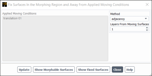
Select the method for creating the fixed condition as none, adjacency, or distance.
When none is selected, the fixed condition will be disabled.
The adjacency method will automatically fix any surfaces that are not adjacent to a zone containing moving surfaces.
When adjacency is selected for the method, you must define the Layers From Moving Surfaces. This value represents the the number of zones that will be used to create a transition region for passive mesh morphing in zones adjacent to the moving surface. For example, if you set the Layers From Moving Surfaces value to 1, only the zones immediately adjacent to the moving surface are allowed to be morphed, and all other zones will be fixed. If you set the value to 2, zones that are adjacent to the first layer are also allowed to be morphed, and so on.
The distance method allows you to define a specific distance from a moving surface that will undergo passive mesh morphing. You can set the distance by entering the distance value for Distance From Moving Surfaces.
After specifing the Method and method settings, you can click the Show Morphable Surfaces button to display the deformable surfaces. Within the graphics window, deformable surfaces will be shown in blue, while moving surfaces are displayed in green.
You can click the button to display the surfaces defined as fixed based on the distance specified away from moving surfaces. Fixed surfaces will be displayed in grey, while moving surfaces are displayed in green within the graphics window.
If the surfaces displayed for the fixed condition are satisfactory, you can click the button to save the fixed condition.
Note: This step is not applicable if you are defining Design Change settings within the Parameterize and Explore dialog box for geometry parameterization.
For each observable, specify its Weight in the optimization calculation. The weights are applied to the Target/Reference Change you specified in the Objectives tab. That is, if you have two observables that are each given a Weight equal to 1, Fluent will attempt to find an optimal design change that alters the observable values in proportion to their respective values for Target/Reference Change.
Note: Weights are only required if there are two or more objectives that do not have explicit target changes specified.
Note: This step is not applicable if you are defining Design Change settings within the Parameterize and Explore dialog box for geometry parameterization.
Specify the deformation parameters.
When using the Polynomials morphing method with the Standard constraint method, choose a Freeform Scaling Scheme and specify the Freeform Scaling Factor. This setting controls how the overall scaling factor for the design change magnitude is interpreted.
- Control-Point Spacing
The magnitude of the freeform deformation will be based on the control-point spacing. That is, a Freeform Scale Factor of
1.0leads a to maximum control point movement on the order of one sub-cell of the control volume. The sub-cell size is determined by a uniform sub-division of the morphed region based on the number of control points specified (Defining Region Conditions). A value of1.0is a reasonable default to preserve mesh quality during the morphing process.- Objective Reference Change
The magnitude of the freeform deformation will be based on the Target/Reference Change value in the Objectives tab. That is, for a single observable optimization with Freeform Scale Factor of
1.0, the design change computed will yield an expected change in the observable equal to the Target/Reference Change for the observable.
If you have disabled Auto-Select Smoothness in the Numerics tab, you can also specify a value for Smoothness of the deformed geometry. A lower value will allow locally sharper changes in the geometry, potentially at the expense of manufacturability. For details about this setting, see Design Tool Numerics.
If you used an input parameter as part of the setup of a deformation condition in the Design Conditions tab, the initial value will be displayed and is available for modification.
Click the button to verify that your constraining and/or deformation conditions are set up in such a way as to produce good results. A report will be printed in the console listing conflicts between multiple constraints / deformations applied on a single node (including the Design Conditions and the continuity constraint applied along the boundary of the morphing region). The conflicts are categorized as being either of type
Fatal(which indicates the solution is unlikely to converge or be desirable) orPossible(which may be allowable, depending on the details of the applied conditions).Click Calculate Design Change to compute the optimal design change. The Expected change for each observable will be reported in the Design Tool dialog box.
(optional) You can export the expected changes or displacements by clicking the button then selecting one of the following from the drop-down list:
Note: The Export Expected Changes... option is not available if you are using the Parameterize and Explore dialog box for geometry parameterization.
Click Export Expected Changes... to write to file the adjustment in the observable that is expected due to the change defined by the current settings.
Click Export Displacements... to write to file the optimal surface displacement field (overwriting any pre-existing file of the same name). An example of the format of the text file that is written (for a 3D mesh) is as follows:
                                        Line 1:
                                        n
                                        Lines 2 to n+1:
                                        x y z dx dy dz
This displacement field is for the calculated design change for the current mesh. If you plan to repeatedly create a series of iterations of a design (to gradually deform the mesh), you can also compare exported displacements to a reference mesh, set at an appropriate iteration. This is done using the Mesh History dialog box, as described in a later step.
The planned change to the geometry can be displayed in the graphics window by clicking the button and then using the Preview Morphing dialog box that opens to display the surfaces of interest. Note that you can use the buttons to easily select all the boundaries and/or the surfaces, and you can increase the Scale to accentuate the morphing preview or exported
.stl. When you click the button, the selected surfaces are displayed undeformed in white and deformed in green.Note that for 3D cases you can also use the Export STL... button to export the previewed mesh as an
.stlfile. This is useful for large cases, as it means you do not have to actually morph the mesh in order to have the previewed geometry available for use in other software packages.If you plan to repeatedly create a series of iterations of a design (to gradually deform the mesh), you can set the current mesh to be a reference mesh, and then at a later design iteration you can export the displacement field of the design compared to this reference mesh. This is different than using the button in the Design Export dialog box, as that button does not allow you to see the total displacements over multiple instances of mesh modification. To start this process, click the button to open the Mesh History dialog box.
Click the button to specify the current mesh as the one used for comparisons in the future. After it has been set, this button changes to , which can be used if you decide that the mesh from a later design iteration should instead be used as the reference mesh.
After you have modified the mesh (as described in the next step) one or more times, you can return to this dialog box; then, for the selected Surfaces, you can do the following:
Click the button to visualize the displacements in the graphics window. The reference mesh is displayed in green and the modified mesh is displayed in white.
Click to write to file the surface displacement field (overwriting any pre-existing file of the same name). An example of the format of the text file that is written (for a 3D mesh) is as follows:
                                        Line 1:
                                        n
                                        Lines 2 to n+1:
                                        x y z dx dy dz
Note: The following limitations apply to the use of the Mesh History dialog box:
The reference mesh can only be saved in a CFF case file (which is the default format).
Any operation that changes the node count (such as remeshing or adaption) is not supported.
Click the button in the group box to deform the boundary and interior mesh with the optimal design change. You should then examine the modified shape and mesh to determine if the results are satisfactory, using the usual commands for viewing the mesh in Ansys Fluent. When using the Direct Interpolation morphing method, it is recommended that you check the resulting mesh quality and verify that no boundary zones cross / penetrate themselves or other boundary zones. Note that the Direct Interpolation morphing method is not applicable if you are using the Parameterize and Explore dialog box for geometry parameterization.
If you determine that the change is unsatisfactory, you can click Revert to undo the mesh changes.
After modifying the mesh you can click the button to remesh the modified geometry, which can improve mesh quality and fix negative cell volumes. Remeshing can lead to a better design, especially for large geometry changes after modifying the mesh in the previous step. Remeshing is accomplished using the unified remeshing method in Fluent and uses the unified remeshing settings defined within the Dynamic Mesh task page (see Advanced Remeshing Settings Dialog Box). Upon clicking the button, deforming dynamic mesh zones are automatically created in the morphing region and when remeshing is complete, the dynamic mesh zones are deleted. Only tetrahedral and prism meshes for 3D cases and triangle meshes for 2D cases can be remeshed and all other types of meshes will not be affected by remeshing. Once the modified geometry has been remeshed, the new mesh can not be reverted and any previously defined reference meshes within the Mesh History dialog box will not be accessible due to changes in the mesh connection.
After the mesh has been modified according to the control settings, the original flow calculation can be restarted and converged with the modified geometry. Upon successful convergence, the observable value should now have changed by an amount similar to that reported when the Export Expected Changes... button was clicked prior to deforming the geometry. Note that observable values and the Export Expected Changes... button is not relevant when using the Parameterize and Explore dialog box for geometry parameterization.
For 3D cases, you have the option of exporting the boundary surfaces and/or
isosurfaces from your modified geometry as an .stl
file, for use in other software packages. Click the
button near the bottom of the
Design Change tab and then click the button in the Export dialog box that
opens. Finally, select the Surfaces of interest in the
dialog box that opens (Figure 48.22: The Export STL Dialog Box) and
them.
The adjoint solver provides a Gradient-Based Optimizer that can automatically create a series of iterations of a design for both shape optimization and turbulence model optimization. For shape optimization, the mesh will gradually deform to an optimal shape in order to meet multiple objectives at multiple operating conditions. For turbulence model optimization, the adjoint-method and machine learning are combined to tune turbulence model parameters (e.g GEKO coefficients), with the aim of reducing the difference between the flow solution of a RANS (e.g GEKO) simulation and the flow solution of a high-fidelity simulation or results from an experiment. Using a neural network, the gradient-based optimizer will build an augmented turbulence model by correlating flow features with turbulence model parameters.
The workflow of the optimizer is shown in Figure 48.23: Gradient-Based Optimizer Workflow. Note that this figure represents the optimizer workflow when two operating conditions and two observables have been defined. After the flow solution is calculated for a specified operating condition, the adjoint equations are solved for each individual observable in sequence. For example, if three observables and four operating conditions are defined, the optimizer worklow will resemble the following procedure:
Flow solution is calculated for operating condition 1
Adjoint equations are solved for observable 1
Adjoint equations are solved for observable 2
Adjoint equations are solved for observable 3
After the adjoint equations are solved for observable 3 for the first operating condition, the procedure will repeat for the next operating condition. When the flow solution and adjoint equations have been solved for all operating conditions and all observables, the design change will then be calculated followed by the design modification.
To prepare to use the Gradient-Based Optimizer, you will perform most of the usual steps outlined in Using the Adjoint Solver with the following exceptions:
It is not necessary to start with a converged flow solution; simply initializing the case file is sufficient.
It is not necessary to select a single observable in the Adjoint Observables dialog box, as you will be able to select multiple observables in a separate dialog box.
It is not necessary to initialize the adjoint solution and iterate to convergence using the Run Adjoint Calculation dialog box, as these actions will be performed in the Gradient-Based Optimizer dialog box.
For shape optimization, when setting up the Design Tool :
It is not necessary to export / import sensitivity data, as this will be handled automatically during optimization.
It is not necessary to specify the objectives for the observables in the Objectives tab of the Design Tool dialog box, as this will be done in the Gradient-Based Optimizer dialog box.
In the Design Change tab of the Design Tool dialog box, it is not necessary to take any action in the Workflow , Mesh, and Results group boxes.
Note: Setting up the Design Tool is only necessary for shape optimization. When using the Gradient-Based Optimizer for turbulence model optimization, optimization settings will be specified within the Turbulence Model Design Tool group box as outlined in Using the Turbulence Model Design Tool.
While the above steps are not necessary, you may yet want to perform them in order to verify that your settings are properly defined (for example, to ensure your design conditions are not conflicting for shape optimization) prior to using the optimizer.
For turbulence model optimization, the following additional steps are required prior to using the Gradient-Based Optimizer :
The GEKO turbulence model must be selected within the Viscous Model as outlined in Setting up the Generalized k-ω (GEKO) Model.
Adjoint Turbulence must be enabled within the Adjoint Solution Methods dialog box as outlined in Using the Adjoint Solution Methods Dialog Box.
Adjoint Observables specific to turbulence model optimization should be defined as outlined in Defining Observables for Turbulence Model Optimization.
Prior to configuring settings within the Turbulence Model Design Tool group box as outlined in Using the Turbulence Model Design Tool, it is recommended to plot sensitivity contours for the GEKO coefficients of interest (e.g Contours of Sensitivities... to Sensitivities to GEKO CSEP) to observe their influence on your RANS simulation. Selecting Design Variables for GEKO parameters with large sensitivity magnitudes will increase the controllability of tuning during optimization.
To start, you must define the settings for the flow solution and initialize it; if you want to optimize the design for multiple operating conditions, as part of this step you should create input parameters for the cell zone and boundary condition settings you would like to vary. Next, you must define the adjoint observables, methods, solver controls, monitors, and Design Tool (for shape optimization) or Turbulence Model Design Tool (for turbulence model optimization), noting the exceptions listed previously. Then you can open the Gradient-Based Optimizer dialog box by clicking in the Design ribbon tab ( Gradient-Based group box).
Design →
Gradient-Based → Gradient-Based
Optimizer...
The general procedure to use the Gradient-Based Optimizer is as follows:
Select the Optimizer Type from the Type drop-down list.
For shape optimization, select shape-opt .
For turbulence model optimization, select turb-model-opt.
Click the button to open the Adjoint Optimizer Observables dialog box. You can click the button to create and/or edit observables (as described in Defining Observables).
For shape optimization, you can select all of the relevant observables for your optimization problem in the Adjoint Optimizer Observables dialog box.
For turbulence model optimization, refer to Defining Observables for Turbulence Model Optimization to create and edit observables specific to turbulence model optimization. After defining the observables for your optimization problem, you can select all of the relevant observables in the Adjoint Optimizer Observables dialog box.
Select the Observable Evaluation method from the Method drop-down list. You have the following options:
When instantaneous is selected, the observable value will be evaluated as it's current instantaneous value at the end of the flow solver.
When averaged is selected, the observable will be evaluated as it's average value over a specified Sampling Interval. You can also set the Start after Iteration value to begin averaging the observable after a certain interval.
After you have selected the desired observables for your optimization problem and specified the Method for Observable Evaluation, click to close the Adjoint Optimizer Observables dialog box.
Click the button to open the Adjoint Optimizer Conditions dialog box.
Define the following:
- Number of Operating Conditions
This defines the number of possible operating conditions. Each operating condition is a set of simulation properties for which a flow solution will be calculated. As you increase this number, more rows will be added to the group box below, each with a unique No.. The Active? option must be enabled to calculate the flow for that operating condition.
- Number of Input Parameters
This defines the number of input parameters you would like to define for each operating condition. As you increase this number, more columns will be added to the group box below. You can select an input parameter from one of the top drop-down lists, and then define its value for each operating condition in the number-entry boxes below it.
When you have defined all the operating conditions, click , and close the Adjoint Optimizer Conditions dialog box.
Fill out the following columns for the table in the Objectives group box. Each row represents a unique combination of the active operating conditions and the selected observables defined in the previous steps.
- Goal
This determines how Fluent will attempt to change the value of the observable through the design change. You can specify a Target change in value; otherwise you can select None, in which case the observable will not be considered in computing the optimal design change, and the predicted change in observable value will not be reported.
- Step Size
When the Goal is a Target change in the observable for each design iteration, this field corresponds to the desired or initial change in the observable for each design iteration.
- Percentage?
Enabling this option specifies that the Step Size is a percentage of the value of the observable.
A target change of 5–10% is typically a good starting point, depending on the problem.
The Optimizer Settings group box allows you to view / set the following:
- Method
Specifies step size behavior during optimization. The optimization methods are as follows:
- fixed-step-size
The fixed step size method will advance the optimization based only on the user-specified Step Size, regardless of whether the observable values improve or worsen. For shape optimimization, the Step Size will only be reduced if the mesh quality requirement is not met, which is also true for the adaptive-step-size and line-search methods.
- adaptive-step-size
When using this method, Fluent automatically detects when a design iteration produces non-optimal results (compared to previous flow solutions), and reattempts the design using Objectives settings that are less aggressive. The process is as follows: the solution calculated for the initial design is considered optimal and written to disk; then the following two steps are repeated.
The design is revised based on the current Objectives settings.
The flow solution is calculated, and the results are compared to the optimal design solution:
If the values of all of the observables for all of the operating conditions improve or remain the same, the revised design solution is deemed the new optimal (and the files are overwritten), and the process returns to step 1.
If the value of any of the observables for any of the operating conditions worsens, the optimal design solution is restored, the Objectives settings are revised such that every Step Size is reduced by 50% going forward, a new design is generated, and the process returns to step 2.
- line-search
Note: The line-search option only supports optimization of a single Observable.
The line search method aims to find the optimal design change along the direction of the gradient to improve the value of the observable during each design iteration. During each design iteration, the flow solution, adjoint solution, and gradients are first computed. The case and data files are then written to disk as the baseline for the line search. The line-search then performs sub-iterations to find the optimal step size needed to improve the observable value. For each sub-iteration, the following steps are performed:
The case and data files are read and the step size is adjusted.
The design change is calculated.
The design is modified based on the design calculation.
The flow solution is calculated for the modified design.
The observable value is recorded.
Once the optimal step size is found, it is then used for the next design iteration and the above process is repeated.
Note that when the line-search method is selected, one design iteration will consist of one adjoint calculation and multiple flow calculations (typically in the range of 5-10). Alternatively, when the fixed-step-size or adaptive-step-size methods are selected, one design iteration will consist of one flow calculation and one adjoint calculation.
For shape optimization, if the adjoint convergence is poor or if the shape sensitivity distribution is not irregular, the line-search method may produce a much better solution compared to the adaptive-step-size and fixed-step-size methods.
When using the adaptive-step-size or line-search methods, note that:
The naming convention for the optimal design solution files is provided in a later step that describes how to set up autosaving.
You must ensure that you have sufficient disk space for the optimal design solution files.
You must not remove or rename the optimal design solution files during optimization.
You must ensure that the optimal design solution files are in the correct folder if you stop the optimization and then continue it.
If a problem occurs during optimization, you can either:
initialize the optimizer again: the current design solution files will be saved as the optimal if optimization continues, and the Curr. Design Iteration will be reset to 0 and the optimization history in the monitor plot will be lost.
reset it: the current design solution files will be saved as the optimal if optimization continues, but the Curr. Design Iteration will not be reset to 0 and the optimization history in the monitor plot will not be lost.
If you stop the optimizer, modify some settings, and then continue the calculation, note that your changed settings may be overwritten if the optimal design solution is restored during the first iteration.
- Curr. Design Iteration
This displays the current design iteration.
- No. of Design Iterations
This specifies the maximum number of design iterations that the optimizer will perform. A value in the range of 10–20 is typically appropriate, depending on the problem and settings. When using line-search as the optimization method, a value in the range of 4–10 is recommended.
- Convergence Criteria
This defines the criteria by which the design is considered converged. For every observable at every operating condition, the following are calculated during various points in the design iteration:
the expected change / initial value (when the design change is calculated)
the actual change / initial value (when the flow solution is calculated)
When either of the above are less than your specified Convergence Criteria for all observables at all operating conditions, the optimizer will stop iterating. If you want to continue the optimization, you can either reduce the convergence criteria or initialize/reset the optimizer.
- No. of Flow Iterations
This specifies the maximum number of iterations performed during the calculation of the flow solution. A starting value of 300 is typically appropriate, depending on the problem and settings.
- No. of Adjoint Iterations
This specifies the maximum number of iterations performed during the adjoint calculation. A starting value of 500 is typically appropriate, depending on the problem and settings. When using the blending stabilization strategy, the adjoint solver will stop early when the max iteration of the 2nd scheme has been reached. See Stabilization Strategies, Schemes, and Settings for details.
For turbulence model optimization:
Click the Design Region... button to open the Optimizer Design Region dialog box and specify the desired (see Defining the Design Region).
Click the Design Variables... button to open the Optimizer Design Variable Settings dialog box and specify the settings for your optimization problem. For detailed instructions on specifying these settings see Defining Optimizer Design Variable Settings.
For shape optimization:
Click the button if you need to set up or edit the settings in the Design Tool dialog box. Note that you do not need to perform all of the steps that are necessary when not using the Gradient-Based Optimizer, as described at the beginning of this section.
Specify the settings in the Mesh Quality group box.
By default, the cell volume and orthogonal quality (as defined in Mesh Quality) is computed at the start of every design iteration, before the flow solution is calculated; if the mesh violates your specified Min. Cell Volume and/or Min. Orthogonal Quality, the optimizer stops. Such a check is also performed immediately after each design change is calculated; if this check fails, Fluent reattempts the design using Objectives settings that are less aggressive, in the same manner as described previously for the adaptive-step-size option (regardless of whether that option is selected). This helps to ensure that your solution accuracy is not compromised by poor quality meshes. When the direct interpolation method is used, the mesh quality may deteriorate quickly at local regions, therefore the value will be reduced quickly. You may continue the optimization by readjusting the value, accordingly. When setting these minimums, you can click the button and enter values that are sufficiently lower then those printed in the console, so as not to reject a majority of the meshes generated during the optimization process. Note that it is recommended that you set the Min. Orthogonal Quality to a value greater than 0, in order to avoid left-handed faces.
The Smoothing option within the Post Morph group box is enabled by default. This will smooth the mesh at the end of the design iteration (after the mesh has morphed). You can enable the Remeshing option to remesh the geometry at the end of the design iteration (after the mesh has morphed) which can improve the mesh or fix negative cell volumes. Remeshing can lead to a better design, especially for large geometry changes after modifying the mesh. Only tetrahedral and prism meshes for 3D cases and triangle meshes for 2D cases can be remeshed and all other types of meshes will not be affected by remeshing. Additionally, any other remeshing limitations outlined in the Remeshing step of Shape Modification will also apply to shape optimization.
You can set up a monitor of the optimization history by clicking the button in the Calculation Activities group box.
The Adjoint Optimization History Monitor dialog box has the following controls:
- Plot During the Optimization
This option specifies whether plotting is performed for each design iteration.
- Observable Values
This option enables the plotting of observable values from the flow calculation. The data is represented by solid lines.
- Expected Observable Values
This option enables the plotting of expected observable values for the next design iteration. It is calculated by taking the current observable value and adding the expected change due to the mesh morphing (for shape optimization) or design variable tuning (for turbulence model optimization) in the current design iteration. The data is represented by dashed lines. If dashed and solid lines of the same color do not match well, that is a sign that the sensitivity is not accurate for that observable, and so you may need revise your setup (improve the convergence of the flow and/or adjoint solvers, reduce optimization values, and so on).
- Normalize
Enabling this option specifies that the plotted values are normalized based on the values at the first design iteration. This can be helpful for multi-objective optimization when the values for the observables are quite different.
- Plot All Optimization IDs
This option enables the plotting of data for all optimization IDs, that is, all of the rows of the table in the Objectives group box; otherwise, only a single optimization ID will be plotted.
- Optimization ID to be Plotted
This field specifies the individual optimization ID to be plotted, and is only available when the Plot All Optimization IDs option is disabled. The number you enter corresponds to the ID in the Objectives group box.
You can set up the automatic saving of files during optimization by clicking the button in the Calculation Activities group box. All of the files will be saved after the adjoint design calculation but before the morphing of the mesh (for shape optimization).
The Adjoint Optimizer Autosave dialog box has the following controls:
- File Name
This field specifies the root name for the files that are saved. It is suggested that you do not include an extension for the file name. If you include a folder, you must make sure that it is accessible.
- Save Case and Data Files (Every Design Iteration)
This group box allows you to specify settings for the autosaving of case and data files. Every (Designs) sets the frequency, in design iterations. The Max. Files Retained sets the limit after which the earliest existing files are overwritten by the latest.
The files are saved with the following names:
<auto_name>
-design-<des_iter>.cas.h5<auto_name>
-design-<des_iter>.dat.h5<auto_name>
-id-<optimization_id>.sens(only when you have defined multiple operating conditions and/or objectives)
where <auto_name> is the File Name , <des_iter> is a three-digit number corresponding to the design iteration, and <optimization_id> is a two-digit number corresponding to the ID in the Objectives group box.
- Save Optimal Case and Data Files
This group box provides the Save During the Optimization option; when enabled, a single set of optimal design solution files is saved and rewritten as necessary (as described previously in the step describing the adaptive-step-size option). The files are saved with the following names:
<auto_name>
-design-optimal.cas.h5<auto_name>
-design-optimal.dat.h5<auto_name>
-id-<optimization_id>-optimal.sens(only when you have defined multiple operating conditions and/or objectives)
where <auto_name> is the File Name and <optimization_id> is a two-digit number corresponding to the ID in the Objectives group box.
If you move the
.cas.h5/.dat.h5files to a different location, make sure to move the optimal.cas.h5/.dat.h5and.sensfiles (only when you have defined multiple operating conditions and/or objectives) along with it, and set up the proper File Name for the new location in order to continue the optimization. The optimal files are needed to restore the optimization. Otherwise, you can reset the optimizer and continue the optimization.Note that the Save During the Optimization option can only be disabled if you have disabled the adaptive-step-size option.
- Export STL Files (Every Design Iteration)
This group box allows you to set up the automatic exporting of
.stlfiles (for 3D cases only), for use in other software packages. Every (Designs) sets the frequency, in design iterations. The button opens the Export STL dialog box, where you can select Surfaces to specify the boundary surfaces / isosurfaces of interest.The files are saved as <auto_name>
-design-<des_iter>.stl, where <auto_name> is the File Name and <des_iter> is a three-digit number corresponding to the design iteration.
You can set up commands to be executed during optimization (such as postprocessing commands that export fields) by clicking the button in the Calculation Activities group box and using the Execute Commands Dialog Box that opens. For details, see Executing Commands During the Calculation. Note that once you have opened this dialog box from Gradient-Based Optimizer dialog box, the following selections become available in the When drop-down list:
- Adjoint Iteration
This specifies that execution of the command is based on the adjoint iteration. It is executed immediately before each adjoint advancement step.
- Design Iteration
This specifies that execution of the command is based on the design iteration when the keyword
;@is not entered after the command. The command will be executed after the design calculation and before any animation recording, both of which are before the morphing of the mesh.Commands can also be set to execute before or after specific calculations in the optimization process (see Figure 48.23: Gradient-Based Optimizer Workflow for details). The following keywords can be entered after typing in a command within the Execute Commands dialog box:
;@before-optimizationSpecifies the command to execute immediately before optimization begins
;@after-optimizationSpecifies the command to execute immediately after optimization is complete
;@before-flowSpecifies the command to execute immediately before the flow calculation.
;@after-flowSpecifies the command to execute immediately after solving the flow calculation.
;@before-adjointSpecifies the command to execute before the adjoint calculation.
;@after-adjointSpecifies the command to execute immediately after the adjoint calculation.
;@before-design-calculationSpecifies the command to execute immediately before calculating the design change.
;@after-design-calculationSpecifies the command to execute immediately after calculating the design change.
;@before-modifySpecifies the command to execute immediately before the design modification.
;@after-modifySpecifies the command to execute immediately after the design modification.
Note: If the keywords are not entered exactly as listed above, then the command will not be executed. Additionally, it is recommened to leave a space between the command and the
;@keyword.For example, the execute command
adjoint/observable/write yes
                                        out/adjoint-obs.monset ;@after-flow
will write the adjoint observable values to file immediately after the flow solution is calculated.
Note that unexpected behavior may result if the executed command changes settings for the adjoint calculation and/or gradient-based optimizer.
You can set up animations to be recorded during optimization by clicking the button in the Calculation Activities group box and using the Animation Definition Dialog Box that opens. For details, see Creating an Animation Definition. Note that once you have opened this dialog box from Gradient-Based Optimizer dialog box, the following selection becomes available in the drop-down list next to the Record after every field:
- design-iteration
This specifies that the recording is based on the design iteration. It is recorded after the design calculation and the execution of any commands, and before the morphing of the mesh (for shape optimization).
For details on playing, saving, and/or reading the resulting animation, see Animating the Solution.
For shape optimization:
Click the button in the Calculation group box of the Gradient-Based Optimizer dialog box.
For turbulence model optimization:
You can click the button in the Calculation group box of the Gradient-Based Optimizer dialog box if you want to clear the optimization history, or switch between shape optimization and turbulence model optimization.
Click the button to start the design iterations. After clicking the button the Optimize dialog box will open, which can be used to stop the optimization at the end of the current design iteration or stop the optimization immediately by clicking the button or the button, respectively.
The optimizer will proceed until one of the following conditions is met:
the Convergence Criteria is met for all of the observables
the No. of Design Iterations is reached for this optimizer run
the mesh quality requirements cannot be met (for shape optimization)
you interrupt the calculation
an error occurs
If you want to continue to optimize the design with revised settings for the observables, operating conditions, objectives, and/or the adaptive-step-size option, it is recommended that you either the optimizer again or it: the current design solution files will be saved as the optimal if optimization continues, and (for ) the Curr. Design Iteration will be reset to 0 and the optimization history in the monitor plot will be lost.
When the optimization is complete, you can click the button to print a report of the results for each design iteration in the console, including the observable values, the expected changes, whether the flow and adjoint calculations converged, and the mesh quality metrics.
For turbulence model optimization, after optimizing the design variables in offline mode (e.g Field Inversion), continue to the Offline training procedure outlined in Offline Mode Optimization. For online mode optimization, continue to Managing Trained Turbulence Models if you would like to export the neural network turbulence model.
When using the Gradient-Based Optimizer, note the following:
It is a good practice to initially run the optimizer for one design iteration, in order to check if the settings are proper.
The resulting design will be highly affected by whether or not the flow solver and/or adjoint solver reach convergence. Auto-adjust controls and blend stabilization strategies are recommended for convergence of the adjoint solver.
You may want to perform a first round of optimization using lower accuracy settings, and then switch to higher accuracy settings as you approach the optimal solution. For the first round you could consider using the following:
settings (for example, in the Solution Method task page) that help flow convergence and/or reduce the residual oscillation
a coarser mesh (for shape optimization)
If you change the settings during the optimization (which can change an observable value), you should make sure to initialize or reset, so that the optimizer considers the current solution to be optimal and starts the optimization from the current solution; otherwise, the changed observable value may be worse than in previous calculations, and if the adaptive-step-size option is enabled, Fluent will restore the saved optimal solution and continue, which will undo your settings changes.
Adjoint-based turbulence model optimization is supported by the adjoint solver within the Gradient-Based Optimizer. Turbulence model optimization utilizes the adjoint method and machine learning to build an augmented turbulence model that correlates flow features with turbulence model parameters (e.g CSEP or CMIX). The goal of turbulence model optimization is to reduce the difference between the computed results of a GEKO simulation and the results computed by a high-fidelity simulation or experimental data.
Prior to using the Gradient-Based Optimizer for turbulence model optimization you must perform the following:
Enable the GEKO turbulence model within the Viscous Model (see Setting up the Generalized k-ω (GEKO) Model).
Enable Adjoint Turbulence within the Adjoint Solution Methods dialog box (see Using the Adjoint Solution Methods Dialog Box).
Create and edit the adjoint Observables specific to turbulence model optimization as outlined in Defining Observables for Turbulence Model Optimization.
Specify all relevant settings for your optimization problem within the Gradient-Based Optimizer dialog box as outlined in Using the Gradient-Based Optimizer.
Prior to defining optimization settings outlined in Defining Optimizer Design Variable Settings, it is recommended to plot sensitivity contours for the GEKO coefficients of interest (e.g Contours of Sensitivities... to Sensitivities to GEKO CSEP) to observe their influence on your RANS simulation (e.g GEKO simulation). Selecting Design Variables for GEKO parameters with large sensitivity magnitudes will increase the controllability of tuning during optimization.
Design →
Gradient-Based → Gradient-Based
Optimizer...
Turbulence model optimization can be performed using one of two strategies referred to as offline mode optimization and online mode optimization.
Note: Online mode optimization is currently the recommended optimization method.
In online mode, the Design Variables are a specific function of flow Input Features in the form of a Neural Network. The neural network model has a topology defined within Optimizer Design Variable Settings and during optimization the design variables are optimized directly. After optimization, the correlation between the optimized design variables and flow input features are known and do not need to be learned through Offline Training. Refer to Online Mode Optimization for the online mode optimization workflow.
In offline mode, the Design Variables are represented as varying coefficient fields and are not a function of flow Input Features .To compute the optimal design variable fields, field inversion is performed using gradient-based optimization. When optimization is complete, the optimized solution is generalized through Offline Training which uses machine learning to create the correlation between the optimized Design Variable field and flow Input Features . Refer to Offline Mode Optimization for the offline mode optimization workflow.
When deciding whether to use offline mode or online mode optimization, consider the following advantages and disadvantages of both methods:
For online mode optimization it is not necessary to define Offline Training settings or train the Neural Network after optimization, which simplifies the workflow. Optimization is model consistent as well because the neural network model is integrated within the entire optimization process. Additionally if the optimization results are acceptable, the optimized model will be numerically stable and demonstrate improved performance when compared to the original flow solution.
The disadvantage of online mode is that Neural Network settings must be defined prior to optimization, and therefore training settings (which are defined in Offline Training) can not be customized after optimization.
For offline mode optimization, the Neural Network model is not used during optimization (field inversion) and there are no pre-defined neural network settings that could restrict the optimizer from solving for the optimal Design Variables. This allows for more extensive optimization and the flexibility for the optimizer to solve for all possible solutions. Settings for Offline Training are specified after the design variables have been optimized, and various training settings can be explored and customized after optimization.
The disadvantage of offline mode is that the Models being used for optimization and training are not consistent, which can lead to some optimization information being lost during Offline Training . When training is complete and when the trained turbulence model is hooked to the flow solver, the results may deteriorate and the trained model may be numerically unstable.
Offline and online mode optimization methods can also be used together to find the appropriate Neural Network settings prior to training the model. This can be done by initially performing offline mode optimization (including Offline Training) as a pre-training step to find the appropriate neural network Model settings (e.g flow Input Features and Neural Network Topology) for your optimization problem. Once the appropriate neural network settings have been configured, you can perform the online mode optimization workflow using the appropriate neural network settings.
For performing turbulence model optimization in online mode, the general procedure is as follows:
Online Mode Optimization:
Define the Design Region (see Defining the Design Region ).
See Defining Design Variables for Optimization for information on defining the following:
Select the design variables to be optimized.
(optional) Initialize the design variable field and set the design variable .
Select Neural Network from the Type drop-down list for the optimization Model, which will specify the design variables as a function of flow Input Features (see Defining the Model for Design Variables ).
Configure the neural network settings (see Defining Neural Network Model Settings).
Click the button so that
adjoint-modelupdates the GEKO model settings during optimization (see Defining the Model for Design Variables ).Click the button to close the Optimizer Design Variable Settings dialog box.
Within the Gradient-Based Optimizer dialog box, perform the optimization procedure as outlined in Using the Gradient-Based Optimizer.
(optional) Export the trained turbulence model to be applied on a similar case (see Managing Trained Turbulence Models).
For performing turbulence model optimization in offline mode, the general procedure is as follows:
Field Inversion:
Define the Design Region (see Defining the Design Region ).
See Defining Design Variables for Optimization for information on defining the following:
Select the design variables to be optimized.
(optional) Initialize the design variable field and set the design variable .
See Defining the Model for Design Variables for information on defining the following:
Use the None design function Type for the optimization Model which will specify the design variables as a varying coefficient field to be optimized using field inversion.
Click the button so that
adjoint-modelupdates the GEKO model settings during optimization.
Click the button to close the Optimizer Design Variable Settings dialog box.
Within the Gradient-Based Optimizer dialog box, perform the optimization procedure outlined in Using the Gradient-Based Optimizer.
When optimization is complete, verify the results by plotting sensitivity contours for the optimized design variable field (e.g Contours of Sensitivities... to Adjoint GEKO CSEP). In general, the change to the GEKO coefficients will be very local near the wall boundary and wake region.
Offline Training:
After checking the distribution of the optimized design variable field, click the button within the Gradient-Based Optimizer to reopen the Optimizer Design Variable Settings dialog box.
Select Neural Network from the Type drop-down list for the optimization Model, which will specify the design variables as a function of flow Input Features (see Defining the Model for Design Variables ).
Specify the neural network Settings (see Defining Neural Network Model Settings).
Perform the procedure for training the neural network turbulence model outlined in Defining Offline Training Settings, which includes:
Configuring Offline training settings.
(optional) Managing training data used for training the model.
Training the neural network model.
Verify the training results and apply the trained trained turbulence model (see Verifying the Trained Turbulence Model).
(optional) Export the trained turbulence model to be applied on a similar case (see Managing Trained Turbulence Models).
Prior to defining Optimizer Design Variable Settings , click the Design Region... button within the Turbulence Model Design Tool group box to open the Optimizer Design Region dialog box.
Specify the desired for your optimization problem.
In general, regions near walls and the wake region are of interest.
After selecting the Design Zones, click to close the Optimizer Design Region dialog box.
This section defines the various Optimizer Design Variable Settings and provides instruction on how to define them for both offline and online mode optimization strategies.
Click the Design Variables... button within the Gradient-Based Optimizer dialog box to open the Optimizer Design Variable Settings dialog box.
When choosing Design Variables to optimize, consider the following:
You can click the Options... button to open the Design Variable Options dialog box which allows you to turn on the option.
This option will enable the turbulence source coefficient design variables (TKE and Omega). When enabled,
and
will be added as source terms to the transport equations for turbulence kinetic energy (
) and specific dissipation rate (
).
Where,
is the TKE Source Coefficient
And,
is the Omega Source Coefficient
You can plot contours of Machine Learning Tke Coefficient and Machine Learning Omega Coefficient (both in the Turbulence... category) to observe their influence.
Sensitivities for GEKO coefficients of interest can be plotted to observe their influence (for example, Sensitivities to GEKO CSEP in the Sensitivities... category). Selecting Design Variables for GEKO parameters with large sensitivity magnitudes will increase the controllability of tuning during optimization.
In general, selecting TKE Source Coefficient as the design variable is recommended for the following reasons:
More tuning flexibility compared to GEKO coefficients such as CMIX, which can be deactivated by the blending function.
Works independently along with GEKO coefficients with the highest sensitivities.
If you choose not use TKE Source Coefficient, generally CSEP and CMIX are the GEKO coefficients of interest. However, note that when optimizing CMIX for a bluff body problem, you may need to fix the blending function as the built-in blending function may deactivate CMIX in the wake region
Refer to the definitions of the GEKO coefficients in section Generalized k-ω (GEKO) Model of the theory guide to see if they are physically relevant.
You can click the Limits... button to open the Set Design Variable Limits dialog box and specify the upper and lower bounds of the design variables during optimization.
For bluff body problems and when Adjoint GEKO CMIX is selected from the list of Design Variables, you may need to increase the range so that CMIX can mimic the mixing effect of large unsteady vortex shedding. Too large of a limit however may break the calibration of basic cases.
After specifying the Design Variable Limits, click to close the Set Design Variable Limits dialog box.
You can click the Initialize button to initialize the field for the selected Design Variables with the default Fluent values.
Note that when the blending function is selected from the list of Design Variables , Adjoint GEKO BF will be initialized with the blending-function that is built into the GEKO settings by default. The built-in blending function is dependent on the flow state and therefore it is necessary to converge the flow solver prior to initializing Adjoint GEKO BF .
From the Type drop-down list of the Model group box, you can select the design function that will be used for optimization.
For optimizing the Design Variables in offline mode, choose None for the design function. This will specify the Design Variables as a field that will be optimized using gradient-based optimization (Field Inversion).
When using None as the optimization Model you can enable the Smooth Sensitivities option which generally helps to improve optimization by adding regularization to the updated sensitivity field.
For offline training and online mode optimization, select Neural Network for the design function Type. This will specify the Design Variables as a function of flow Input Features in the form of a neural network.
During optimization for both optimization methods, the
adjoint-model is automatically hooked
to the relevant GEKO coefficients within the
Viscous Model. The
adjoint-model can be unhooked at
anytime to use the default GEKO settings by
clicking the button.
Alternatively, you can click the button to apply the
adjoint-model to the
GEKO coefficients and overwrite the default
GEKO coefficients using the trained model
during optimization.
The following Neural Network settings should be defined when using Offline Training or online mode optimization:
- Activation Function
This specifies the nonlinear activation function of nodes within the hidden layers of the neural network during optimization.
Note: Although various Activation Functions are provided for the Neural Network, the Activation Function does not appear to have a significant affect on optimization or training results.
- tanh
The tanh activation function is a sigmoidal hyperbolic tangent function with an output range of
-1to1.
- Softsign
The Softsign activation function has an output range of
-1to1and is similar to the tanh function, where tanh grows exponentially and Softsign grows polynomially. Softsign has the advantage over tanh in that Softsign is less likely to become saturated when there are large or small inputs to the function. The Softsign function also has a zero-centered range which increases the learning effectiveness. However when the input is zero, nodes will become inactive which can cause gradient saturation.
- ReLu
The ReLu (Rectified Linear Unit) activation function is an unbounded activation function that is linear in the positive dimension, but zero in the negative dimension.
The advantages of using the ReLu activation function include:
The activation of nodes in the network is minimal. In a randomly initialized network, only about 50% of hidden nodes are activated (have a non-zero output).
The gradient propagation is improved when compared to bounded sigmoidal activation functions (e.g tanh and Softsign) that can saturate in both directions causing gradient propagation to stop completely throughout all nodes in the network.
Computation of the ReLu activation function is more efficient compared to sigmoidal activation functions.
The disadvantage of using the ReLu activation function is that nodes in the network can be pushed into an inactive state for all inputs which stops the propagation of the gradient through the network. This is known as the vanishing gradient gradient problem and usually arises when the Learning Rate is set too high. This problem can be avoided by decreasing the Learning Rate, or by using the Leaky-ReLU activation function. However note that the neural network performance is reduced when using the Leaky-ReLU activation function.
- Leaky-ReLu
The Leaky-ReLU activation function is a linear variant of the ReLu activation function that outputs small positive gradient values at inactive nodes. The Leaky-ReLu function can be used as an alternative to the ReLu activation function if there is no gradient flowing backward through the nodes or if a large number of nodes in the network are inactive when using the ReLu activation function.
- Neural Network Topology
Defines the number of hidden layers in the neural network and the number of nodes in each hidden layer. By default, the neural network has three hidden layers consisting of
24,16, and8nodes for the first, second, and third layer, respectively. The input layer consists of the selected Input Features and the output layer outputs the Design Variables. A large neural network topology will be able to build a better correlation between Input Features (input) and Design Variables (output). However, large neural network topologies can be computationally expensive and may not be easy to generalize for use in other cases. A neural network topology that is too small may have more difficulty correlating the Input Features (input) and Design Variables (output).- Input Features
Selecting appropriate flow Input Features for your specific optimization problem is crucial for creating a succesful neural network model. By default, eight flow input features are available under the Input Features list, which have been carefully chosen based on the following physical principles:
Galilean invariance
Rotational invariance
Non-dimensional
Scaled
The following equations define the strain and rotation terms used to derive the invariant input features:
With,
(48–59)
(48–60)
The default flow input features are defined as follows:
Note: The Turbulent Reynolds Number (Scaled) and Turbulent Viscosity Ratio (Scaled) input features are only appropriate for low Reynolds number flows or for differentiating the boundary layer region with other regions.
- Non-Equilibrium Parameter
(48–61)
Where
is the specific dissipation rate.
Output range: [-1,3]
- Second Invariant
(48–62)
Where,
(48–63)
And,
(48–64)
Due to non-dimensionalization,
(48–65)
Output range: [0,1]
- Third Invariant
(48–66)
Where,
(48–67)
Output range: [0,1]
- Fourth Invariant
(48–68)
Where,
(48–69)
Output range: [0,1]
- Fifth Invariant
(48–70)
Where,
(48–71)
Output range: [0,1]
- Length Ratio
(48–72)
Where
and
are the turbulence kinetic energy and position in the y-direction respectively.
Output range: [0,2]
- Turbulent Reynolds Number (Scaled)
(48–73)
Where
is the molecular viscosity.
Output range: [0,2]
- Turbulent Viscosity Ratio (Scaled)
(48–74)
Where
is the turbulent viscosity ratio.
Output range: [0,2]
Flow input features that are not contained in the above list can be created by defining an Expression, and up to six expressions are allowed.
When optimization is complete, all input features can be plotted as Contours of Sensitivities... to the selected features (e.g Contours of Sensitivities... to Non-Equilibrium Parameter).
For specific cases and when performing online mode optimization, you can deselect all Input Features and enter
()for the Neural Network Topology, to use no hidden layers. This will specify the design variables as a constant field and the neural network model will be reduced to optimize the design variables as a global constant.
During training, the neural network will learn the correlation between the optimal Design Variable field and flow Input Features to produce a generalized optimal solution. Note that offline training should only be performed after performing offline mode optimization (Field Inversion). The procedure for Offline training is as follows:
Specify the Neural Network settings as outlined in Defining Neural Network Model Settings .
Define the following Offline Training settings:
- Maximum Epochs
Defines the maximum number of cycles ran through the full training data set.
- Mini Batch Size
Specifies the number of data samples (number of cells) used for correcting the neural network each time during the training process. The mini batch size should not be too large so the gradient can have some noise to escape from the local minimum or saddle points. The mini batch size should also not be too small as to approximate the full neural network gradient. A small mini batch size can be computationally expensive as well. A mini batch size between
10to1000should be appropriate for most cases.- Learning Rate
Defines the amount the neural network model adjusts in response to error after each iteration. A large learning rate value will increase the speed of the learning process, however it may lead to oscillation and divergence.
- Initialize Neural Network
When enabled, this will initialize the neural network model with random values during Offline Training. When disabled, training will continue on the existing model if there is any present.
Click the Manage Data... button to open the Manage Training Data dialog box.
The Manage Training Data dialog box allows you to use training data (which contain selected flow Input Features and Design Variables) from a different case or multiple different cases to train the neural network model for your current case. Training data can be exported as a
.tdatfile from your current case by clicking the button. Alternatively, you can import multiple.tdatfiles from different cases by clicking the button. If Include Current Data is enabled, training will be based on any existing training data from your current case as well as any imported training data that is selected from the Training Data Files list. If Include Current Data is disabled, then training will be based only on imported training data.Clicking the button will begin training the Neural Network model. Training is parallelized and training information is printed to the console. Statistics about the training data (e.g mean, covariances, and correlations) will be printed to the console as well. If the value for the flow input feature correlation printed to the console is close to
1or-1then the relevant flow input features are redundant and can be removed. Additionally during training, the optimization history will be plotted in the graphics window.
The following outlines the procedure for verifying the trained turbulence model created during Offline training :
When training is complete, you can compare the training results to the original sensitivity field by plotting sensitivity contours for the trained Design Variables (e.g Contours of Sensitivities... to Adjoint GEKO CSEP (Trained)). If the difference between the original and trained sensitivity field distributions are large, then you should continue training the model.
If the results produced from Offline training are acceptable, click the button to apply the augmented turbulence model to the Fluent turbulence model and update the Design Variables. Once the trained Design Variables have been applied they will no longer be accesible and the neural network model will be used to overwrite the GEKO model coefficients during the flow calculation.
Rerun the flow solution using the augmented turbulence model and analyze it's improvement from the original solution. Note that when the neural network model is used as the turbulence model during the flow calculation, the console will report that the turbulence model coefficients (e.g GEKO coefficients) are being updated using the neural network model.
Within the Management group box you can export
(from your current case) or import (from a different case), a trained
turbulence model as a scheme file (.scm).
If the flow solution produced using a trained turbulence model (created on your current case) is satisfactory, the trained model can be exported as a scheme file by clicking the button to be used on a different case with similar flow physics.
To use a turbulence model (trained on a different case with similar flow physics) on your current case, you can import the scheme file of the trained model by clicking the button.
Once the trained turbulence model has been imported into your current case, you can simply click the button, then run the flow solver using the trained turbulence model.
For Offline training, trained models from a different case (deployment case) can be imported to continue training the neural network of your current case (training case).
Note that data driven turbulence model tuning can be viewed as an advanced interpolation from the training condition to the deployment condition. Therefore the flow conditions and physics of the deployment case should be similar to the training case. If the deployment case and training case have different flow conditions and physics, the trained turbulence model may not be applicable, and the performance can deteriorate.
Additionally, you can click the button to delete all the existing information for your current model.


