


Boundary profiles are used to specify flow conditions on a boundary zone of the solution domain. For example, they can be used to prescribe a velocity field on an inlet plane. For information on boundary profiles, see Profiles. For information about transient profiles, see Transient Cell Zone and Boundary Conditions.
Profiles can also can also be used in expressions. Refer to Profiles for additional information.
For additional information, see the following sections:
To read the boundary profile files, open the Select File dialog box by selecting the File/Read/Profile... ribbon tab item.
![]() File → Read → Profile...
File → Read → Profile...
This opens the Select File dialog box so that you can read a boundary
profile with the standard extension .prof or a transient profile in
tabular format with the standard extension .ttab.
CSV profiles are also supported, see CSV Profiles for additional information. If a profile in the
file has the same name as an existing profile, the old profile will be overwritten.
Note: The maximum number of profiles that can be read into a single Fluent session is 50.
You can also create a profile file from the conditions on a specified boundary or surface. For example, you can create a profile file from the outlet conditions of one case. Then you can read that profile into another case and use the outlet profile data as the inlet conditions for the new case.
To write a profile file, use the Write Profile Dialog Box (Figure 3.4: The Write Profile Dialog Box).
![]() File → Write → Profile...
File → Write → Profile...
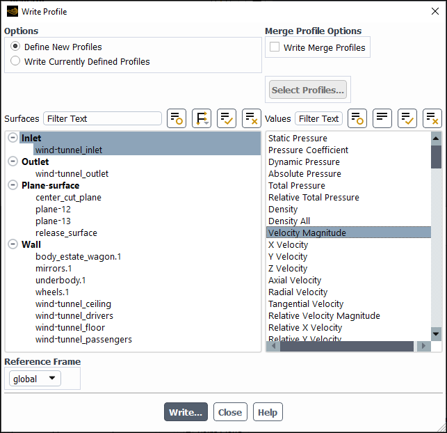
Retain the default option of Define New Profiles.
Select the surface(s) where you want data extracted for the profile(s) in the Surfaces list.
Choose the variable(s) for which you want to create profiles in the Values list.
Optionally select Write Merge Profiles. This writes a .csv file with the selected surfaces consolidated into one set of data points. Note that this option is only available if you have selected 2 or more surfaces.
Select the desired Reference Frame from the drop-down list that will be used for creating this profile.
Click Write... and specify the profile file name in the resulting Select File dialog box.
Ansys Fluent saves the mesh coordinates of the data points for the selected surface(s) and the values of the selected variables at those positions. When you read the profile file back into Fluent, you can select the profile values from the relevant drop-down lists in the boundary condition dialog boxes. The names of the profile values in the drop-down lists will consist of the surface name and the particular variable.
Select the Write Currently Defined Profiles option:
if you have made any modifications to the boundary profiles since you read them in (for example, if you reoriented an existing profile to create a new one).
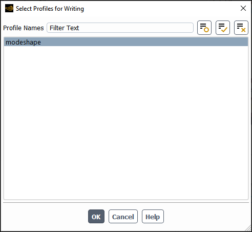
if you want to store one or more of the profiles associated with the current case file in a separate file. Note that you must click to select the specific profiles that you want written.
Click to open the Select Profiles for Writing box. This allows you pick the individual profiles that you want written.
Click to confirm the profile selection.
Click Write... and specify the file name in the resulting Select File dialog box. This file can be read back into Fluent whenever you want to use the profile(s) again.
Note:
Transformation of point profiles is only available for Cartesian reference frames. Cylindrical and other reference frame systems are not supported.
Scalar point field profiles do not require transformation to a local reference frame.
Transformation of vector point field profiles (for example, point velocities, acceleration) into local reference frames is not supported.
With Turbo Models enabled, you have the option to write circumferential-averaged profiles. Circumferential-averaged profiles are available for flow variables on various surfaces including inlet, outlet, interfaces, planes, iso-surfaces, and iso-clips. The determination of the profile type (radial or axial) is internally based on the specific type of machine.
To write a circumferential-average profile, perform the following steps:
Enable Turbo Models from the ribbon.
 Domain → Turbomachinery
→ Turbo Models
Domain → Turbomachinery
→ Turbo Models
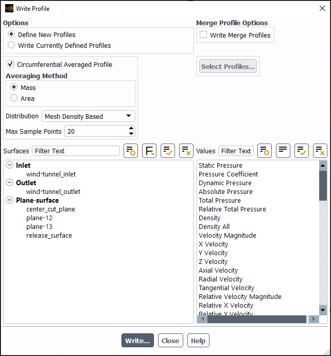
On the Write Profile dialog box, select Circumferential Averaged Profile to reveal additional settings. In most cases, the default settings should be sufficient.
Under Averaging Method, select Mass or Area.
Distribution determines how the averaged values for the profile pitch-wise bands are created. The distribution of bands can either be Mesh Density Based or Equal Distance Based.
Max Sample Points specifies the maximum number of bands that are created for sampling.
Select the Surfaces and Values to be included in the profile. If you select
X Velocity,Y Velocity, orZ Velocitythen Fluent automatically converts them into cylindrical coordinates so that extracted circumferential averaged velocity profile is always written in cylindrical components.Click Write... to generate the profile in
.csvor legacy.profformat. Note the main difference between the two formats is the.csvformat contains additional information in the file header.
You can also access this feature by using the following console command and following the prompts:
file/write-circumferential-averaged-profile