


Solution output is written to the:
Output file (Jobname.out)
Results file (Jobname.rst, Jobname.rth, or Jobname.rmg)
Program database (Jobname.db)
The output file is viewable via the GUI. The database and results file data can be postprocessed.
The following solution-output topics are available:
The output file contains the nodal degree-of-freedom solution, nodal and reaction loads, and the element solutions, depending on the OUTPR settings.
The element solutions are the solution values at the integration points or centroid. They are controlled by KEYOPTs in certain elements.
The results file contains data for all requested (OUTRES) solutions, or load steps. In POST1, SET identifies the load step that you intend to postprocess.
Results items for area and volume elements are generally retrieved from the database via standard results-output commands (such as PRNSOL, PLNSOL, PRESOL, and PLESOL).
The labels on these commands correspond to the labels shown in the input and output description tables for each element. For example, postprocessing the stress in the material x direction (typically labeled SX) is identified as item S and component X on the postprocessing commands. Coordinate locations XC, YC, ZC are identified as item CENT and component X, Y, or Z.
Only items shown both on the given results command and in the element input/output tables are available for use with that command. (An exception is EPTO, the total strain, which is available for all structural solid and shell elements even though it is not shown in the output description tables for those elements.)
Generic labels do not exist for some results data, such as integration point data, all derived data for structural line elements (such as spars, beams, and pipes) and contact elements, all derived data for thermal line elements, and layer data for layered elements. Instead, a sequence number identifies those items.
The element output items (and their definitions) are shown along with the element type description. Not all of the items shown in the output table will appear at all times for the element. Normally, items not appearing are either not applicable to the solution or have all zero results and are suppressed to save space. However, except for the coupled-field elements PLANE222, PLANE223, SOLID225, SOLID226, and SOLID227, coupled-field forces appear if they are computed to be zero. The output is, in some cases, dependent on the input. For example, for thermal elements accepting either surface convection (CONV) or nodal heat flux (HFLUX), the output will be either in terms of convection or heat flux. Most of the output items shown appear in the element solution listing. Some items do not appear in the solution listing but are written to the results file.
Most elements have two tables which describe the output data and ways to access that data for the element. The tables are the "Element Output Definitions" table and the "Item and Sequence Numbers" tables used for accessing data via ETABLE and ESOL.
Stresses and strains are two primary element solution quantities in structural elements used for stress analysis. Current-technology elements output Cauchy stresses, and logarithmic strains in large deflection analysis (NLGEOM,ON) or engineering strains in a small-deflection analysis (NLGEOM,OFF). Stresses and strains are directly evaluated at element integrations points, and may be extrapolated to element nodes or averaged at element centroid for output. Generalized stresses and strains, such as linearized stresses, forces, moments, and curvature changes, are available in beam, pipe, elbow, and shell elements.
The following element-solution topics are available:
- 3.2.3.1. The Element Output Definitions Table
- 3.2.3.2. The Item and Sequence Number Table
- 3.2.3.3. Surface Loads
- 3.2.3.4. Integration Point Solution (Output Listing Only)
- 3.2.3.5. Centroidal Solution (Output Listing Only)
- 3.2.3.6. Surface Solution
- 3.2.3.7. Element Nodal Solution
- 3.2.3.8. Element Nodal Loads
- 3.2.3.9. Nonlinear Solutions
- 3.2.3.10. 2D and Axisymmetric Solutions
- 3.2.3.11. Member Force Solution
- 3.2.3.12. Failure Criteria
- 3.2.3.13. Linearized Stresses
The first table, "Element Output Definitions," describes possible output for the element. In addition, this table outlines which data are available for solution printout (Jobname.out and/or display to the terminal), and which data are available on the results file (Jobname.rst, Jobname.rth, Jobname.rmg, etc.). Only the data which you request with the solution commands (OUTPR and OUTRES) are included in printout and on the results file, respectively.
As an added convenience, items in the table which are available via the Component Name method of ETABLE are identified by special notation (:) included in the output label. ( See The General Postprocessor (POST1) in the Basic Analysis Guide for more information.) The label portion before the colon corresponds to the Item field on ETABLE, and the portion after the colon corresponds to the Comp field. For example, S:EQV is defined as equivalent stress, and command for accessing the data is:
| ETABLE,ABC,S,EQV |
where ABC is a user-defined label for future identification on listings and displays. Other data having labels without colons can be accessed through the Sequence Number method, discussed with the "Item and Sequence Number" tables below.
In some cases there is more than one label which can be used after the colon, in which case they are listed and separated by commas. The Definition column defines each label and, in some instances, also lists the label used on the printout, if different. The O column indicates those items which are written to the output window and/or the output file. The R column indicates items which are written to the results file and which can be obtained in postprocessing; if an item is not marked in the R column, it cannot be stored in the "element table."
Many elements also have a table, or set of tables, that list the Item and sequence number required for data access using the Sequence Number method of ETABLE. (See The General Postprocessor (POST1) in the Basic Analysis Guide for an example.)
The number of columns in each table and the number of tables per element vary depending on the type of data available and the number of locations on the element where data was calculated.
See Table 182.2: PLANE182 Item and Sequence Numbers for a sample item and sequence number table. Items listed as SMISC refer to summable miscellaneous items, while NMISC refers to non-summable miscellaneous items.
Pressure output for structural elements shows the input pressures expanded to the element's full linearly or bilinearly varying load capability.
See SF, SFE, and SFBEAM for pressure input. Beam elements which allow an offset from the node on SFBEAM an have additional output labeled OFFST.
To save space, pressure output is often omitted when values are zero. Similarly, other surface load items (such as convection (CONV) and heat flux (HFLUX)), and body load input items (such as temperature (TEMP), fluence (FLUE), and heat generation (HGEN)), are often omitted when the values are zero (or, for temperatures, when the T-TREF values are zero).
To save space, surface output is often omitted when all values are zero.
For output of ocean-loading information on supported element types, see OCTYPE and OCDATA.
Integration-point output is available in the output listing with most current-technology elements. The location of the integration point is updated if large deflections are used.
See the element descriptions in the Mechanical APDL Theory Reference for information about integration-point locations and output. You can also issue ERESX to request integration-point data to be written as nodal data on the results file.
Output (such as stress, strain, and temperature) in the output listing is given at the centroid (or near center) of certain elements. The location of the centroid is updated if large deflections are used.
The output quantities are calculated as the average of the integration point values. The component output directions for vector quantities correspond to the input material directions which, in turn, are a function of the element coordinate system. For example, the SX stress is in the same direction as EX.
In postprocessing, ETABLE can calculate the centroidal solution of each element from its nodal values.
Surface output is available in the output on certain free surfaces of solid elements. A free surface is a surface not connected to any other element and not having any degree-of-freedom constraint or nodal-force load on the surface.
|
Surface Output Limitations The following limitations apply to surface output: |
The surface output is automatically suppressed if the element has nonlinear material properties. Surface calculations are of the same accuracy as the displacement calculations. Values are not extrapolated to the surface from the integration points but are calculated from the nodal displacements, face load, and the material property relationships. Transverse surface shear stresses are assumed to be zero. The surface normal stress is set equal to the surface pressure. Surface output should not be requested on condensed faces or on the zero-radius face (center line) of an axisymmetric model.
For 3D solid elements, the face coordinate system has the x-axis in the same general direction as the first two nodes of the face, as defined with pressure loading. The exact direction of the x-axis is on the line connecting the midside nodes or midpoints of the two opposite edges. The y-axis is normal to the x-axis, in the plane of the face.
The following table lists output available via ETABLE using
the Sequence Number method (Item = SURF). See the
appropriate table in the individual element descriptions for definitions of the
output quantities.
Table 3.3: Output Available via ETABLE
If an additional face has surface output requested, then snum 1-19 are repeated as snum 20-38.
The term element nodal means element data reported for each element at its nodes. This type of output is available for 2D and 3D solid elements, shell elements, and various other elements.
Element nodal data consist of the element derived data (such as strains, stresses, fluxes, and gradients) evaluated at each of the element's nodes. These data are usually calculated at the interior integration points and then extrapolated to the nodes.
Exceptions occur if an element has active (nonzero) plasticity, creep, or swelling at an integration point or if ERESX,NO is input. In such cases the nodal solution is the value at the integration point nearest the node.
Output is usually in the element coordinate system. Averaging of the nodal data from adjacent elements is done within the POST1 postprocessor.
Element nodal loads refer to an element's loads (forces) acting on each of its nodes. They are printed out at the end of each element output in the nodal coordinate system and are labeled as static loads.
If the problem is dynamic, the damping loads and inertia loads are also printed.
You can control the output of element nodal loads via OUTPR,NLOAD (for printed output) and OUTRES,NLOAD (for results-file output).
Element nodal loads relate to the reaction solution in the following way: the sum of the static, damping, and inertia loads at a particular degree of freedom, summed over all elements connected to that degree of freedom, plus the applied nodal load (F or FK), is equal to the negative of the reaction solution at that same degree of freedom.
For information about nonlinear solutions due to material nonlinearities, see Structures with Material Nonlinearities in the Theory Reference.
Nonlinear strain data (EPPL, EPCR, EPSW, etc.) are always the value from the nearest integration point.
If creep is present, stresses are computed after the plasticity correction but before the creep correction.
Elastic strains are printed after any creep corrections.
A 2D solid analysis is based upon a per-unit-of-depth calculation, and all appropriate output data are on a per-unit-of-depth basis. Many 2D solids, however, allow an option to specify the depth (thickness).
An axisymmetric analysis is based on 360°. Calculation and all appropriate output data are on a full 360° basis. In particular, the total forces for the 360° model are output for an axisymmetric structural analysis and the total convection heat flow for the 360° model is output for an axisymmetric thermal analysis.
For axisymmetric analyses, the X, Y, Z, and XY stresses and strains correspond to the radial, axial, hoop, and in-plane shear stresses and strains, respectively. The global Y axis must be the axis of symmetry, and the structure should be modeled in the +X quadrants.
Member force output is available with most structural line elements. The listing of this output is activated via a KEYOPT described with the element and is in addition to the nodal load output.
Member forces are in the element coordinate system and the components correspond to the degrees of freedom available with the element.
Failure criteria are commonly used for determining the damage initiation in orthotropic materials. Based on various assumptions on the material damage mechanism, failure criteria are usually formulated with functions of element solution (stresses or strains) and material strength limits.
Two types of failure criteria results are possible: those that are available during any type of analysis, and those that are available only during a progressive failure damage analysis. Failure criteria results are accessible via standard postprocessing output commands (PLESOL, PRESOL, PLNSOL, and PRNSOL) and ETABLE:
Available during any type of analysis (accessible via the FAIL item)
These failure criteria are computed on the fly when requested, using stored element strains and stresses in the result file. This type of failure criteria are suitable for determining whether and where the material damage may first occur. If the material is damaged, the stresses used for this calculation are calculated from the strains and the damaged material stiffnesses.
Available only during a progressive failure damage analysis (accessible via the PFC item)
These failure criteria are calculated from element strains and effective stresses (stresses that would occur if the material were undamaged) during solution and stored in the result file. They indicate whether the material damage may be expected to continue.
For more information, see Failure Criteria in the Theory Reference and Specifying Failure Criteria for Composites in the Structural Analysis Guide.
Linearized stresses, including axial, membrane, bending, and peak stresses, are available in beam, pipe, elbow, shell, and solid shell elements. These quantities are generally output as SMISC records (accessible via ETABLE and ESOL).
The stress linearization procedure for the solid shell element (SOLSH190) and shell elements (SHELL181, SHELL281, SHELL208, and SHELL209) is defined in ASME Boiler and Pressure Vessel Code (2007 Section VIII, Division 2, Annex 5.A). For the linearization procedure used for other elements, see the documentation for those individual elements.
By default, element-based solution quantities (see ESOL on the OUTRES command) are written to the results file in element nodal form. This means that vector quantities (for example, component stresses SX, SY, SZ, SXY, SYZ, SXZ) are stored for each node of each element.
Alternatively, you can request element single-value results for certain element types via the RSTCONTROL command. In this form, results are stored as a single vector set of values (a single value per element) rather than a set of values per node.
There are several methods for controlling how the integration point values of each element are reduced to one value:
Each stored result value represents an averaged value based on the contributions from all the integration points of the associated element. (This is the default if no method is specified when RSTCONTROL is issued.)
Each stored result value corresponds to a specific integration point having the maximum stress or strain for that element as specified by the
MethodandMethodItemarguments of RSTCONTROL.
The main benefit of element single-value results is a decreased results file size. Each element requires storage for only one set of values. Compare this to the default element nodal format which stores a number of sets proportional to the number of corner nodes in the element.
Element single-value results are available for the following output quantities:
| stresses (STRS) |
| elastic strains (EPEL) |
| plastic strains (EPPL) |
| creep strains (EPCR) |
| thermal/swelling strains (EPTH) |
Single-value results are supported by these element types:
When element single-value results are used with elements having reduced integration, there is no loss of precision in result values compared to the analogous element nodal results.
RSTCONTROL works in conjunction with the OUTRES command. OUTRES specifies which element quantities are output and how often, while RSTCONTROL specifies the type of element result (element nodal versus single value).
Example 3.1: Single-Value Results Based on an Average of the Integration Point Values
In this example, the OUTRES commands specify that only stress (STRS) and elastic strain (EPEL) are output at the last substep of the solution. The RSTCONTROL command specifies that the output is in single-value form using simple averaging.
OUTRES,ALL,NONE
OUTRES,STRS,LAST
OUTRES,EPEL,LAST
RSTCONTROL,ELSV,,AVG    ! Method = AVG
Example 3.2: Single-Value Results Based on the Integration Point Having Maximum EPPL
In this example, the OUTRES commands specify that only stress (STRS), elastic strain (EPEL), and plastic strain (EPPL) are output at the last substep of the solution. The RSTCONTROL command specifies that, for each supported element, the integration point having the maximum equivalent plastic strain is used to report single-value results. All three output quantities are reported at this integration point.
If the MethodItem quantity (EPPL in this case) does
not have results or has all zero values (for example, when the material has no
plastic strain), then the first integration point of the element is used.
OUTRES,ALL,NONE OUTRES,STRS,LAST OUTRES,EPEL,LAST OUTRES,EPPL,LAST RSTCONTROL,ELSV,,MAXE,EPPL !Method= MAXE (max equivalent value),MethodItem= EPPL (plastic strain)
When a results file containing element single-value results is read into the general postprocessor (/POST1), the single-value results are expanded to the nodes so they are in element nodal form. The results can then be postprocessed as if they were typical element nodal results.
You can also print (PRVAR) and plot (PLVAR) element single-value results in the POST26 time-history postprocessor (/POST26) after using the ESOL or ANSOL commands to store the results.
Using POST26 to View Element Single-Value Results
The time-history postprocessor does not read data from the database but instead uses the results file. After specifying the results file you want to postprocess (FILE command), use the POST26 commands listed below to define and view time-history variables for element single-value results.
| POST26 Commands that Support Single-Value Results | ||||
| ANSOL | KEEP | PLTIME | PRVAR | VGET |
| AVPRIN | LAYERP26 | PLVAR | SHELL | VPUT |
| ESOL | NSTORE | PRCPLX | STORE | |
| EXTREM | PLCPLX | PRTIME | TIMERANGE | |
Limitations for Element Single-Value Results
Element single-value results do not support use of the element coordinate system (ESYS command).
When large deflection effects are included in an analysis (NLGEOM,ON), the element single-value results can be postprocessed only in the solution coordinate system (RSYS,SOLU).
When using a coordinate system (RSYS,
KCN) other than the solution coordinate system (KCN= SOLU) to print or plot element single-value results, the results may no longer be uniform across the nodes because the coordinate rotation occurs after the single-value set has been expanded to the nodes. This is the case for all methods of reporting single-value results (Method= AVG, MAXE, MAXP, and MAXS on RSTCONTROL).Element single-value results are stored on the results file but are not stored on the initial state file (.ist) or any other file.
The MAXE, MAXP, and MAXS methods of RSTCONTROL are meant to provide conservative values for the single-integration-point results. However, when there is a downstream expansion of results (such as in a mode superposition analysis), the single-value results may not be more conservative than all individual integration points calculated without reduction.
Using element single-value results in a spectrum analysis (ANTYPE,SPECTR) is only valid for elements that have a reduced integration formulation and reduce to a single integration point (for example, SOLID185 with KEYOPT(2) = 1 and SHELL181 with KEYOPT(3) = 0).
Element single-value results cannot be postprocessed via the mode combination file (.mcom) from a spectrum analysis. They can only be postprocessed directly from the results file (.rst).
By default, element-based solution quantities (see ESOL on the OUTRES command) are written to the results file on a per element basis. Vector quantities (for example, SX, SY, SZ, SXY, SYZ, SXZ) are stored for each node of each element.
Alternatively, you can request that nodal-averaged values be stored for certain element-based solution items. The command OUTRES,NAR (or another supported label) causes the specified element-based result to be stored on a per-node basis instead of storing all nodal values specific to each element. Each stored nodal result value represents an averaged value based the contributions from all elements attached to the node.
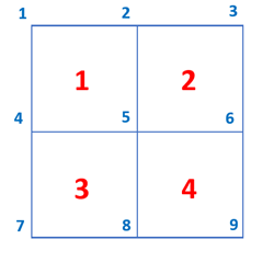
The main benefit of nodal-averaged results is a decreased results file size. Consider the simple 2x2 mesh shown in the below figure. Element-based results require 16 stored values (4-elements * 4-nodes-per-element) for each vector quantity, while the nodal-averaged results require only 9 stored values (1 per node) for each vector quantity—a 44% reduction. Savings will generally increase for 3D meshes, which involve more interior nodes.
Since nodal-averaged results are not stored by default, you must issue the OUTRES command to request them. The following output quantities are supported:
Item Label on
OUTRES | Quantity |
| NAR | All available nodal average results (includes all labels listed below) |
| NDST | Nodal-averaged stresses |
| NDEL | Nodal-averaged elastic strains |
| NDPL | Nodal-averaged plastic strains |
| NDCR | Nodal-averaged creep strains |
| NDTH | Nodal-averaged thermal and swelling strains |
Important: You should suppress the output of the related element quantities to avoid redundancy in the output values. For example, if you issue OUTRES,NDST to request storage of nodal-averaged stresses, you should also issue OUTRES,STRS,NONE to suppress storage of element-based nodal stresses.)
The following element types support nodal-averaged results:
Using Components to Request Nodal-Averaged Results for a Subset of Elements
In some cases, it may be advantageous to output nodal-averaged results for a subset of elements and element-based results for the remainder of the model. For example, this may be helpful if the model contains element types that do not support nodal-averaging. Another example is when element-based results are needed to evaluate mesh discretization error in certain areas of the model.
The Cname argument of OUTRES
enables you to specify a component (see the CM command)
containing elements for which the OUTRES specification is
active. Using components allows you to selectively activate nodal-averaged
results or element-based results for specific groups of elements.
For example, consider a model that contains BEAM188 elements, which do not support nodal-averaged results. The following commands select all BEAM188 elements in the model and output element-based stresses to the results file for that element type, while also outputting nodal-averaged results for all supported element types in the model.
ALLS,ALL
OUTRES,NDST,LAST    ! Request nodal-averaged stresses
OUTRES,STRS,NONE    ! Suppress element nodal stresses
ESEL,S,TYPE,,1      ! Select element type 1, which is BEAM188
CM,elgroup,ELEM     ! Create an element component containing BEAM188 elements
OUTRES,STRS,LAST,elgroup   ! Request element nodal stresses for the BEAM188 elements only
When postprocessing in POST1, you can view the output of the element solution for the beams using PRESOL,S and the output of the nodal-averaged result solution using PRNSOL,S.
Limitations for Nodal-Averaged Results
Nodal-averaged results are not valid for these analysis types:
Spectrum analysis
Cyclic symmetry analysis
You can print (PRNSOL) and plot (PLNSOL) nodal-averaged results in the POST1 general postprocessor (/POST1).
You can also print (PRVAR) and plot (PLVAR) nodal-averaged results in the POST26 time-history postprocessor (/POST26) after using the ANSOL command to store the results.
Nodal-averaged results are calculated during the solution phase (SOLVE) using the global Cartesian coordinate system and all selected elements and nodes. This cannot be changed. Therefore, operations on nodal-averaged results in POST1 or POST26 are done on a per-node basis rather than on a per-element basis. For that reason, any element-based operation performed in POST1 or POST26 has no effect on nodal-averaged results. For example, using ESEL or ESLN to select a subset of elements for output has no effect on nodal-averaged stresses and strains.
Using POST1 to View Nodal-Averaged Results
Nodal-averaged results are not stored in the database during or at the conclusion of the solution phase (SOLVE). They must be read into the database from the results file via the SET or SUBSET commands in POST1. Once in the database, the same operations can be used on nodal-averaged results as are available for the analogous element-based results. This includes saving (SAVE) and resuming (RESUME) the database, and postprocessing operations via the commands listed below.
| POST1 Commands that Support Nodal-Averaged Results | ||||
| APPEND | /GRAPHICS (FULL and POWER) | LCFILE | LCZERO | RESWRITE |
| AVPRIN | INRES | LCOPER | PLNSOL[a] | RSPLIT |
| DNSOL[a] | LCABS | LCSEL | PRNSOL[a] | SET |
| /EFACET | LCASE | LCSUM | RAPPND | *VGET [b] |
| *GET [b] | LCDEF | LCWRITE | RESCOMBINE | |
Using POST26 to View Nodal-Averaged Results
The time-history postprocessor does not read data from the database but instead uses the results file. After specifying the results file you want to postprocess (FILE command), use the POST26 commands listed below to define and view time-history variables for nodal-averaged results.
When DataKey = AUTO (the
default) is specified on the ANSOL command, either
element-based or nodal-averaged results may be used in the output of subsequent
commands. Starting at the first applicable time step, the availability of
element-based and nodal-averaged results is evaluated. If both are available,
then nodal-averaged results are used. If only one is available, then that data
type is used. If neither are available, then the data type to be used is not
determined and the checking repeats at the next time step. Once a data type is
determined, it is used for all subsequent time steps even if data of that type
is not available for a future time step. This process occurs independently for
every variable defined by ANSOL.
The following are examples of the
DataKey = AUTO logic.
Example 3.3: Case 1 - DataKey = AUTO Chooses Element-Based Data
| Load Step | 1 | 2 | 3 | 4 |
| Element-Based Data | X | X | X | |
| Nodal-Averaged Results | X | X |
Example 3.4: Case 2 - DataKey = AUTO Chooses Nodal-Averaged Results Data
| Load Step | 1 | 2 | 3 | 4 |
| Element-Based Data | X | X | X | |
| Nodal-Averaged Results | X | X |
Assumptions and Restrictions
In general, the nodal-averaged output is the same as the element-based output. However, there are some differences in data handling and other restrictions as listed below.
POST1 commands that manipulate solution results (APPEND, LCOPER, LCABS, RSPLIT) may give different numerical values when applied to nodal-averaged results compared to the same data stored as element results. This can happen because:
The operation is done on a per-node basis as opposed to a per-element basis.
The operation is applied to the nodal-averaged results after averaging, while it is applied to the element-based results before averaging.
The POST1 commands PRESOL and PLESOL are unaffected by the presence of nodal-averaged results. If element-based results are on the results file, these commands work the same as usual. If there are no element-based results on the results file, these commands show no results, regardless of whether nodal-average results are present on the results file.
The following command operations are not valid when viewing nodal-averaged results in POST1 or POST26 and cause nodal-averaged results to be blocked:
The following command operations are not valid when viewing nodal-averaged results in POST1 and cause nodal-averaged results to be blocked:
Issuing SUMTYPE,PRIN to combine principal stresses directly in a load case combination. Issuing this command blocks nodal-averaged stresses only. Nodal-averaged strains will still be available.
Issuing LCOPER with
Oper= LRPIN, SQUA, SQRT, or SRSS. These command operations erase the nodal-averaged results from the resulting load case.
Full Model Graphics vs. PowerGraphics — You can print or plot nodal-averaged results in both full model graphics and PowerGraphics modes. When PowerGraphics is enabled (/GRAPHICS,POWER), the results are averaged at a node using all member elements (not just the elements with faces on the surface) and with no separation for geometric or material discontinuities. Therefore, the PowerGraphics output is equivalent to the full model graphics output but only shows the appropriate surface nodes. This is equivalent to viewing the element solution in PowerGraphics after issuing the AVRES,1,FULL command. Performance improvements associated with PowerGraphics are maintained. Nodal-averaged results support the command /EFACET,2 for plotting midside nodes in PowerGraphics.
The nodal solution from an analysis consists of:
the degree-of-freedom solution, such as nodal displacements, temperatures, and pressures
the reaction solution calculated at constrained nodes - forces at displacement constraints, heat flows at temperature degree-of-freedom constraints, fluid flows at pressure degree-of-freedom constraints, and so on.
The degree-of-freedom solution is calculated for all active degrees of freedom in the model, which are determined by the union of all degree-of-freedom labels associated with all the active element types. It is output at all degrees of freedom that have a nonzero stiffness or conductivity and can be controlled by OUTPR,NSOL (for printed output) and OUTRES,NSOL (for results file output).
The reaction solution is calculated at all nodes that are constrained (D, DSYM, etc.). Its output can be controlled by OUTPR,RSOL and OUTRES,RSOL.
For vector degrees of freedom and corresponding reactions, the output during solution is in the nodal coordinate system. If a node was input with a rotated nodal coordinate system, the output nodal solution will also be in the rotated coordinate system. For a node with the rotation θxy = 90°, the printed UX solution will be in the nodal X direction, which in this case corresponds to the global Y direction. Rotational displacements (ROTX, ROTY, ROTZ) are output in radians, and phase angles from a harmonic analysis are output in degrees.