


After you have chosen a session in the Home page, Ansys Fluent's web interface opens your simulation session.
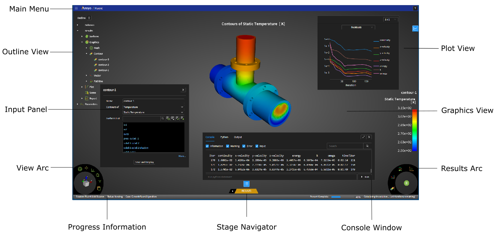
The graphical interface for Ansys Fluent's web interface is similar to the standard Fluent graphical interface, but different in some significant ways.
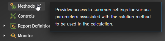
Note: When available, field-level user assistance provides guidance and information for a selected field.
The Main menu is where you can return to the Home page where you can sign into other remote sessions, as well as read in and write out your case and data files, and access key user preferences. See The Main Menu for more information.
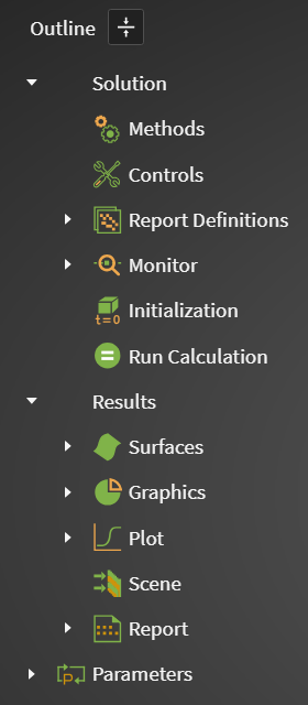
The Outline View is a simplified version of the Fluent's standard outline view. See The Outline View for more information.
The View Arc is a toolbar containing various view-related tools such as mesh display, fit-to-window, view orientation tools, and so on. See The View Arc for more information.
You can view pertinent details of your simulation status along the bottom of the window. See The Status Bar for more information.
The Stage Navigator is a tool that lets you navigate your simulation components (for example, Solution and Results). You can move through each component of the display to walk yourself though the stages of your simulation. Depending on the simulation mode, the outline view will change accordingly, presenting you with mode-specific tools and information. See The Stage Navigator for more information.
The Console is available to see more information about the solution progress, the solution transcript, and any messages that the solution may generate.
Note: Depending on the license level used in the Fluent session you are connected to (Enterprise or Premium), you can also enter and view Python commands in this window to augment your current simulation. This feature is not available if you are using the Pro level license.
See The Console Panel for more information.
The Results Arc is a toolbar with results-related tools such as contour, vector, pathline display tools. In addition, you can also perform solution-related tasks such as solution initialization and running calculations, and view your session's results-based objects (contours, vectors, etc.). See The Results Arc for more information.
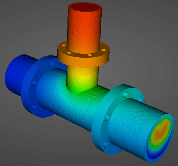
The Graphics View is where you can visualize your computational mesh, make graphics-related settings. See The Graphics Window for more information.
The Plots View is where you can visualize any 2D plotting formation such as residual plots, report definition plots, and any XY plots you may create. See The Plots View for more information.
Various input panels and dialog boxes are available for setting components of your simulation. See Property Panels for more information.
A Help menu is available (
 ) that presents an
overview of the user interface as well as a link to this document. In additon, an
About... option displays information related to the current
version of the web interface.
) that presents an
overview of the user interface as well as a link to this document. In additon, an
About... option displays information related to the current
version of the web interface.
- 47.3.1.1. The Main Menu
- 47.3.1.2. The Outline View
- 47.3.1.3. The Graphics Window
- 47.3.1.4. The View Arc
- 47.3.1.5. The Status Bar
- 47.3.1.6. The Stage Navigator
- 47.3.1.7. The Console Panel
- 47.3.1.8. The Results Arc
- 47.3.1.9. The Plots View
- 47.3.1.10. Property Panels
- 47.3.1.11. Working with Units
- 47.3.1.12. Working with Expressions
- 47.3.1.13. Editing Multiple Objects at Once
The main menu is equivalent to Fluent's standard File menu with many of the same options for reading, writing, importing, and exporting your simulation's various types of files (for example, mesh, case, data, etc.).
Read allows you to open common Fluent files such the mesh, case, case settings, data, case and data, field functions, injections, and profiles.
Note: When reading files, you can type in the file path and name in the corresponding field, or you can use the Browse... button to open a Select File(s) dialog box where you can browse the file system for the location and name of the file(s) you require. Note that the dialog box displays files on the "remote" file system (where Fluent is running) not the "local" machine (where the web browser is running).
Write allows you to save common Fluent files such as the case, data, and case and data files. You can also replace the mesh, as well as start and stop your transcript files.
Note: When writing files, you can type in the file path and name in the corresponding field, or you can use the Browse... button to open a Select File(s) dialog box where you can browse the file system for the location and name of the file(s) you require. Note that the dialog box displays files on the "remote" file system (where Fluent is running) not the "local" machine (where the web browser is running).
Import allows you to import various files into your session, including Chemkin and Functional Mock-up Unit (FMU) files.
Show Configuration displays the current session's configuration settings in the console window.
Preferences... displays the Fluent Preferences dialog box where user preferences are located when using the web interface.
The Theme option allows you to choose between the default dark color theme or a light color theme for the web interface.
The Show mesh on connection option allows you to choose whether or not to display the session's mesh in the graphics window immediately upon connecting to the session.
The Show all available settings (beta) option allows you to choose whether or not to make available more of the solver's more advanced settings and capabilities that have not been fully tested. This option is available when you run your Fluent session using the Enterprise license.
Note: Ansys Fluent's web interface only supports features that are available under Pro licensing (see Program Capabilities), such as access to a reduced set of Fluent solver capabilities allowing the solution of incompressible and compressible steady-state and transient, single-phase, turbulent, non-reacting flows, and heat transfer.
Additional features that are exposed using this preference have not been fully tested.
The Show Ansys logo option allows you to choose whether or not to display the Ansys logo in the graphics window.
Disconnect allows you to leave the current Fluent session from within the web interface.
Shutdown Fluent allows you to close the current Fluent session from within the web interface.
For more detailed information about these options, see File Ribbon Tab.
Ansys Fluent's web interface Outline View is similar to Fluent's standard outline view, allowing you to access and interact with various portions of your simulation project. Ansys Fluent's web interface displays the corresponding node according to the presence of the case or data file in Fluent. If data is present, then the Results branch is opened by default. so you can analyze your results. If only a case file is present, then the Solution branch is opened by default. If there is no case or data, then the Setup branch is available. Branches can be expanded and collapsed to suit your requirements. In addition, as you change stages using the Stage Navigator (The Stage Navigator), the Outline View changes accordingly.
Generally, you can add, delete, and rename objects by using the context menu on selected items in the tree. Depending on the context of where you are in the Outline View, certain objects have a context menu that has one or more of the following options available:
Rename
New
Copy to Clipboard (copying objects (such as report definitions, graphics objects such as contours, etc.) in the tree from within the same session or even between different sessions. Use this option to copy the selected object to your system clipboard, where you can then paste it into another selected object of the same type in the tree.
Paste from Clipboard (pasting objects (such as report definitions, graphics objects such as contours, etc.) in the tree from within the same session or even between different sessions. Use this option to paste copied objects from your system clipboard into another selected object of the same type in the tree.
Display (for showing selected objects in the graphics window)
Duplicate
Delete
Type (for reassigning type for cell zones or boundary conditions)
List Details
Note:
To select multiple items in the Outline View at the same time, hold down the Ctrl key while selecting non-adjacent items or hold down the Shift key while selecting adjacent items. Context menu options are available when applicable.
At the top level of the Outline View, cell zone and boundary condition can be displayed in various ways through the Group By context menu option where you have the choice of displaying a List View, by Name, by Adjacency (for boundaries only), or by Zone Type (the default).
The Outline View can be relocated by hovering the mouse over the top of the tree until the cursor changes from the 'pointer' to the 'pan' symbol.
The graphics window displays the graphical output of your simulation (mesh, contours, pathlines, etc.). Along with being able to select one or more objects, rotate, zoom, pan, etc. within the window, you can also interact with the contents by right-clicking to display a context menu that corresponds with your current stage.
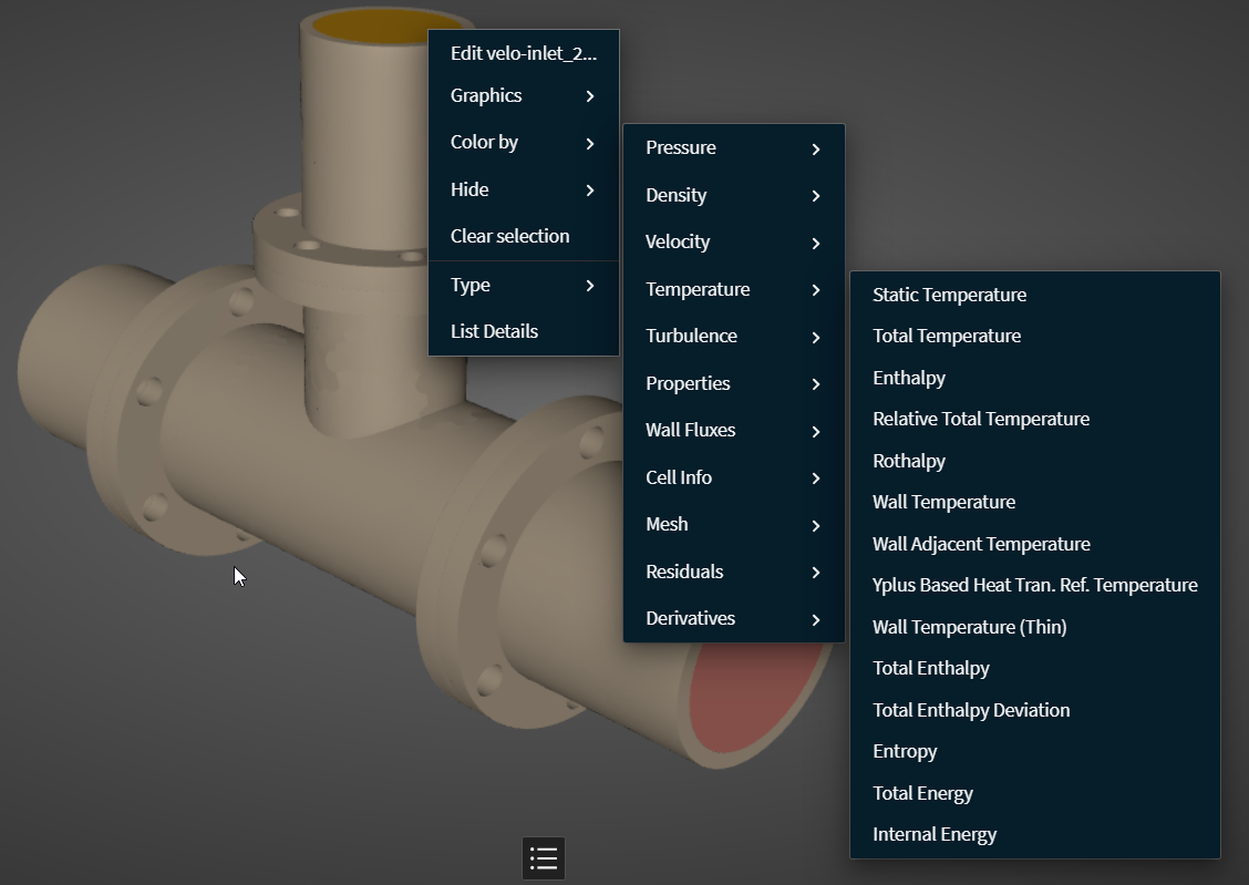
Supported operations within the graphics window depend on the selected object(s) and include:
Single selection
Box selection
Interactively edit/show/hide selected items (via context menu, e.g., changing the zone type, etc.)
Interactively create additional graphics objects (via context menu)
Interactively move and resize the color map for results-based plots such as contours, vectors, etc. You can restore the color map to its original location by using the Shift+r key combination.
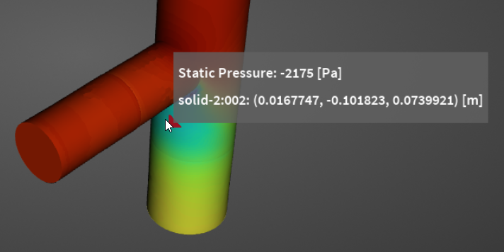
Interactively use the mouse to probe your results to visualize specific values in specific areas. This is available using the corresponding mode in the View Arc (see The View Arc) where you click a portion of the graphics object (for example, contour, vector, etc.) to display a listing of results-based details for the specified portion of the plot, such as its position, the name of the surface, and the current value of the field variable at that location. You can add multiple probes to the display by holding down the Ctrl key as you pick probe locations that persist as you manipulate the plots in the graphics window. Press ESC to dismiss the probe display(s). Probe information is preserved when you save the graphics view to a file.
For more general information about graphics windows in Fluent, see Displaying Graphics.
Ansys Fluent's web interface includes a View Arc, a circular toolbar located within the window, containing various view-related tools such as mesh display, fit-to-window, view orientation tools, and so on.
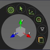
Options include:
Mesh display options: tools that allow you to create a new mesh object or display an existing mesh object.
Left mouse button options: tools that allow you to choose between various left mouse behaviors such as selection, rotation, panning, zooming in or out, probing, etc. Note that the mouse icon changes according to your selection.
Note that by default, the rotation mode allows rotation about the center of the screen. You can rotate around a specific point using the Ctrl key while in rotation mode.
View options: tools that allow you to quickly orient the display to your liking (for example, isometric view, +/-X, +/-Y, and +/-Z directions).
Fit to window: tool that allows you to quickly fit the display to the window.
Filter Selections: tool that allows you to quickly filter your selections in the graphics window based on some or all of the available types.
Save to clipboard or file: tools that allow you to quickly save the display to the clipboard or to a file.
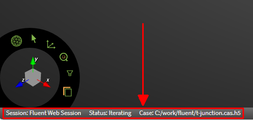
General information about your simulation can be found in the status bar at the bottom of the window.
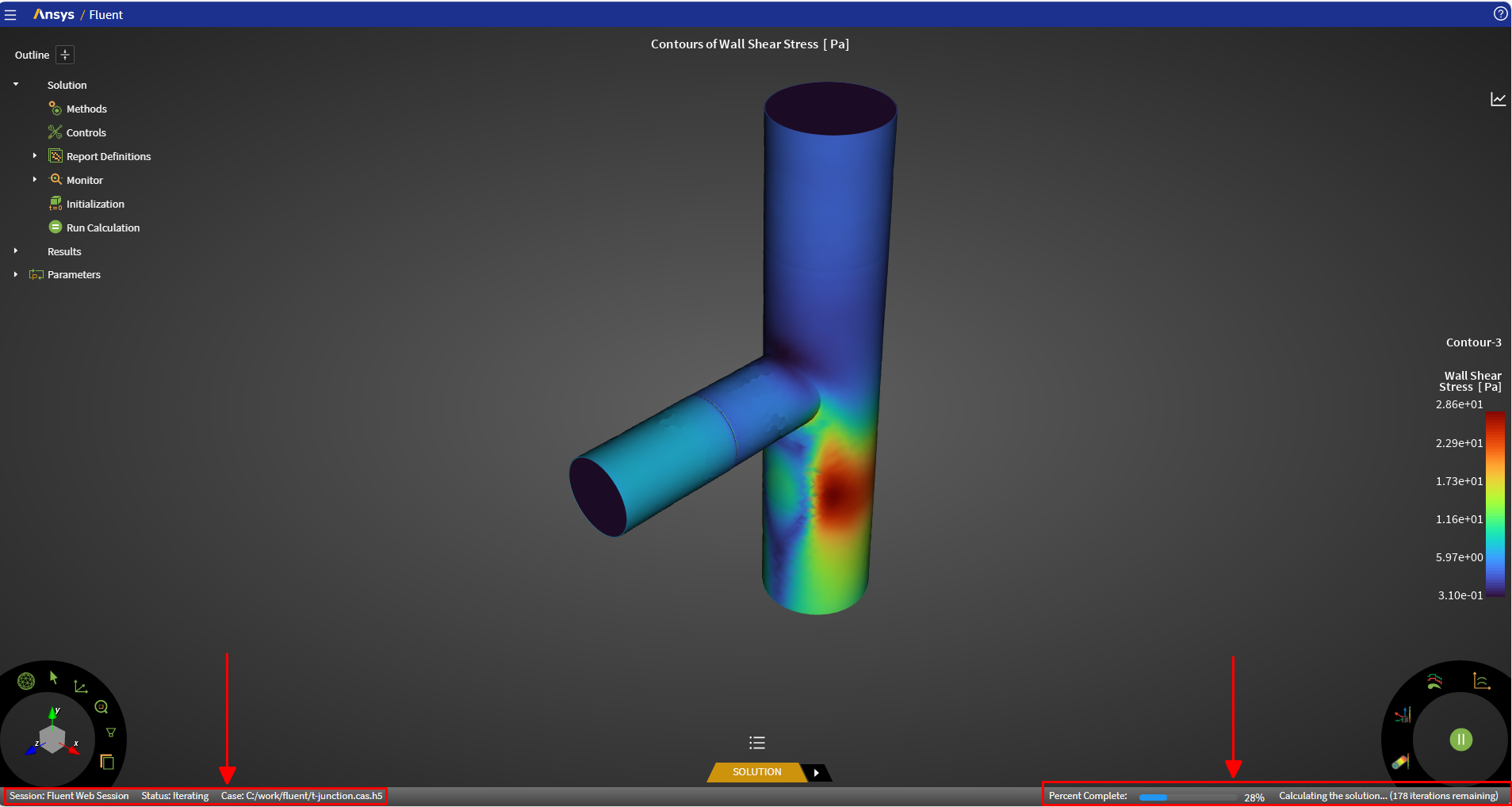
Details about your simulation (session name, status, case name) can be found in the left side of the status bar.
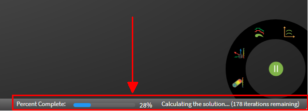
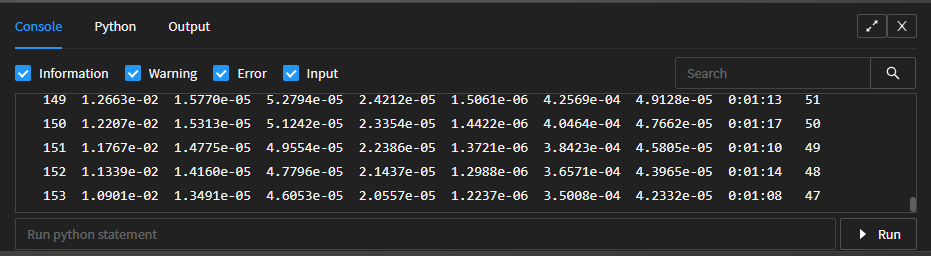
While a calculation is underway, you can view its progress in the status bar at the bottom of the browser window.
The Stage Navigator is a means of traversing (using the arrows) through the various stages of your simulation. As you do, the Outline View (The Outline View) changes to expose the relevant nodes that correlate to the various stages in the simulation.

The Console panel is your primary access to any informative messages, Python commands,
and output from a simulation. To open the Console panel, click the corresponding icon
(![]() ).
).
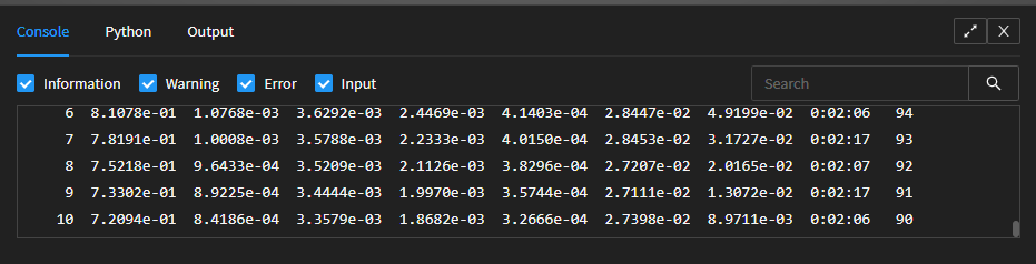
Console Messaging
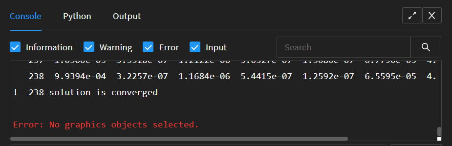
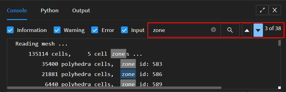
The panel has a Console tab that will contain transcript data, informative messages about relevant simulation progress, warnings, errors, etc.
You are alerted of any errors via changes to the Console icon, for example:
You can also filter messages by types – information, warning, error, and output.
You can also search the Console output using the Search field.
Access to Python
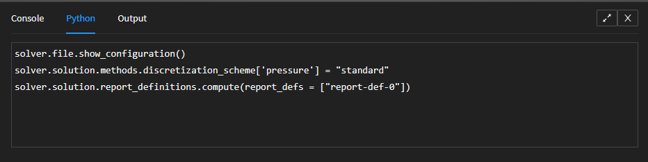
The Python tab shows Python commands while you interact with the session.
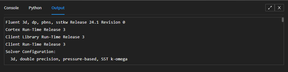
Viewing Simulation Output
The Output tab contains basic output messages from the solver.
Note: The window can be relocated by hovering the mouse over the top of the tree until the cursor changes from the 'pointer' to the 'pan' symbol. You can also make the window full size or close it altogether using the icons in the upper right corner. You can also close the window by clicking the corresponding icon above the Stage Navigator.
Note: You can capture all text within the window by using Ctrl-A.
Depending on the license level used in the Fluent session you are connected to (Enterprise or Premium), you can view and enter Python commands in this window to augment your current simulation.
Note: This feature is not available if you are using a Pro level license.
In addition, the Console window also has a Python tab that allows you to view and enter Python commands and directly interact with the Fluent session using the collection of Pythonic interfaces for Fluent.
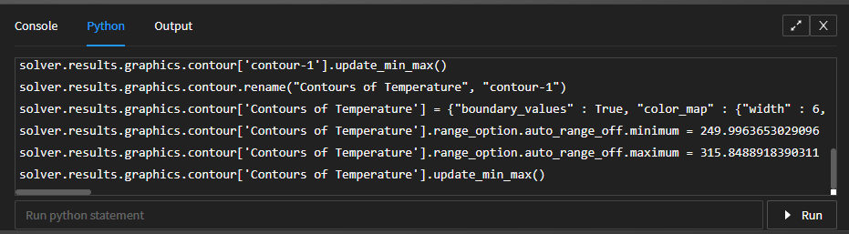
The Console window, the Python window, and the Output window all have a command entry field where you can type a Python command. Once you type in your command, click the Run button to run the command, or click the Clear button to remove the command from the field.
Note: For both the Console window and the Python window, you can capture all text within the window by using Ctrl-A.
Ansys Fluent's web interface includes a Results Arc, a circular toolbar located within the window, containing various results-related tools such as displaying contours, vectors, and so on.

Options include:
Contour display options: tools that allow you to create a new contour object or display an existing contour object.
Vector display options: tools that allow you to create a new vector object or display an existing vector object.
Pathline display options: tools that allow you to create a new pathline object or display an existing pathline object.
XY plot display options: tools that allow you to create a new XY plot object or display an existing XY plot object.
Mirror plane options: tools that allow you to create a new mirror plane or show/hide an existing mirror plane(s). See Creating and Displaying Mirror Plane Objects for details.
You can also use the Calculate button to quickly initialize or to start a calculation.
Once the calculations are in progress, you can choose to either Interrupt or Pause the solution progression.
Once the calculations are paused, you can choose to either Interrupt or Resume the solution progression.
Note: There is a subtle difference between pausing and interrupting your calculations, depending on whether you are running a transient or a steady-state simulation, or if you are running a journal file or not.
When you choose to Pause a solution, for steady-state simulations, the solver progresses until it reaches the earliest safe stopping point after the current iteration, whereas for transient simulations, the solver progresses until it reaches the earliest safe stopping point after the current time step.
When you choose to Interrupt a solution and you are running a journal file, the act of interrupting the solution leads the solver to stop and exit from the journal file.
Note: While running standard Fluent in batch mode, by default, Fluent does not exit
when the iterations are complete, unless an explicit end-of-file mechanism (that is,
when standard input (stdin) is not present) is manually in
place via a script, etc.
During a batch calculation, if an error occurs, or if you choose to interrupt the batch calculation, then the journal is stopped. If the web server is running, Fluent will remain active and available, allowing you to interact with it using the web interface just as you would in an interactive session.
If there is a specified value for the Idle Timeout preference in Fluent, then Fluent will shut down if there is no activity in the web interface after the specified idle time out period. Just as in Fluent, a countdown message is displayed in the web interface before shutting down the session due to inactivity. For instance:
This process has been idle for 33 secs, It will start exiting
after 27 secs. The case and data will be saved before
exiting. Press Close to continue to work.
If there is no specified value for the Idle Timeout preference in Fluent, one of two things can happen, regardless of if there is an explicit
exitcommand in the journal file:If an explicit end-of-file mechanism is in place for the connected batch session, then a timeout period of 30 minutes is automatically applied and a corresponding message will immediately appear in the console:
Setting Idle time of 30 min after which session will exit.
This timeout period is only started when the journal is stopped and when the batch session is transformed into an interactive session.
If an explicit end-of-file mechanism is not in place for the connected batch session, then no message appears, meaning that Fluent is still running and will need to be manually stopped.
Note: While calculations are progressing, you are intentionally not allowed to make changes to your simulation settings and/or perform certain actions, such as:
Reading case/data files.
Starting another calculation.
Editing model settings.
Editing solution and/or initialization settings, such as the number of iterations, timesteps, etc.
Ansys Fluent's web interface includes a Plots View, where you can visualize your calculation's residual plots, as well as any report definition plots for your simulation. Click the title to open the corresponding plot.
Note: The window can be relocated by hovering the mouse over the top of the window until the cursor changes from the 'pointer' to the 'pan' symbol. You can minimize the window using the icons in the upper right corner.
When the window is not in its docked position, you can also resize the window by hovering the mouse over the bottom edge or the left edge of the window until the cursor changes to the 'edge' symbol.
Hovering the mouse over the plots reveals specific data values and exposes some assorted controls for plotting:
Download plot as png: saves the plot as a PNG file, prompting you to browse and specify the name and location of the file.
Zoom: use the mouse to draw a box that the view will zoom into.
Pan: use the mouse to pan across the XY plot.
Zoom in: zoom into the current view.
Zoom out: zoom out of the current view.
Auto-scale: resets the view to the original size and scale.
Reset Axes: resets the X and Y axes.
For more information about using plots, see Working With Plots and Your Simulation Results.
You can access and edit the attributes of various objects in your simulation through the various property panels that are available. The properties panels are similar to Fluent's task pages and dialog boxes, in that they allow you to define settings, enter, and postprocess results. Note that your settings are saved as you define them in a properties panel. There are also some dialog boxes (which you may open from the Outline View or settings in the properties panel) which may have an explicit mechanism to save your work.
The content of the various property panels is similar to those found in Fluent, however, there are some differences. For instance, the visual layout of the groups, labels, and controls is more streamlined, as are the handling of units and expressions.
Unit management is more flexible from Fluent's handling of units. Using the corresponding drop-down menu, you can change the units accordingly on a case-by-case basis, if desired.
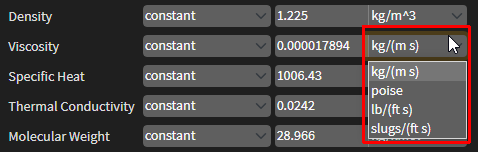
Units can be managed from the General properties in the Outline View.
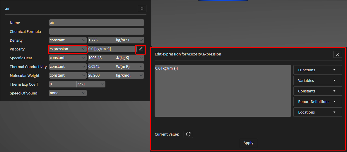
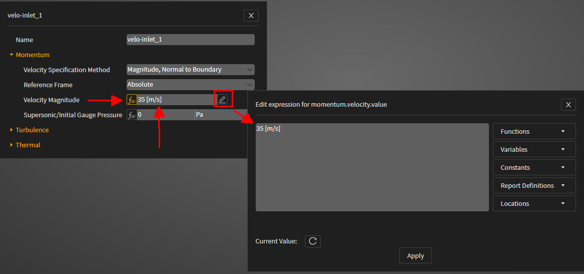
Handling expressions is similar to Fluent, however, there are two ways to work with expressions in Ansys Fluent's web interface.
Choosing an expression for certain material properties, when available. In these cases, you can choose to represent your material property using an expression by choosing expression from the corresponding drop-down menu. The expression is listed, and you can then edit the expression using the corresponding icon (
 ) to
open the expression editor.
) to
open the expression editor.Using an expression for boundary conditions, when available. In these cases, an expression icon (
 ) can be selected
(
) can be selected
( ) to enable
the use of an expression for a property. When selected, the expression is presented
and can be changed by clicking the corresponding icon ( ) to open the expression
editor.
) to enable
the use of an expression for a property. When selected, the expression is presented
and can be changed by clicking the corresponding icon ( ) to open the expression
editor.
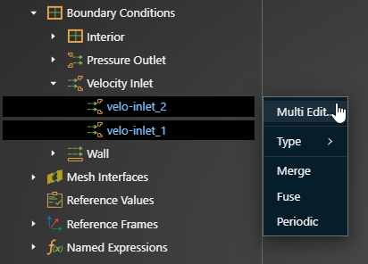
Especially for boundary conditions of the same type, you are able to edit more than one object at a time and apply one or more of an object's properties to another. For instance, you can select two velocity-inlet conditions, right-click and select Multi-Edit from the context menu.
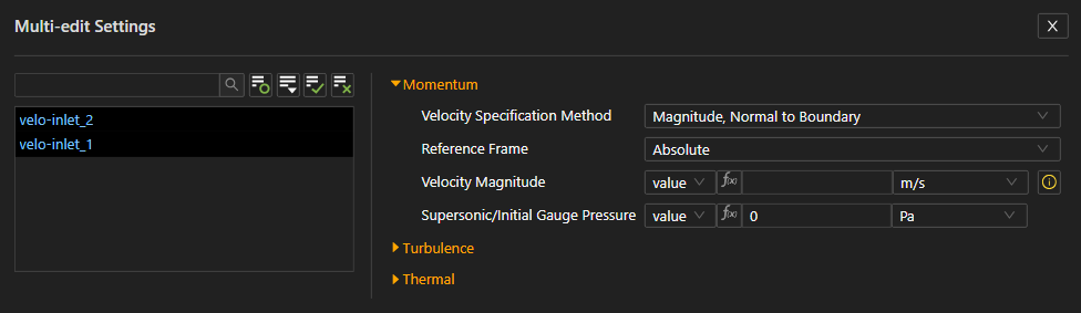
This displays the Multi-Edit Settings panel where you can see the selected objects, and their common properties.
For common, active properties, an informational icon (![]() ) next to an empty property
indicates a property where you can choose a value from one of the selected objects.
) next to an empty property
indicates a property where you can choose a value from one of the selected objects.
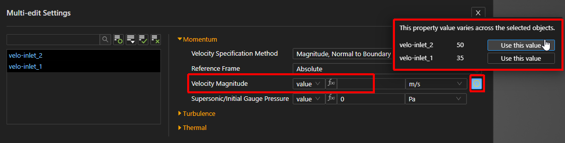
For more information about multiple selection using Fluent, see Editing Multiple Boundary Conditions at Once.
One aspect of Ansys Fluent's web interface is the ability to interact with and change your Fluent simulation set up within the web interface. The Setup branch of the Outline view allows you to access and modify simulation settings (models, materials, cell zone and boundary conditions, etc.).
Note: While calculations are progressing, you are intentionally not allowed to make changes to your simulation settings and/or perform certain actions, such as:
Reading case/data files.
Starting another calculation.
Editing model settings.
Editing solution and/or initialization settings, such as the number of iterations, timesteps, etc.
The following sections describe operations available for setting up your simulation in Ansys Fluent's web interface.
- 47.3.2.1. Accessing General Settings
- 47.3.2.2. Accessing Model Settings
- 47.3.2.3. Accessing Material Settings
- 47.3.2.4. Accessing Cell Zone Settings
- 47.3.2.5. Accessing Boundary Condition Settings
- 47.3.2.6. Accessing Reference Values Settings
- 47.3.2.7. Accessing Reference Frame Settings
- 47.3.2.8. Accessing Named Expression Settings
You are able to access your simulation's general properties using Ansys Fluent's web interface.
![]() Setup → General
Setup → General
From here, you can view or make changes to settings such as the solver type or operating conditions such as the gravitational acceleration, and unit settings. The available general settings are similar to those found in the standard Fluent solver. For more detailed information about them, see General Task Page.
You are able to access your simulation's model properties using Ansys Fluent's web interface.
![]() Setup → Models
Setup → Models
From here, you can view or make changes to the models available to your session such as the consideration of energy, turbulence (viscous), species, and discrete phase. The available model settings are similar to those found in the standard Fluent solver. For more detailed information about them, see the Fluent documentation (e.g., Models Task Page).
Energy: Energy Dialog Box
Viscous: Viscous Model Dialog Box
Species: Species Model Dialog Box
Discrete Phase: Discrete Phase Model Dialog Box
You are able to access your simulation's material properties using Ansys Fluent's web interface.
![]() Setup → Materials
Setup → Materials
From here, you can create new or view and make changes to the fluid and solid (and mixture, if applicable) materials available in your session, such as the material's density, specific heat, thermal conductivity, molecular weight, and so on. You can even access other material databases as well. The available material settings are similar to those found in the standard Fluent solver. For more detailed information about creating new and editing existing materials, see Create/Edit Materials Dialog Box.
You are able to access your simulation's cell zone conditions using Ansys Fluent's web interface.
![]() Setup → Cell Zone
Conditions
Setup → Cell Zone
Conditions
From here, you can create new or view and make changes to the fluid and solid cell zones conditions that are available in your session, such as a cell zone's assignment, reference frame, porosity, motion, source terms, and so on. The available settings are similar to those found in the standard Fluent solver. For additional information about cell zone properties in the standard Fluent solver, see Cell Zone Conditions Task Page.
For more information about Fluid cell zone conditions, see Fluid Dialog Box.
For more information about Solid cell zone conditions, see Solid Dialog Box.
Note: Cell zones can be displayed in the Outline View in various ways through the Group By context menu option where you have the choice of displaying a List View, by Name, or by Zone Type (the default).
You are able to access your simulation's boundary conditions using Ansys Fluent's web interface.
![]() Setup → Boundary
Conditions
Setup → Boundary
Conditions
From here, you can create new or view and make changes to existing boundary conditions that are available in your session, such as a inlets, outlet, walls, and so on. The available settings for each boundary type are similar to those found in the standard Fluent solver. For more detailed information about them, see Boundary Conditions Task Page.
Note: Boundary condition can be displayed in the Outline View in various ways through the Group By context menu option where you have the choice of displaying a List View, by Name, by Adjacency, or by Zone Type (the default).
You are able to access your simulation's reference values using Ansys Fluent's web interface.
![]() Setup → Reference Values
Setup → Reference Values
From here, you can create new reference values or view and make changes to existing reference values that are available in your session, such as area, density, enthalpy, length, pressure, and so on. The available settings are similar to those found in the standard Fluent solver. For more detailed information about them, see Reference Values Task Page.
You are able to access your simulation's reference frames using Ansys Fluent's web interface.
![]() Setup → Reference Frames
Setup → Reference Frames
From here, you can create new reference frames or view and make changes to existing reference frames that are available in your session, such as its motion or the initial state. The available settings are similar to those found in the standard Fluent solver. For more detailed information about them, see Reference Frame Dialog Box.
You are able to access your simulation's named expressions using Ansys Fluent's web interface.
![]() Setup → Named Expressions
Setup → Named Expressions
From here, you can create new named expressions, create and view plots of your expressions, or view and make changes to existing named expressions that are available in your session. The available settings are similar to those found in the standard Fluent solver. For more detailed information about them, see Expression Manager Dialog Box.
Another aspect of Ansys Fluent's web interface is the ability to interact with and change your Fluent simulation settings within the web interface.
Note: While calculations are progressing, you are intentionally not allowed to make changes to your simulation settings and/or perform certain actions, such as:
Reading case/data files.
Starting another calculation.
Editing model settings.
Editing solution and/or initialization settings, such as the number of iterations, timesteps, etc.
The following sections describe operations available for solution settings in Ansys Fluent's web interface.
Various means of setting your solution methods are available
![]() Solution → Methods
Solution → Methods
From here, you can view and make changes to solution methods, such as the discretization scheme for pressure, momentum, and so on. The available settings are similar to those found in the standard Fluent solver. For more detailed information about them, see Solution Methods Task Page.
Various means of setting your solution controls are available
![]() Solution → Methods
Solution → Methods
From here, you can view and make changes to solution controls, such as relaxation factors, equations, limits, and so on. The available settings are similar to those found in the standard Fluent solver. For more detailed information about them, see Solution Controls Task Page.
Various means of setting your solution's report definitions are available
![]() Solution → Report
Definitions
Solution → Report
Definitions
From here, you can create new or view and make changes to existing report definitions in your session, such as report definitions for mesh, surface, volume, force, lift, drag, moment, flux, user-defined, and single-valued expressions.
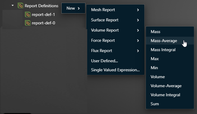
The available settings are similar to those found in the standard Fluent solver. For more detailed information about them, see Report Definitions Dialog Box.
Various means of setting your solution's monitors are available
![]() Solution → Monitors
Solution → Monitors
From here, you can create new or view and make changes to existing solution monitors in your session, such as residual, report file, report plot, and convergence condition monitors. The available settings are similar to those found in the standard Fluent solver. For more detailed information about them, see the Fluent documentation.
Residuals (see Residual Monitors Dialog Box)
Report Files (see Report File Definitions Dialog Box)
Report Plots (see Report Plot Definitions Dialog Box)
Convergence Conditions (see Convergence Conditions Dialog Box)
Various means of initializing your solution are available
![]() Solution → Initialization
Solution → Initialization
From here, you can view and make changes to solution controls such as the initialization type, the reference frame, various default solution settings, and so on. The available settings are similar to those found in the standard Fluent solver. For more detailed information about them, see Solution Initialization Task Page.
Note: You can also initialize and start the calculations using the Results Arc
(![]() ).
).
Various means of running the calculations methods are available
![]() Solution → Run Calculation
Solution → Run Calculation
From here, you can view and make changes to solution controls important when running the calculations, such as time step settings, the number of iterations, reporting interval, and so on. The available settings are similar to those found in the standard Fluent solver. For more detailed information about them, see Run Calculation Task Page.
Note: You can also initialize and start the calculations using the Results Arc
(![]() ).
).
Once a calculation is started, you can either interrupt or pause the Fluent solver. When you interrupt a calculation, Fluent formally exits the iteration loop, however, when you pause a calculation, the Fluent solver is paused without exiting the iteration loop.
When using a journal file, interrupting a calculation will completely exit the journal file while pausing a calculation lets you continue to use your journal file.
Note: To improve performance, you should pause Fluent when you are post-processing results during a calculation.
A key aspect of Ansys Fluent's web interface is the ability to analyze the results of your calculations as the Fluent client is solving a fluid flow simulation. In addition, using Ansys Fluent's web interface, you can create and edit your results as the solver is running.
The following sections describe operations available for graphics objects in Ansys Fluent's web interface.
- 47.3.4.1. Working With Surfaces and Your Simulation Results
- 47.3.4.2. Working With Graphics Objects and Your Simulation Results
- 47.3.4.3. Working With Plots and Your Simulation Results
- 47.3.4.4. Creating and Displaying Scenes and Your Simulation Results
- 47.3.4.5. Creating and Displaying Reports for Your Simulation Results
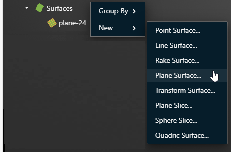
You can create different types of surfaces to visualize your results, including points, lines, rakes, planes, iso-surfaces, iso-clips, transform surfaces, plane slices, sphere slices, and quadric surfaces. Values are interpolated to the smoothed out boundary lines.
For more information on working with surfaces in Fluent, see Creating Surfaces and Cell Registers for Displaying and Reporting Data.
- 47.3.4.1.1. Creating and Displaying Point Surfaces
- 47.3.4.1.2. Creating and Displaying Line Surfaces
- 47.3.4.1.3. Creating and Displaying Rake Surfaces
- 47.3.4.1.4. Creating and Displaying Plane Surfaces
- 47.3.4.1.5. Creating and Displaying Iso Surfaces
- 47.3.4.1.6. Creating and Displaying Iso-Clip Surfaces
- 47.3.4.1.7. Creating and Displaying Transform Surfaces
- 47.3.4.1.8. Creating and Displaying Plane Slice Surfaces
- 47.3.4.1.9. Creating and Displaying Sphere Slice Surfaces
- 47.3.4.1.10. Creating and Displaying Quadric Surfaces
You may be interested in displaying results at a single point in the domain. For example, you may want to monitor the value of some variable or function at a particular location. To do this, you must first create a "point" surface, which consists of a single point. When you display node-value data on a point surface, the value displayed is a linear average of the neighboring node values. If you display cell-value data, the value at the cell in which the point lies is displayed.
![]() Results
→ Surfaces → Point
Results
→ Surfaces → Point
![]() New
New
Specify the location of the point. Enter the coordinates (x, y, z) under Coordinates.
A line is simply a line that extends up to and includes the specified endpoints; data points will be located where the line intersects the faces of the cell, and consequently may not be equally spaced.
![]() Results
→ Surfaces → Line
Results
→ Surfaces → Line
![]() New
New
Specify the location of the P0 (start point).
Specify the location of the P1 (end point).
A rake consists of a specified number of points equally spaced between two specified endpoints.
![]() Results
→ Surfaces → Rake
Results
→ Surfaces → Rake
![]() New
New
Specify the location of the P0 (start point).
Specify the location of the P1 (end point).
Set the Number of points to include in the rake surface.
To display flow-field data on a specific plane in the domain, you will use a plane surface. You can create surfaces that cut through the solution domain along arbitrary planes (3D cases only).
There are three types of plane surfaces that you can create:
Coordinate system-based—the plane is created in the YX, ZX, or XY directions, bounded by the extents of the domain.
Point and normal—the plane orientation is determined by selecting a point and specifying a direction normal to that plane. The extents of the plane are the edges of the domain.
Three points—the plane orientation and extents are bounded by three points that you can specify.
You can create a plane surface by specifying the Method as yz, xz, xy then specify the corresponding X, Y, or Z value.
If you want to If you want to display results on cells that have a constant value for a specified variable, you will need to create an iso-surface of that variable. Generating an iso-surface based on x, y, or z coordinate, for example, will give you an x, y, or z cross-section of your domain; generating an iso-surface based on pressure will enable you to display data for another variable on a surface of constant pressure. You can create an iso-surface from an existing surface or from the entire domain. Furthermore, you can restrict any iso-surface to a specified cell zone.
![]() Results
→ Surfaces → Iso-Surface
Results
→ Surfaces → Iso-Surface
![]() New
New
To create an iso-surface:
Click the Field drop-down menu to specify the field you want to view.
(Optional) Specify a Surface to only display iso-values on specific surfaces.
(Optional) Specify a Zone to only display iso-values on specific zones.
Set the range by specifying the Minimum and Maximum.
Enter the iso-values into the Iso-Value field. You can enter multiple iso-values into the field separated by spaces.
If you have created a surface, but you do not want to use the whole surface to display data, you can clip the surface between two isovalues to create a new surface that spans a specified subrange of a specified scalar quantity. The clipped surface consists of those points on the selected surface where the scalar field values are within the specified range.
![]() Results
→ Surfaces → Iso Clip
Results
→ Surfaces → Iso Clip
![]() New
New
Specify the variables for Clip to Values of as well as one or more Clip Surfaces and click Display.
You can create a new data surface from an existing surface by rotating and/or translating the original surface. For example, you can rotate the surface of a complicated turbomachinery blade to plot data in the region between blades. You can also create a new surface at a constant normal distance from the original surface.
![]() Results
→ Surfaces → Transform
Surface
Results
→ Surfaces → Transform
Surface ![]() New
New
Specify one or more Surfaces, as well as any rotational and/or translational properties as needed, then click Display.
If you want to display data on a planar surface, you can specify the surface by entering the coefficients of the function that defines it.
![]() Results
→ Surfaces → Plane Slice
Results
→ Surfaces → Plane Slice
![]() New
New
The surface will consist of all points on the domain that satisfy the equation
 . You will specify ix (the coefficient of
 ), iy (the coefficient of
  ), iz (the coefficient of
  ), and Distance (the distance of the line or plane
from the origin), then click Display.
), and Distance (the distance of the line or plane
from the origin), then click Display.
If you want to display data on a spherical surface, you can specify the surface by entering the coefficients of the function that defines it.
![]() Results
→ Surfaces → Sphere Slice
Results
→ Surfaces → Sphere Slice
![]() New
New
The surface will consist of all points on the domain that satisfy the equation
 . You will specify x0, y0,
z0 (the
. You will specify x0, y0,
z0 (the  ,
,  , and
, and  coordinates of the sphere or circle’s center) and
r (the radius)
coordinates of the sphere or circle’s center) and
r (the radius)
Specify one or more Center properties as needed, as well as a Radius, then click Display.
If you want to display data on a general quadric surface, you can specify the surface by entering the coefficients of the quadric function that defines it. This feature provides you with an explicit method for defining surfaces.
![]() Results
→ Surfaces → Quadric Surface
Results
→ Surfaces → Quadric Surface
![]() New
New
The surface will consist of all points in the domain that satisfy the general
quadric function  . You will specify the coefficients of the quadric function
 (the coefficients of the terms
  ,
,  ,
,  , xy, yz, zx, x, y, z and the constant term).
Specify one or more Attributes as needed, as well as a Value, then click Display.
Ansys Fluent's web interface can create new, and access, display, and edit existing graphics objects that are defined on the client.
Note: By default, Ansys Fluent's web interface displays graphics object results using the field-velocity color map.
Note: The name of the graphics object is used as the title of the display.
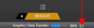
Note: You can cancel the rendering of complex graphical objects
that may take an excessive amount of time by clicking the Stop
icon (![]() ) near the
progress bar while the rendering is taking place.
) near the
progress bar while the rendering is taking place.
The following sections describe operations available for graphics objects in Ansys Fluent's web interface.
You can draw the mesh for all or part of your domain.
![]() Results
→ Graphics → Mesh
Results
→ Graphics → Mesh
![]() New
New
For the new mesh object, make the necessary changes and Click Display to see the new mesh object in the graphics view.
For more information on working with meshes in Fluent, see Displaying the Mesh.
Ansys Fluent's web interface enables you to plot contour lines or profiles. Contour lines are lines of constant magnitude for a selected variable (isotherms, isobars, and so on).
![]() Results
→ Graphics → Contour
Results
→ Graphics → Contour
![]() New
New
For a new contour object, make the necessary changes and click Display to see the new contour object in the graphics view.
For more information on working with contours in Fluent, see Displaying Contours and Profiles.
You can draw vectors in the entire domain, or on selected surfaces. By default, one vector is drawn at the center of each cell (or at the center of each facet of a data surface), with the length and color of the arrows representing the velocity magnitude. The spacing, size, and coloring of the arrows can be modified, along with several other vector plot settings. Velocity vectors are the default, but you can also plot vector quantities other than velocity. Note that cell-center values are always used for vector plots, and you cannot plot node-averaged values.
![]() Results
→ Graphics → Vector
Results
→ Graphics → Vector
![]() New
New
For the new vector object, make the necessary changes and click Display to see the new vector object in the graphics view.
For more information on working with vectors in Fluent, see Displaying Vectors.
Pathlines are used to visualize the flow of massless particles in the problem domain. The particles are released from one or more surfaces present in your domain.
![]() Results
→ Graphics → Pathline
Results
→ Graphics → Pathline
![]() New
New
For the new pathline object, make the necessary changes and click Display to see the new pathline object in the graphics view.
For more information on working with pathlines in Fluent, see Displaying Pathlines.
You can create special view-related objects for mirroring your geometry about a symmetrical plane using the Results Arc.
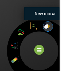
You can also create new mirror planes through the Outline View.
![]() Results
→ Graphics → Views → Mirror
Planes
Results
→ Graphics → Views → Mirror
Planes![]() New
New
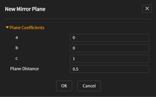
In either case, this displays the New Mirror Plane dialog box (see Creating New Mirror Planes).
Once created, you can access your mirror planes through the arc (a check mark next to the name of the mirror plane indicates that it is visible):
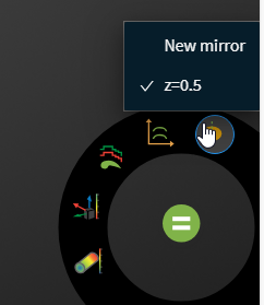
You can also access existing mirror planes through the Outline View:
![]() Results
→ Graphics → Views → Mirror
Planes
Results
→ Graphics → Views → Mirror
Planes

For more information on working with mirror planes in Fluent, see Mirroring and Periodic Repeats.
Using the New Mirror Plane dialog box, you can specify the Plane Coefficients and the Plane Distance.
When you have multiple mirror planes available, but only need to use a select few, you can open the Apply Mirror Planes dialog box to pick and choose which planes to use.
![]() Results
→ Graphics → Views
Results
→ Graphics → Views
![]() Apply Mirror Planes
Apply Mirror Planes
This displays the Apply Mirror Planes dialog box:
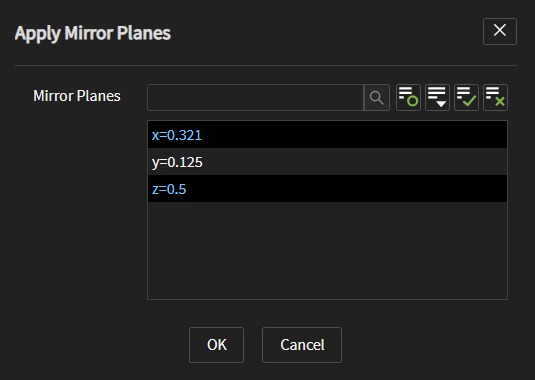
Use the Apply Mirror Planes dialog box to pick which mirror planes to employ.
In addition to the many graphics tools already discussed, Ansys Fluent's web interface also provides tools that enable you to generate XY plots of solution, file, profile, and residual data.
Note: Plots can be relocated by hovering the mouse over the top of the plot window until the cursor changes from the 'pointer' to the 'pan' symbol.
When the window is not in its docked position, you can also resize the window by hovering the mouse over the bottom edge or the left edge of the window until the cursor changes to the 'edge' symbol.
An XY (abscissa/ordinate) plot is a line and/or symbol chart of data. Virtually any defined variable or function is accessible for this type of plot.
![]() Results
→ Plot → XY Plot
Results
→ Plot → XY Plot
![]() New
New
For the new XY plot object, make the necessary changes and click Display to see the new XY plot object in a separate window.
You can drill down into the specifics of the plot data interactively. See Analyzing Data in Plots for details.
For more information on working with XY plots in Fluent, see XY Plots.
A histogram plot is a bar chart of data. It is a representation of a frequency of distribution by means of rectangles of widths representing class intervals and with areas proportional to the corresponding frequencies. The web interface allows you to generate histogram data.
![]() Results
→ Plot → Histogram
Results
→ Plot → Histogram
To generate histogram data, make the necessary changes (to such properties as Auto Range, Number of Divisions, and whether or not to include All Zones). Click Print to see the new histogram plot details in a console panel, or click Plot to see a graphical representation of the data.
For more information, see Histograms.
A cumulative plot allows you to analyze the development of force, moments, or coefficients for your model in the any desired location or direction.
![]() Results
→ Plot → Cumulative
Results
→ Plot → Cumulative
To generate cumulative data, make the necessary changes (such as setting the cumulative force/moment or their coefficients under Option, one or more Zones, Split Direction, Number of Divisions, and the Force Direction) and click Plot to see the new cumulative plot details.
For more information, see Cumulative Force, Moment, and Coefficients Plots.
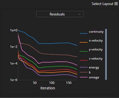
Residual history is displayed using an XY plot. The abscissa of the plot corresponds to the number of iterations and the ordinate corresponds to the log-scaled residual values.
You can drill down into the specifics of the plot data interactively. See Analyzing Data in Plots for details.
For simulations that have report definitions, you can see the corresponding plot in the Plot View.
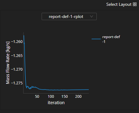
Note: Click the title of the plot to display other report definition plots that are also be available
You can drill down into the specifics of the plot data interactively. See Analyzing Data in Plots for details.
For more information on working with reports in Fluent, see Report Files and Report Plots.
If your simulation has several plots defined, you can use the Plots View to view them individually (using the title's drop-down menu) or as a collective set of tiled plots. Use the drop-down menu in the upper right hand corner to see possible layout options.
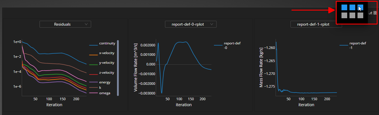
The order of the plot display can be customized to your liking by using the drop-down menu to pick and choose the plots in the corresponding window.
Hovering the mouse over the plots reveals specific data values and exposes some assorted controls for plotting:
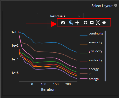
Download plot as png: saves the plot as a PNG file.
Zoom: use the mouse to draw a box that the view will zoom into.
Pan: use the mouse to pan across the XY plot.
Zoom in: zoom into the current view.
Zoom out: zoom out of the current view.
Auto-scale: resets the view to the original size and scale.
Reset Axes: resets the X and Y axes.
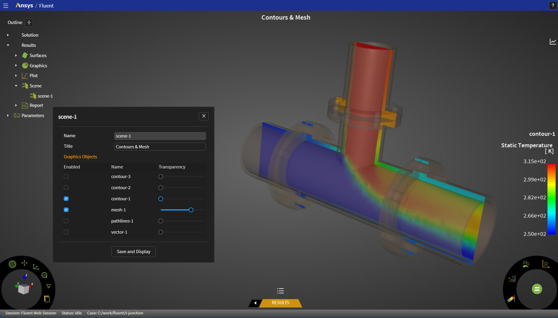
![]() Results → Scene
Results → Scene
![]() New
New
For the new scene object, open the property editor to enable/disable the display of multiple graphics plots within a single window. In the editor, you can set up different configurations of graphics results and plots from your CFD simulation. Scenes can be comprised of mesh displays, contour, vector, and pathline plots, and so forth, and the transparencies for each can be customized.
For more detailed information about scenes, see Displaying a Scene.
You can set up reports for your CFD simulation using the Outline View:
![]() Results → Reports
Results → Reports
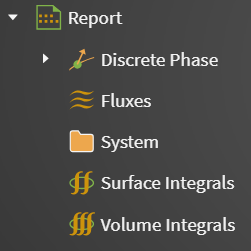
Reports can be compiled for fluxes, forces, projected areas, surface and volume integrals, among others.
- Discrete Phase
allows you to report on one of the following report types:
- Histogram
allows you to set the following:
- Histogram Options
displays options for setting up your histogram, such as whether or not to include such properties as Auto Range, Correlation, Cumulative Curve, Diameter Statistics, Histogram Mode, Percentage, Logarithmic, and Weighting.
- Histogram Parameters
displays options for setting up the number of Divisions for your histogram
For more information, see Trajectory Sample Histograms Dialog Box.
- Sample Trajectories
selecting this item opens the property editor for setting up discrete phase sample trajectories output files. For more information, see Sample Trajectories Dialog Box.
- Fluxes
selecting this item opens the property editor for fluxes where you can set up your reports for quantities such as Mass Flow, Heat Transfer, Radiation Heat Transfer, and Viscous Work. For more information, see Flux Reports Dialog Box.
- System
selecting this item opens the property editor where you can print out reports for process, system, GPGPU, and time statistics for your simulation.
- Surface Integrals
selecting this item opens the property editor for surface integrals where you can set up your reports for quantities such as Axes, Area Weighted Average, Vector Based Flux, Vector Flux, Vector Weighted Average, Facet Average, Facet Minimum, Facet Maximum, Flow Rate, Integral, Mass Flow Rate, Mass Weighted Average, Standard Deviation, Sum, Uniformity Index Area Weighted Average, Uniformity Index Mass Weighted Average, Vertex Average, Vertex Minimum, Vertex Maximum, and Volume Flow Rate. For details, see Surface Integrals Dialog Box.
- Volume Integrals
selecting this item opens the property editor for volume integrals where you can set up your reports for quantities such as Mass Average, Mass Integral, Mass, Sum, Minimum, Maximum, Volume, Volume Average, and Volume Integral. For details, see Volume Integrals Dialog Box.
For more detailed information about reports, see Reporting Alphanumeric Data.
Note: In the web interface, Fluent computes the report definitions when you click in the corresponding panel. You can generate a written report by enabling the Write to File option and clicking OK; Fluent will then prompt you for a file name and location in order to write the report.
The Parameters section of the Outline view is similar to that in Fluent, providing easy access to any of your simulation's defined input and output parameters.
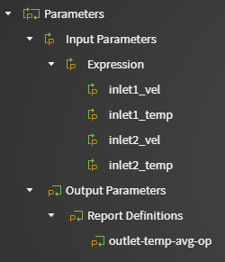
Once defined, you can quickly access input and output parameters here to view and/or change their values accordingly.