


Ansys Fluent can solve the conservation equations in a time-dependent manner, to simulate a wide variety of time-dependent phenomena, such as
vortex shedding and other time-periodic phenomena
compressible filling and emptying problems
transient heat conduction
transient chemical mixing and reactions
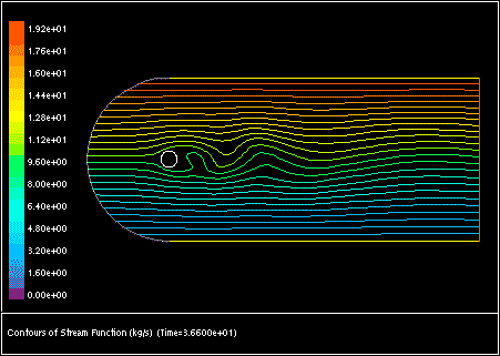
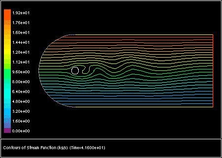
Figure 36.20: Time-Dependent Calculation of Vortex Shedding (t=36.6 sec) and Figure 36.21: Time-Dependent Calculation of Vortex Shedding (t=41.6 sec) illustrate the time-dependent vortex shedding flow pattern in the wake of a cylinder.
Enabling time dependence is sometimes useful when attempting to solve steady-state problems that tend toward instability (for example, natural convection problems in which the Rayleigh number is close to the transition region). It is possible in many cases to reach a steady-state solution by integrating the time-dependent equations.
For details about temporal discretization, see Temporal Discretization in the Theory Guide.
For additional information, see the following sections:
To solve a transient problem, you will follow the procedure outlined below:
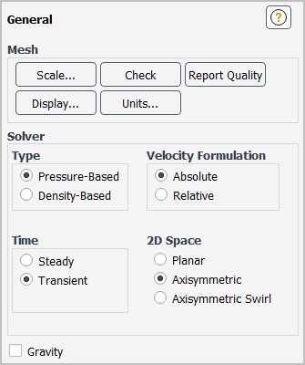
Enable the Transient option in the General task page (Figure 36.22: The General Task Page for a Transient Calculation).
 Setup →
  General
Define all relevant models and boundary conditions. Note that any boundary conditions specified using user-defined functions can be made to vary in time. See the Fluent Customization Manual for details.
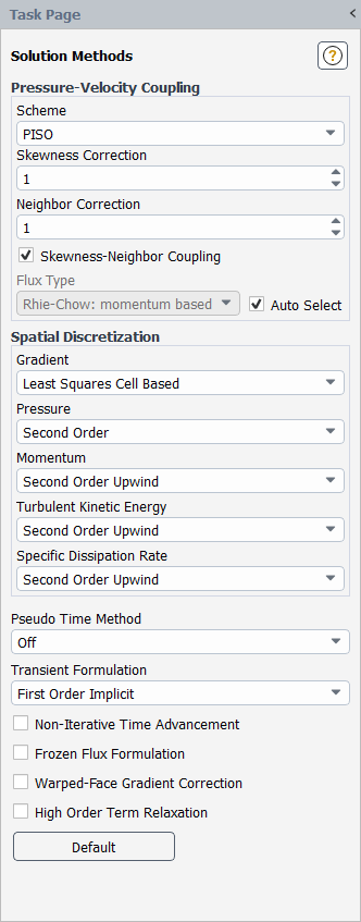
Specify the desired parameters in the Solution Methods task page (Figure 36.23: The Solution Methods Task Page for a Transient Calculation).
Solution → MethodsIf you are using the pressure-based solver, select PISO from the Scheme drop-down list in the Pressure-Velocity Coupling group box. To increase the speed of the calculations, you may need to modify the parameters related to the PISO scheme from their default values. See PISO for more information about the optimal use of the PISO algorithm.
Important:If you are using the LES turbulence model with a small time step size, the PISO scheme may be too computationally expensive. It is therefore recommended that you select SIMPLE or SIMPLEC instead of PISO.
It is best to select the Coupled pressure-velocity coupling scheme if you are using a large time step size to solve your transient flow, or if you have a poor quality mesh.
Specify the desired Transient Formulation.
The First Order Implicit formulation is sufficient for most problems. If you need improved accuracy, you can use either Second Order Implicit or Bounded Second Order Implicit. The Bounded Second Order Implicit formulation would provide better stability, since time discretization would ensure global bounds for certain variables, if available. However, note that Bounded Second Order Implicit formulation cannot ensure fully bounded solution for all variables and may result in overshoots or undershoots, especially at larger time step sizes. For cases that involve the species transport model, the population balance model, or the energy equation, you can use the below text commands to allow the first order time formulation for energy, species transport, and/or population balance equation, while retaining the second order time formulation for all other equations:
solve/set/second-order-time-optionsFor transient discretization, use variable rather than fixed time-step size formulation? [no]Allow first order time formulation for energy, species and population balance? [no]yes
Important:Note that while the Bounded Second Order Implicit formulation provides the same accuracy as the Second Order Implicit formulation, it actually provides better stability.
The Bounded Second Order Implicit formulation is available only for the pressure-based solver, and not for the density-based solver.
When using Second Order Implicit or Bounded Second Order Implicit formulation for a dynamic mesh, do not run a series of simulations in which you vary the time step size. Doing so creates an error that reduces with a reduction of the time step jump.
(density-based solver only) You can use the Explicit formulation to capture the transient behavior of moving waves, such as shocks. For details, see Temporal Discretization in the Theory Guide.
(pressure-based solver only) You have the option of using the following as part of your time-dependent flow calculations:
Non-Iterative Time Advancement (see Time-Advancement Algorithm in the Fluent Theory Guide)
Frozen Flux Formulation (see Steady-State Iterative Algorithm in the Fluent Theory Guide)
This option is only available for single-phase transient problems that do not use a moving/deforming mesh model.
Pseudo Time Method (see Performing Calculations with a Pseudo Time Method)
For transient cases, this drop-down list is only available when you have selected a segregated Scheme for the Pressure-Velocity Coupling ( SIMPLE, SIMPLEC, or PISO).
For transient cases that use the density-based explicit formulation, you can use the following text command to easily switch to a two-stage Runge-Kutta scheme for the time integration. This scheme results in faster calculations than the default three- or four-stage Runge-Kutta scheme (especially for laminar flows), though the reduced stability range may require changes to the setup as described below.
> solve/set/fast-transient-settings/rk2Enable two-stage Runge-Kutta scheme? [no]yesThis text command will set the Number of Stages to 2 in the Multi-Stage tab of the Advanced Solution Controls Dialog Box, with coefficients of 0.5 and 1. For further details about these settings, see Setting Multi-Stage Time-Stepping Parameters. If your solution diverges with this scheme, you can attempt the calculation again with a lower Courant number (typically less than 1) and, for implicit time stepping, a higher value for the maximum number of iterations per time step; if necessary, you can use the
rk2text command again to easily disable the two-stage Runge-Kutta scheme and revert back to the default multi-stage scheme for your time-stepping scheme (summarized in Summary of the Density-Based Solver in the Fluent Theory Guide).(optional) If you are using the explicit transient formulation with specified Courant number or if you are using any of the adaptive time stepping methods (described in a later step) it is recommended that you enable the printing of the current time (for the explicit transient formulation) or the current time step size (for the adaptive time stepping method) at each iteration, using Figure 36.39: Report File for 'flow-time', 'delta-time', and 'iters-per-timestep'.
Solution → Monitors →
Statistic  Edit...
Make sure that the desired item is selected from the Statistics selection list ( time for the current time or delta_time for the current time step size) and enable the Print option. When Ansys Fluent prints the residuals to the console at each iteration, it will include a column with the current time or the current time step size.
(optional) Use the Drag Report Definition Dialog Box, the Lift Report Definition Dialog Box, the Moment Report Definition Dialog Box, or the Surface Report Definition Dialog Box to monitor (and/or save to a file) time-varying force coefficient values or a report of a field variable or function on a surface as it changes with time. See Monitoring Solution Convergence for details.
Set the initial conditions (at time
 ) using the Solution Initialization task page. Solution → Initialization
You can also read in a steady-state data file to set the initial conditions.
 File → Read → Data...
Use the Autosave dialog box to specify the file name and frequency with which case and data files should be saved during the solution process. To open the Autosave dialog box, click the button next to Autosave Every in the Calculation Activities task page.
Solution → Calculation Activities →
Autosave OnSee Automatic Saving of Case and Data Files for details about automatic file saving.
The Calculation Activities task page also allows you to export solution and particle history data during the transient calculation. See Exporting Data During a Transient Calculation for details.
If you want to create a graphical animation of the solution over time, you can use Figure 36.54: The Animation Definition Dialog Box to set up the graphical displays that you want to use in the animation. See Animating the Solution for details.
You may also want to request automatic execution of other commands using the Execute Commands Dialog Box. See Executing Commands During the Calculation for details.
Specify time-dependent solution parameters and start the calculation as described below for the implicit and explicit transient formulations:
If you have chosen the First Order Implicit, Second Order Implicit, or Bounded Second Order Implicit formulation, the procedure is as follows:
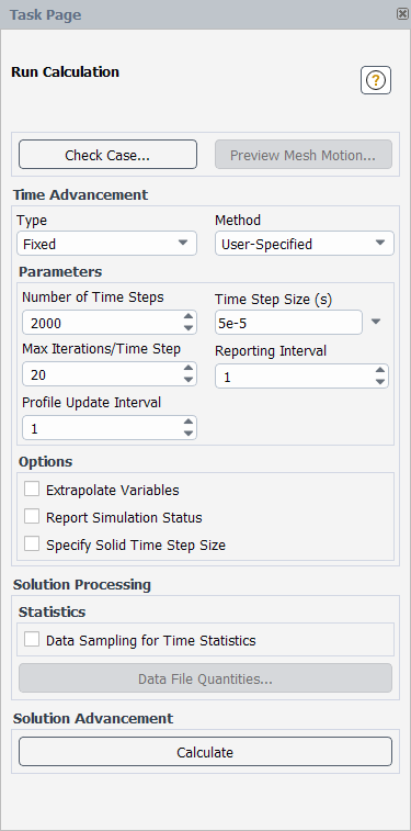
Open the Run Calculation Task Page (see Figure 36.24: The Run Calculation Task Page for Implicit Transient Calculations).
Solution → Run CalculationIf you want the time step size to remain fixed throughout the simulation, select Fixed from the Type drop-down list, and then select one of the following from the Method drop-down list:
User-Specified : with this method, you will specify the desired Number of Time Steps and the Time Step Size.
Period-Based or Frequency-Based : these methods are convenient when setting up unsteady turbomachinery cases or any case that exhibits transient periodic behavior. They allow you to define the setup in terms of the Period or Frequency, the Time Steps per Period, and the Total Periods, and then Fluent will automatically set an appropriate Time Step Size and Number of Time Steps.
When Ansys Fluent solves the time-dependent equations using the implicit formulation, multiple iterations may be necessary at each time step, so you can specify a value for the Max Iterations/Time Step you would like to allow. If the convergence criteria are met before this number of iterations is performed, the solution will advance to the next time step.
The time step size is the magnitude of
 . Since the Ansys Fluent formulation is fully implicit, there is no stability criterion that
must be met in determining
. Since the Ansys Fluent formulation is fully implicit, there is no stability criterion that
must be met in determining  . However, to model transient phenomena properly, it is necessary to set
  at least one order of magnitude smaller than the smallest time constant in the system being
modeled. A good way to judge the choice of
at least one order of magnitude smaller than the smallest time constant in the system being
modeled. A good way to judge the choice of  is to observe the number of iterations Ansys Fluent needs to converge at each time step. The
ideal number of iterations per time step is 5–10. If Ansys Fluent needs substantially more, the time step
size is too large. If Ansys Fluent needs only a few iterations per time step,
is to observe the number of iterations Ansys Fluent needs to converge at each time step. The
ideal number of iterations per time step is 5–10. If Ansys Fluent needs substantially more, the time step
size is too large. If Ansys Fluent needs only a few iterations per time step,  should be increased. Frequently a time-dependent problem has a very fast
“startup” transient that decays rapidly. Therefore, it is often wise to choose a conservatively
small
should be increased. Frequently a time-dependent problem has a very fast
“startup” transient that decays rapidly. Therefore, it is often wise to choose a conservatively
small  for the first 5–10 time steps.
  may then be gradually increased as the calculation proceeds.
For time-periodic calculations, you should choose the time step size based on the time scale of the periodicity. For a rotor/stator model, for example, you might want 20 time steps between each blade passing. For vortex shedding, you might want 20 steps per period.
To verify that your choice for
 was proper after the calculation is complete, you can plot contours of the Courant number
within the domain. To do so, select Velocity... and Cell Convective Courant
Number from the Contours of drop-down lists in the
Contours dialog box. For a stable, efficient calculation, the Courant number should not
exceed a value of 20–40 in most sensitive transient regions of the domain.
was proper after the calculation is complete, you can plot contours of the Courant number
within the domain. To do so, select Velocity... and Cell Convective Courant
Number from the Contours of drop-down lists in the
Contours dialog box. For a stable, efficient calculation, the Courant number should not
exceed a value of 20–40 in most sensitive transient regions of the domain.Note: The Period-Based and Frequency-Based methods are not available for in-cylinder dynamic mesh simulations; instead, the User-Specified method must be used, and the time step size will be computed based on the crank shaft speed and the crank angle step size.
If you want Ansys Fluent to modify the size of the time step as the calculation proceeds, select Adaptive from the Type drop-down list, and then select one of the following from the Method drop-down list:
CFL-Based: with this method, Ansys Fluent will modify the size of the time step as the calculation proceeds such that a version of the Courant–Friedrichs–Lewy (CFL) condition is satisfied. See CFL-Based Time Stepping for details.
Error-Based: with this method, the time step size is modified by Ansys Fluent based on the specified truncation Error Tolerance. See Error-Based Time Stepping for details.
Multiphase-Specific: with this method, the time step size is modified by Ansys Fluent based on the Global Courant Number. This method is available for all multiphase models using the implicit or explicit volume fraction formulation, except for the wet steam model. See Multiphase-Specific Time Stepping for details. While this method and the CFL-Based approach both use a Courant number, they differ in that the Multiphase-Specific method considers the interface regions when computing the time step size, whereas the CFL-Based method is based on a global time marching approach.
Note: The Adaptive type is not available for simulations that use the acoustic model and/or the structural model. It is also unavailable for in-cylinder dynamic mesh simulations; in this case, the fixed User-Specified method must be used, and the time step size will be computed based on the crank shaft speed and the crank angle step size.
Next, make a selection from the Duration Specification Method drop-down list in order to specify the way in which you will define the calculation duration. The duration can be defined by the total time, the total number of time steps, the incremental time, or the number of incremental time steps. In this context, "total" indicates that Fluent will consider the amount of time / steps that have already been solved and stop appropriately, whereas "incremental" indicates that the solution will proceed for a specified amount of time / steps regardless of what has previously been calculated.
It is a good idea to perform a few fixed-size time steps before switching to the adaptive time stepping. Sometimes spurious discretization errors can be associated with an impulsive start in time. These errors are dissipated during the first few time steps, but they can adversely affect the adaptive time stepping and result in extremely small time steps at the beginning of the calculation. You can specify the that should be performed before the size of the time step starts to change. The size of the fixed time step is the value specified for Initial Time Step Size ; this value must fall between the minimum and maximum time step sizes. For a better startup, it should be chosen such that the Courant number initially remains close to 1 or your specified value (whichever is lower). Note that if you initialize the solution for a previously run case with adaptive time stepping, then Ansys Fluent will use the time step size saved in the case.
Important: When the solution tends to exhibit incomplete convergence for the Error-Based method, rather than increasing the time step size or keeping the same time step size in the next step, Ansys Fluent reduces the time step size for the next time step (making sure that the time step size does not go below the specified minimum time step size).
When Ansys Fluent solves the time-dependent equations using the implicit formulation, multiple iterations may be necessary at each time step, so you can specify a value for the Max Iterations/Time Step you would like to allow. If the convergence criteria are met before this number of iterations is performed, the solution will advance to the next time step. You can also define the Time Step Size Update Interval, which specifies the number of time steps that will pass before the time step size is updated for adaptive time stepping methods.
Finally, click the button and complete the setup for the adaptive time stepping method in the Adaptive Time Stepping Dialog Box, setting the minimum / maximum time step sizes and change factors.
Tip: If you need your simulation to end exactly at your specified total or incremental time, input smaller and smaller values for the minimum time step size until this condition is met.
Note: For simulations that include automatic adaption (as described in Refining and Coarsening), the changes to the mesh during the solution may necessitate that the adaptive time step size is recalculated. For CFL-Based and Multiphase-Specific methods, this recalculated time step size is used automatically (after the completion of any initial fixed time steps). For the Error-Based method or for any adaptive method in a case with a dynamic mesh and/or sliding mesh, the recalculated time step size will not be used but will be noted in the console as a warning; if there is a large discrepancy with the time step size that is used, you should consider revising the setup to ensure time accuracy. Note that the time step size is not recalculated if the Extrapolate Variables option is enabled in the Run Calculation task page and/or if the case combines an overset mesh with the Volume of Fluid (VOF) multiphase model.
If you want to define your own adaptive time stepping method rather than use one of the Adaptive types described previously, you can create a user-defined function for your method using the
DEFINE_DELTATmacro. After you have compiled or interpreted it, you can select User-Defined Function from the Type drop-down list and then select it from the User-Defined Time Step Size drop-down list. You can then define the duration method and time / number of time steps, as described previously for the Adaptive types.See the Fluent Customization Manual for details about creating and using user-defined functions.
(optional) You can improve the convergence of the transient calculations by enabling the Extrapolate Variables option in the Run Calculation Task Page. This option instructs Ansys Fluent to predict the solution variable values for the next time step using a Taylor series expansion, and then inputs that predicted value as an initial guess for the inner iterations of the current time step. As a result, the absolute residual levels are lowered.
Note that the Extrapolate Variables option is not available if you are employing either the NITA scheme with the pressure-based solver or the explicit formulation with the density-based solver.
Important: If you use the Extrapolate Variables option when modeling an incompressible flow with the density-based solver, it is recommended that you disable the extrapolation of pressure values. After you have enabled the Extrapolate Variables option, type the following text command in the console:
> solve/set/transient-controls/extrapolate-eqn-vars/pressureExtrapolate Pressure? [yes]noTo view details about the time advancement of the simulation, enable the Report Simulation Status option in the Options group box. While this option is enabled (before, after, or during a calculation), the Simulation Status Dialog Box will be open and reporting information.
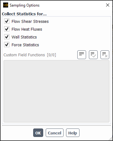
(optional) If you want Ansys Fluent to gather data for time statistics (that is, time-averaged, root-mean-square, and root-mean-square-error values for solution variables) during the calculation, you have two options for specifying the statistics that are collected during the simulation:
Use the Sampling Options Dialog Box.
Important: Statistics collected for the magnitude of a vector quantity using the Sampling Options dialog box are computed differently than those specified using the Zone-Specific Sampling Options dialog box. The former are computed as the magnitude of the mean, whereas the latter are computed as mean of the magnitude. This can lead to differences in values between the two statistics collection methods.
When you are reviewing the available variables under the Unsteady Statistics… drop-down lists during postprocessing of graphics and plot objects (contour, vector, XY plot, and so on), statistics collected based on selections in the Zone-Specific Sampling Options dialog box contain the
-datasetextension.Unsteady Statistics using the Zone-Specific Sampling Options Dialog Box
Enable the Data Sampling for Time Statistics option in the Run Calculation Task Page.
Solution → Run Calculation
→  Data Sampling for Time Statistics
Enabling this option will allow you to display and report the minimum, maximum, mean, root-mean-square-error (RMSE), moving average, and Runtime Discrete Fourier Transformation values, as described in Postprocessing for Time-Dependent Problems.
Enter a value for Sampling Interval, which is how often data samples are accumulated for computation of mean and RMS values. For example, a sampling interval of 5 means that only every 5th result is added to the statistical sampling.
The Sampled Time displays the time period over which data has been sampled for the postprocessing of the minimum, maximum, mean, root-mean-square-error (RMSE), and moving average values. For most quantities, as long as the time step size has been constant, dividing this by the time step size yields the number of data sets that have been collected. However, special consideration is required in the case of discrete phase quantities. As noted in Reporting of Unsteady DPM Statistics, sampling of DPM quantities occurs only when parcels pass through a cell, not necessarily at each specified sampling interval. Therefore, the number of samples of the DPM quantities taken during the sampled time period is stored in the separate postprocessing variable, Accum DPM Parcels in Cell. If the time step size is varied, every contribution of data sets sampled is automatically weighted by the current time step size.
Note:Input for is not applied to the runtime DFT. Accumulation of the Fourier amplitudes is done after each timestep.
Accumulation duration for the standard statistics options (minimum, maximum, mean, RMSE, moving average) may continue arbitrarily long until you stop the calculation. Differing from the standard statistics, accumulation duration for the DFT Fourier amplitudes is connected to the selected resolution of a spectrum and is fixed. Therefore, the displayed Sampling Time value may not be relevant to the runtime DFT. To estimate the DFT accumulation progress, see the value Samples to Complete for a particular DFT dataset in the Zone-Specific Sampling Options dialog box.
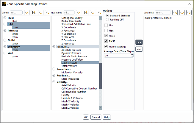
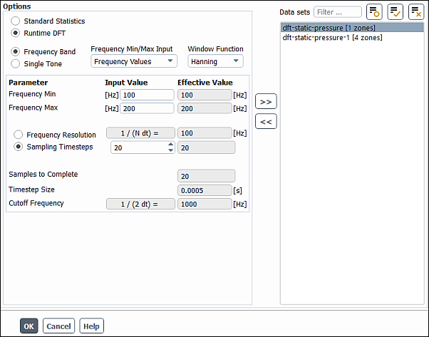
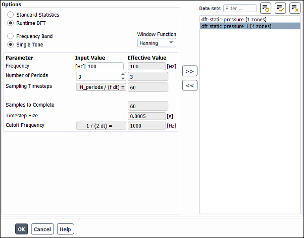
To select the quantities and locations where you want statistics collected, click the button and make selections from the Zone-Specific Sampling Options dialog box that opens (Figure 36.25: The Zone-Specific Sampling Options Dialog Box for Standard Statistics) and for Runtime DFT (Figure 36.28: Zone-Specific Sampling Options Dialog Box for Runtime DFT - Frequency Band or Figure 36.29: Zone-Specific Sampling Options Dialog Box for Runtime DFT - Single Tone).
Solution → Run Calculation
→ Sampling Options (Zone Selection)...
Important:Note that gathering data for time statistics is not meaningful inside a moving cell zone (for example, a sliding zone in a sliding mesh problem, a moving zone in a dynamic mesh problem).
Statistics are not gathered or computed on shell surfaces.
Initialize the flow statistics.
Solution → Initialization
Reset StatisticsNote that you can also reset the flow statistics after you have gathered some data for time statistics. If you perform, say, 10 time steps with the Data Sampling for Time Statistics option enabled, check the results, and then continue the calculation for 10 more time steps, the time statistics will include the data gathered in the first 10 time steps unless you reinitialize the flow statistics.
Unsteady Statistics using the Sampling Options Dialog Box
Create a custom field function for the each of the variables for which you want to postprocess unsteady statistics (for example, P*|V|), using the Custom Field Function Calculator. For detailed instructions, see Creating a Custom Field Function. Note that you do not need to take the extra step of creating custom field functions for the flow shear stresses, flow heat fluxes, wall statistics, or discrete phase variables as there are options for selecting these variables directly in a later step.
Parameters & Customization → Custom Field
Functions New...Important: The maximum number of custom field functions that can be calculated and postprocessed for unsteady statistics is 50.
Enable the Data Sampling for Time Statistics option in the Run Calculation Task Page.
Solution → Run Calculation
→ Data Sampling for Time StatisticsEnabling this option will allow you to display and report the mean, the root-mean-square (RMS), and the root-mean-square-error (RMSE) values, as described in Postprocessing for Time-Dependent Problems.
To specify the sampling interval, enter a value for Sampling Interval.
The Sampled Time displays the time period over which data has been sampled for the postprocessing of the mean, RMS, and RMSE values. For most quantities, as long as the time step size has been constant, dividing this by the time step size yields the number of data sets that have been collected. However, special consideration is required in the case of discrete phase quantities. As noted in Reporting of Unsteady DPM Statistics, sampling of DPM quantities occurs only when parcels pass through a cell, not necessarily at each specified sampling interval. Therefore, the number of samples of the DPM quantities taken during the sampled time period is stored in the separate postprocessing variable, Accum DPM Parcels in Cell. If the time step size is varied, every contribution of data sets sampled is automatically weighted by the current time step size.
To select the variables (which may be represented as custom field functions) for which you want to collect statistics, click the button and make selections from the Sampling Options dialog box that opens (Figure 36.26: The Sampling Options Dialog Box). Note that no custom field functions are selected by default.
Solution → Run Calculation
→ Sampling Options...Important: Note that gathering data for time statistics is not meaningful inside a moving cell zone (for example, a sliding zone in a sliding mesh problem, a moving zone in a dynamic mesh problem).
Initialize the flow statistics.
Solution → Initialization
Reset StatisticsNote that you can also reset the flow statistics after you have gathered some data for time statistics. If you perform, say, 10 time steps with the Data Sampling for Time Statistics option enabled, check the results, and then continue the calculation for 10 more time steps, the time statistics will include the data gathered in the first 10 time steps unless you reinitialize the flow statistics.
Click the button. As it calculates a solution, Ansys Fluent will print the current time at the end of each time step.
If you choose the Explicit transient formulation,you have two input options available for specifying the transient solution advancement: you can specify the transient advancement either directly by specifying a time step size (
 ) or indirectly via entering a Courant number value (
 ) in the Solution Controls task page. The steps for these two options are as
follows:
) in the Solution Controls task page. The steps for these two options are as
follows:If the default option Specified Time Step is enabled in the Solution Controls task page, you will be required to specify the time advancement settings in the Run Calculation task page: you need to define the time stepping as either a Fixed or User-Defined Function type (as described previously for the implicit formulations) and click the button.
Note: The stability of an explicit formulation is limited by the Courant-Fredrichs-Lewy condition. Fluent checks the specified time step size against the stability limit. The stability limit is the maximum allowable time step size calculated based on
 in Equation 36–2. The
stability limit is also the minimum of all local time steps in the domain. If the specified time step size
is larger than the maximum allowable time step, Fluent displays a warning during the calculation.
in Equation 36–2. The
stability limit is also the minimum of all local time steps in the domain. If the specified time step size
is larger than the maximum allowable time step, Fluent displays a warning during the calculation.If you disable the Specified Time Step option, you will be required to specify the Courant Number in the Solution Controls task page. Then you can define the Number of Time Steps in the Run Calculation task page and click . In this option the (
 ) value is used to calculate the time step size (
 ) using Equation 36–2 :
(36–2)
where,
 is the volume of the cell,
  is the face area, and
  is the maximum local eigenvalue defined in Equation 23–84 in the Fluent Theory Guide.
When you click the button, Ansys Fluent will begin to calculate. While the calculation is in progress, a progress bar will appear at the bottom of the Fluent window. For transient simulations, clicking the buttons next to the progress bar will interrupt the calculation at the earliest safe stopping point: you can choose to stop the calculation at the end of either the current iteration or current time step. Alternatively, you can type Ctrl+c in the console: a single instance will stop the calculation at the end of the current time step, whereas typing it twice will stop it at the end of the current iteration.
You can access the information saved in a legacy data file (that is, a
.datfile), which includes a standard set of quantities that were computed during the calculation, by clicking the button. More information about this feature is available in Setting Data File Quantities.Save the final data file (and case file, if you have modified it) so that you can continue the transient calculation later, if desired.
File → Write → Data...
The procedures for setting the reporting interval, updating user-defined function profiles and Named Expressions, interrupting iterations, and resetting data are the same as those for steady-state calculations. See Performing Steady-State Calculations for details.
Important: If you are using a user-defined function and/or named expression in your
time-dependent calculation, they will be updated after every  iterations, where
  is the value of the Profile Update
Interval (specified in the Run Calculation Task Page).
is the value of the Profile Update
Interval (specified in the Run Calculation Task Page).
As mentioned in Inputs for Time-Dependent Problems, it is possible to have the size of the time step change as the calculation proceeds such that a version of the Courant–Friedrichs–Lewy (CFL) condition is satisfied. Note that the time step size will only vary if the solution of the flow equation is enabled, and it is a convection-dominant flow. This section provides brief descriptions of the algorithms that Ansys Fluent can use to compute the time step size, as well as an explanation of parameters that you can set to control the CFL-based time stepping.
Important: CFL-based time stepping is available only with the pressure-based and density-based implicit formulations; it cannot be used
with the density-based explicit formulation. Also, it cannot be used with multiphase flows, the in-cylinder dynamic mesh option,
the acoustic model, and/or the structural model, nor is it available with the second-order implicit formulation if the fixed time
step formulation is selected through the solve/set/second-order-time-options text command or through the
enabling of a dynamic mesh.
Note: If there are other time scales controlling the physics of problem (surface tension time scale, meshing-driven time scales for mesh deformation, and so on), then the CFL-based time stepping is not a good choice.
The time step size is proportional to the defined Courant number, and can be computed considering the contribution of various time scales, such as acoustic, convective, and/or viscous time scales. By default, only the convective velocity is considered, which is suitable for low speed and incompressible flows. The time step size is calculated for each cell in the domain, and by default the minimum value is used (provided that it is within the minimum and maximum values that you have defined as part of the settings).
For transient flows, when you select Adaptive for the Type and CFL-Based for the Method in the Run Calculation task page, you can then set the time stepping parameters as described in Inputs for Time-Dependent Problems. The following provides further details that are specific for the CFL-based time stepping.
In the Run Calculation task page:
- Courant Number
is
 in Equation 36–6, which represents the ratio of the time step size to
the characteristic time taken for the fluid to cross a control volume. For convection-dominant and/or wave propagation
problems, it is recommended that you set this close to
in Equation 36–6, which represents the ratio of the time step size to
the characteristic time taken for the fluid to cross a control volume. For convection-dominant and/or wave propagation
problems, it is recommended that you set this close to 1in order to obtain more accurate results. Increasing it will result in an increase of the time step size and consequently a faster transient simulation; however, this may have a negative impact on the convergence, stability, and accuracy of your transient simulation.- Initial Time Step Size
is used for the first time step and then for as many subsequent steps as specified in the Number of Fixed Time Steps field. This value must fall between the minimum and maximum time step sizes. It should be chosen such that the Courant Number initially remains close to 1 or your specified value (whichever is lower) for a better startup. Note that if you initialize the solution for a previously run case with adaptive time stepping, then Ansys Fluent will use the time step size saved in the case file.
In the Adaptive Time Stepping dialog box (which is opened by clicking Settings... in the Run Calculation task page):
- Minimum / Maximum Step Change Factor
limit the degree to which the time step size can change at each time step. Limiting the change results in a smoother calculation of the time step size, especially when high-frequency noise is present in the solution. The time step size change factor is computed as the ratio between the current time step and the previous time step.
When choosing the values, it is generally not recommended to allow large variation in time step size due to stability considerations. This is especially true when the time step size is ramping up. It is recommended that you use a minimum time step size factor in the range of 0.5 to 0.75, and a maximum time step size change factor in the range of 1.2 to 2. The default values of 0.5 and 2, respectively, provide a smooth transition of the time step size.
If necessary, you can use the
solve/set/transient-controls/cfl-based-time-stepping-advanced-options
text command to define the following advanced settings:
You can specify whether to use the minimum CFL condition (that is, use the minimum time step calculated for all the cells in the domain) or the averaged CFL condition (in which the time step is the average value calculated for all the cells in the domain). By default the minimum CFL condition is used.
You can select the CFL type, that is, the version of the Courant–Friedrichs–Lewy (CFL) condition that is satisfied. You have the following options, and for each one a local time step size is calculated for a cell based on the Courant number (
) that you have defined as part of the settings.[1]ConvectiveFor this type, the time step size calculation is solely based on the convective velocity, according to the following formulation. This type may be more appropriate with low speed and incompressible flows, and is selected by default.

(36–3)
[2]Convective-DiffusiveFor this type, the time step size is calculated using the convective velocity contribution along with the viscous time scale, according to the following formulation. This type is recommended when viscous forces are dominant in the flow and the velocity is very small.

(36–4)
[3]AcousticFor this type, the time step size is calculated using the speed of sound rather than convective velocity according to the following formulation, and the contribution of viscous time scale is ignored. Thus, this type is recommended for supersonic compressible flows when viscous effects are not important.

(36–5)
[4]FlowFor this type, the time step size is calculated using a combination of acoustic, convective, and viscous time scales, according to the following formulation. It has been tested for various problems and is able to resolve most of the flow scales, though it may produce a less aggressive time step.
The physical eigenvalues system is considered when performing calculations with the Courant number. Eigenvalues of the system are computed based on the cell center values.

(36–6)
In the previous equations

(36–7)

(36–8)
and
 = Cell volume
 = Constant factor
 = Velocity vector for face
 = Speed of sound for face
 = Inviscid spectral radii
 = Viscous spectral radii
 = Surface area vector
 = Number of cell faces
As mentioned in Inputs for Time-Dependent Problems, it is possible to have the size of the time step change as the calculation proceeds based on the truncation error tolerance. This section provides a brief description of the algorithm that Ansys Fluent uses to compute the time step size, as well as an explanation of parameters that you can set to control the error-based time stepping.
Important: Error-based time stepping is available only with the pressure-based and density-based implicit formulations; it cannot be used with the density-based explicit formulation. It cannot be used with second-order time integration and/or the in-cylinder dynamic mesh option; it is also unavailable with Euler-Euler multiphase models (described in Approaches to Multiphase Modeling in the Theory Guide), with the exception of the Eulerian model when the implicit volume fraction formulation is enabled.
The automatic determination of the time step size is based on the estimation of the truncation error associated with the time integration scheme. If the truncation error is smaller than a specified tolerance, the size of the time step is increased; if the truncation error is greater, the time step size is decreased.
An estimation of the truncation error can be obtained by using a predictor-corrector type of algorithm [56] in association with the time integration scheme. At each time step, a predicted solution can be obtained using a computationally inexpensive explicit method: forward Euler for the first-order unsteady formulation. This predicted solution is used as an initial condition for the time step, and the correction is computed using the nonlinear iterations associated with the implicit (pressure-based or density-based) formulation. The norm of the difference between the predicted and corrected solutions is used as a measure of the truncation error. By comparing the truncation error with the desired level of accuracy (that is, the truncation error tolerance), Ansys Fluent is able to adjust the time step size by increasing it or decreasing it.
In cases where the truncation error remains above the specified tolerance, Ansys Fluent will try to meet the tolerance within
5 attempts. If this tolerance is met or the 5 attempts are completed, then the iteration moves on to the next time step. An
explicit scheme is used to predict the solution at each time step, then the explicit prediction is corrected with an implicit
scheme. The truncation error, which is a function of the difference between the predicted and corrected solutions at a specific
time is used to calculate the next time step. However, if the calculated truncation error is greater than the tolerance limit,
Ansys Fluent has the option of reverting from the currently performed iteration, which is moving from the  th step to
  th step, and performing the iteration with a smaller time step size. Since the
truncation error is proportional to the time step size, decreasing the time step size reduces the truncation error. This can be
done until the truncation error goes below the tolerance limit.
th step, and performing the iteration with a smaller time step size. Since the
truncation error is proportional to the time step size, decreasing the time step size reduces the truncation error. This can be
done until the truncation error goes below the tolerance limit.
For transient flows, when you select Adaptive for the Type and Error-Based for the Method in the Run Calculation task page, you can then set the time stepping parameters as described in Inputs for Time-Dependent Problems. The following provides further details that are specific for the error-based time stepping.
In the Run Calculation task page:
- Error Tolerance
specifies the threshold value to which the computed truncation error is compared. Increasing this value will lead to an increase in the size of the time step and a reduction in the accuracy of the solution. Decreasing it will lead to a reduction in the size of the time step and an increase in the solution accuracy, although the calculation will require more computational time. For most cases, the default value of 0.01 is acceptable.
- Initial Time Step Size
is used for the first time step and then for as many subsequent steps as specified in the Number of Fixed Time Steps field. This value must fall between the minimum and maximum time step sizes. It should be chosen such that the Courant number initially remains close to 1 for a better startup. Note that if you initialize the solution for a previously run case with adaptive time stepping, then Ansys Fluent will use the time step size saved in the case file.
In the Adaptive Time Stepping dialog box:
- Minimum/Maximum Step Change Factor
limit the degree to which the time step size can change at each time step. Limiting the change results in a smoother calculation of the time step size, especially when high-frequency noise is present in the solution. If the time step size change factor,
 , is computed as the ratio between the specified truncation error tolerance and the computed
truncation error, the size of time step
, is computed as the ratio between the specified truncation error tolerance and the computed
truncation error, the size of time step  is computed as follows:
If
 ,
,  is increased to meet the desired tolerance.
If
 ,
,  is increased, but its maximum possible value is
  .
.If
 ,
,  is unchanged.
If
 ,
,  is decreased.
Multiphase-specific time stepping is supported for all multiphase models using implicit or explicit volume fraction formulation, except for the wet steam model. It is not supported with the in-cylinder dynamic mesh option, the acoustic model, and/or the structural model.
By default, multiphase-specific time stepping is based on the convective time scale (Courant based), in which the time-step-size calculation depends on the mesh density and velocity in interfacial cells.
Note: If there are other time scales controlling the physics of problem (surface tension time scale, meshing-driven time scales for mesh deformation, and so on), then the Courant-based time scale is not a good choice.
Ansys Fluent multiphase-specific time stepping algorithm uses different time scales depending on whether physics based and moving mesh constraints are enabled or not.
Cases Without Physics Based and Moving Mesh Constraints:
Convective time scale (flux based):
 | (36–9) |
The global time step size  is calculated by:
 | (36–10) |
Cases With Physics Based and/or Moving Mesh Constraints
Based on various scales, time step sizes are defined as follows:
Convective time scale (flux based):

(36–11)
Convective time scale (velocity based):

(36–12)
Viscous time scale:

(36–13)
Gravitational time scale:

(36–14)
Surface tension driven time scale:

(36–15)
Acoustic time scale:

(36–16)
Mesh motion driven time scale (flux based):

(36–17)
Moving Mesh driven time scale (velocity based):

(36–18)
Convective time scale (aggregate):
The aggregate convective time scale is estimated by blending of flux-averaged and velocity-based time scales:

(36–19)
where the flux-averaged time scale
 is estimated by volumetric averaging of the flux-based quantities over the cell and face connected
neighbors.
is estimated by volumetric averaging of the flux-based quantities over the cell and face connected
neighbors.Moving mesh driven time scale (aggregate):
The aggregate moving mesh time scale is estimated by blending of flux-averaged and velocity-based time scales:

(36–20)
where flux-averaged time scale
 is calculated by volumetric averaging of the flux-based quantities over the cell and face connected
neighbors with non-zero mesh velocity.
is calculated by volumetric averaging of the flux-based quantities over the cell and face connected
neighbors with non-zero mesh velocity.
The effective physics based time scale is calculated as:
 | (36–21) |
The effective moving-mesh-driven time scale is calculated as:
 | (36–22) |
Global time scale  is calculated as the minimum of physics-based and moving-mesh-driven time scales for each cell:
 | (36–23) |
The above equations use the following nomenclature:
 = volume = volume |
 = outgoing relative flux due to the flow = outgoing relative flux due to the flow |
 = outgoing flux due to mesh motion = outgoing flux due to mesh motion |
 = gravity magnitude = gravity magnitude |
 = Arithmetic average of phase densities = Arithmetic average of phase densities |
 = surface tension coefficient = surface tension coefficient |
 = sound speed = sound speed |
 = maximum dynamic viscosity = maximum dynamic viscosity |
 = cell size in the direction of gravity = cell size in the direction of gravity |
 = cell size in interface normal direction = cell size in interface normal direction |
 = cell size in the direction of mesh velocity = cell size in the direction of mesh velocity |
 = averaged cell size calculated from volume = averaged cell size calculated from volume |
 = Calibration factor = 2 = Calibration factor = 2 |
 - moving mesh Courant number - moving mesh Courant number |
 - global Courant number - global Courant number |
Note: During the simulation, the Effective Global Courant Number [Multiphase Specific Time Stepping Criteria] is printed in the console. It is calculated as:

where  is the global Courant number,
  is the global time step, and
  is the effective global time step.
The effective global time step  is initiated by the global time step
  and is constrained in the following ways:

Here,
 is the previous time step, and
  and
and  are the minimum and maximum step change factors,
respectively.
are the minimum and maximum step change factors,
respectively.
Here,
 and
and  are the minimum and maximum time step sizes,
respectively.
are the minimum and maximum time step sizes,
respectively.
For transient flows, when you select Adaptive for the Type and Multiphase-Specific for the Method in the Run Calculation task page, you can then set the time stepping parameters as described in Inputs for Time-Dependent Problems. The following provides further details that are specific for the multiphase-specific time stepping.
In the Run Calculation task page:
- Global Courant Number
is the ratio of the time step size to the characteristic time taken for the fluid to cross a control volume. To calculate the Courant number, Ansys Fluent uses a flux-based definition where, in the region near the fluid interface, Ansys Fluent divides the volume of each cell by the sum of the outgoing fluxes. The resulting time represents the time it would take for the fluid to empty out of the cell. The smallest such time is used as the characteristic time of transit for a fluid element across a control volume. The default value for Global Courant Number is 2, which means that the estimated time step size is twice the characteristic time of transit.
The optimal value for Global Courant Number is dependent on a specific case. The general recommendations on choosing an appropriate value for Global Courant Number are summarized below.
Explicit volume fraction formulation
For accuracy of an instantaneous-time solution, the default value of 2 is recommended.
For a time-averaged solution, you can use higher values, but not larger than 5.
Implicit volume fraction formulation
For an instantaneous-time solution, you can set Global Courant Number to 2 (recommended) with the first order time formulation and to a higher value (up to 5) with the second order time formulation.
For a time-averaged solution, you can use even higher values (up to 20).
- Initial Time Step Size
is used for the first time step and then for as many subsequent steps as specified in the Number of Fixed Time Steps field. This value must fall between the minimum and maximum time step sizes. It should be chosen such that the Global Courant Number initially remains close to 1 or your specified value (whichever is lower) for a better startup. Note that if you initialize the solution for a previously run case with adaptive time stepping, then Ansys Fluent will use the time step size saved in the case file.
In the Adaptive Time Stepping dialog box (which is opened by clicking Settings... in the Run Calculation task page):
- Minimum / Maximum Step Change Factor
limit the degree to which the time step size can change at each time step. Limiting the change results in a smoother calculation of the time step size, especially when high-frequency noise is present in the solution. The time step size change factor is computed as the ratio between the current time step size and the previous time step size.
When choosing the values, it is generally not recommended to allow large variation in time step size due to stability considerations. This is especially true when time step size is ramping up. It is recommended that you use a minimum time step size factor in the range of 0.5 to 0.8 and a maximum time step size change factor in the range of 1.2 to 1.5. The default values of 0.8 and 1.2, respectively, provide a smooth transition of the time step size.
- Moving Mesh CFL Constraint
(VOF model only) includes moving mesh CFL constraint in the time-step-size estimation. When this option is enabled, you can adjust Moving Mesh Courant Number, which has a default value of 1. For applications with a pure rigid body motion, Moving Mesh Courant Number may not be a significant parameter.
This item is available only for applications that involve either Frame Motion, or Mesh Motion, or Dynamic Mesh. See The Multiphase-Specific Time Stepping Algorithm for details.
- Physics Based Constraint
(VOF model only) provides an option to include physics-based constraints depending on a specific type of physics involved (such as viscous, acoustic, gravitational, surface-tension-driven, and so on) in the time-step-size estimation. See The Multiphase-Specific Time Stepping Algorithm for details.
The postprocessing of time-dependent data is similar to that for steady-state data, with all graphical and alphanumeric commands available. You can read a data file that was saved at any point in the calculation (by you or with the autosave option) to restore the data at any of the time levels that were saved.
![]() File → Read → Data...
File → Read → Data...
Ansys Fluent will label any subsequent graphical or alphanumeric output with the time value of the current data set.
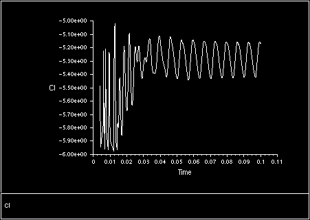
If you save data from the force or surface report definitions to files (see step 5 in Inputs for Time-Dependent Problems), you can read these files back in and plot them to see a time history of the monitored quantity. Figure 36.27: Lift Coefficient Plot for a Time-Periodic Solution shows a sample plot generated in this way.
If you enable the Data Sampling for Time Statistics option in the Run Calculation Task Page (see Performing Time-Dependent Calculations for details), Ansys Fluent will compute the time average (mean) of the instantaneous values, the root-mean-square, and the root-mean-square-errors of those quantities and custom field functions that are enabled/selected in the Sampling Options and Zone-Specific Sampling Options dialog boxes. Additionally, minimum, maximum, and runtime discrete Fourier transform (DFT) values are available if the corresponding options are enabled in the Zone-Specific Sampling Options dialog box.
The Sampled Time displays the time over which data has been sampled for the postprocessing of the mean, RMS, and RMSE values. For most quantities, as long as the time step size has been constant, dividing this by the time step size yields the number of data sets that have been collected. However, special consideration is required In the case of discrete phase quantities. As noted in Reporting of Unsteady DPM Statistics, sampling of DPM quantities occurs only when parcels pass through a cell, not necessarily at each specified sampling interval. Therefore, the number of samples of the DPM quantities taken during the sampled time period is stored in the separate postprocessing variable, Accum DPM Parcels in Cell. If the time step size is varied, every contribution of data sets sampled is automatically weighted by the current time step size.
The mean, root-mean-square(RMS), and root-mean-square-error (RMSE) values for solution variables will be available in the Unsteady Statistics... category (or the Unsteady DPM Statistics... category for discrete phase quantities) of the variable selection drop-down list that appears in postprocessing dialog boxes. For example, in the Contours dialog box, you could select Unsteady Statistics... and RMSE-uns-custom-functon-0 for the Contours of drop-down lists in order to display the root-mean-square-errors of a custom field function named uns-custom-functon-0.
The purpose of the runtime discrete Fourier transformation (DFT) in Ansys Fluent is to:
Provide spatial fields of the Fourier amplitudes and phases for postprocessing.
Create animations of the frequency-filtered transient solutions by using the Inverse DFT. Inverse DFT is a beta feature in the current version 2024 R2 and is documented in the beta features manual (Creating Animations Using Inverse DFT).
Runtime DFT is available for transient simulations and can be applied to any existing field variable. Runtime DFT is implemented as a part of the zone-specific data sampling for time statistics.
![]() Solution →
Solution → ![]() Run
Calculation → Sampling Options (Zone
Selection)
Run
Calculation → Sampling Options (Zone
Selection)
This opens the Zone-Specific Sampling Options dialog box, see Figure 36.28: Zone-Specific Sampling Options Dialog Box for Runtime DFT - Frequency Band and Figure 36.29: Zone-Specific Sampling Options Dialog Box for Runtime DFT - Single Tone. Similar to the standard zone-specific statistics, sampled DFT data are organized into datasets. Each DFT dataset contains DFT data for one quantity in one set of selected zones, for either one frequency band or one tone. If many quantities are selected at once with the same set of DFT options, then many datasets will be created, one dataset for each quantity.
The following are limitations for the Runtime DFT:
Runtime DFT is not available for the Density Based solver with the Explicit transient formulation.
Runtime DFT requires constant time stepping. The DFT datasets must be created after specifying the timestep size, because the DFT parameters are timestep-dependent. If the timestep size is changed after the dataset definition, the dataset will be removed during the calculations.
The basic mathematical formulation for the runtime DFT is provided by Equation 40–8 and Equation 40–9 in Fast Fourier Transform (FFT). To compute DFT for a non-periodic signal, the standard Hanning window function is made available:
 | (36–24) |
Note the difference between this standard Hanning window and its “tapered” modification, which is used in Ansys Fluent's FFT tool, see Equation 40–5. When the Hanning window function is used for the runtime DFT, a correction factor is applied to the accumulated Fourier amplitudes:
For a single tone dataset, an amplitude-preserving correction factor of 2 is used.
For a frequency band, an energy-preserving correction factor of
 is used.
For a frequency band, you have a choice to specify one of two values: either the band Frequency Resolution in Hz, or the number of the Sampling Timesteps. The other value is computed automatically, and your input is adjusted to the closest realizable values according to the timestep size and the frequency resolution to satisfy the following constraints:
The sampling duration is the inverse frequency step. Since the sampling duration must be a multiple of the timestep size, the user-specified frequency step is automatically adjusted to the closest realizable value.
The minimum and the maximum frequency of a band must be multiples of the frequency step. They are automatically adjusted to the closest multiples.
For a single tone, you provide the tone Frequency and the desired Number of Periods for sampling. The sampling duration is then computed using the known period size (inverse of the tone frequency). This duration is then adjusted to the closest multiple of the timestep size, and the tone frequency is adjusted accordingly, keeping the user-specified number of sampling periods. This procedure means, that with a higher number of sampling periods the needed adjustment of the user-specified tone frequency is smaller.
The following field variables are created for a DFT dataset in the Runtime DFT… category after the accumulation for a dataset is completed:
For a single tone dataset, the magnitude and the phase field variables are created. The phase is provided in radians in the range [-π, π].
For a frequency band dataset, the magnitude field variable is created. This magnitude is computed as the square root of the band power, which is the sum of the squared magnitudes of all constituent harmonics within a band.