


Piezoelectrics is the coupling of structural and electric fields, which is a natural property of materials such as quartz and ceramics. Applying a voltage to a piezoelectric material creates a displacement, and vibrating a piezoelectric material generates a voltage. A typical application of piezoelectric analysis is a pressure transducer. Possible piezoelectric analysis types are static, modal, harmonic, and transient.
Use one of these element types to perform a piezoelectric analysis:
| PLANE13, KEYOPT(1) = 7 - coupled-field quadrilateral solid |
| SOLID5, KEYOPT(1) = 0 or 3 - coupled-field brick |
| SOLID98, KEYOPT(1) = 0 or 3 - coupled-field tetrahedron |
| PLANE222, KEYOPT(1) = 1001 (charge-based) or 101 (current-based) - coupled-field 4-node quadrilateral |
| PLANE223, KEYOPT(1) = 1001 (charge-based) or 101 (current-based) - coupled-field 8-node quadrilateral |
| SOLID225, KEYOPT(1) = 1001 (charge-based) or 101 (current-based) - coupled-field 8-node brick |
| SOLID226, KEYOPT(1) = 1001 (charge-based) or 101 (current-based) - coupled-field 8-node brick |
| SOLID227, KEYOPT(1) = 1001 (charge-based) or 101 (current-based) - coupled-field 10-node tetrahedron |
| LINK228, KEYOPT(1) = 1001 (charged-based) or 101 (current-based) - coupled-field line |
The KEYOPT settings activate the piezoelectric degrees of freedom, displacements and VOLT. For SOLID5 and SOLID98, setting KEYOPT(1) = 3 activates the piezoelectric only option.
Large-deflection, stress-stiffening, and prestress effects are available (NLGEOM and PSTRES). (See the Structural Analysis Guide and Structures with Geometric Nonlinearities in the Theory Reference for more information about these capabilities.) Elements PLANE222, PLANE223, SOLID225, SOLID226, SOLID227, and LINK228 also support a linear perturbation piezoelectric analysis.
For PLANE13, large-deflection and stress-stiffening capabilities are available for KEYOPT(1) = 7. For SOLID5 and SOLID98, large-deflection and stress-stiffening capabilities are available for KEYOPT(1) = 3. In addition, small-deflection stress-stiffening capabilities are available for KEYOPT(1) = 0.
For a large-deflection piezoelectric analysis, use nonlinear-solution commands to specify your settings. For general information about the commands, refer to Setting Solution Controls in the Structural Analysis Guide.
For elements PLANE222, PLANE223, SOLID225, SOLID226, and SOLID227, KEYOPT(15) = 1 activates the piezoelectric perfectly matched layers (PML) to truncate the finite element model where the outgoing waves propagate toward infinity. Issue PMLOPT to define the normal reflection coefficients. See Example: Piezoelectric Perfectly Matched Layers for an example analysis.
The following related topics are available:
- 2.3.1. Hints and Recommendations for Piezoelectric Analysis
- 2.3.2. Material Properties for Piezoelectric Analysis
- 2.3.3. Additional Material Properties for Dynamic Piezoelectric Analysis
- 2.3.4. Example: Piezoelectric Analysis of a Bimorph
- 2.3.5. Example: Piezoelectric Analysis with Coriolis Effect
- 2.3.6. Example: Mode-Superposition Piezoelectric Analysis
- 2.3.7. Example: Piezoelectric Vibrations of a Quartz Plate
- 2.3.8. Example: Damped Vibrations of a Piezoelectric Disc
- 2.3.9. Example: Piezoelectric Perfectly Matched Layers
- 2.3.10. Other Piezoelectric Analysis Examples
The analysis may be static, modal, harmonic, or transient. For current-based piezoelectric analysis (KEYOPT(1) = 101 of PLANE222, PLANE223, SOLID225, SOLID226, SOLID227, and LINK228) the analysis must be harmonic or transient.
Some important points to remember are:
For modal analysis, Block Lanczos is the recommended solver (MODOPT,LANB). The Supernode and Subspace solvers are also allowed (MODOPT,SNODE and MODOPT,SUBSP). PCG Lanczos (MODOPT,LANPCG) is not supported unless using
Lev_Diff= 5 on PCGOPT.For damped modal analysis, the damped modal solver (MODOPT,DAMP) is recommended for low-frequency applications. The unsymmetric modal solver (MODOPT,UNSYM) is recommended for high-frequency applications. See Piezoelectrics in the Theory Reference or Table 2.11: Damping for Piezoelectric Analyses for more information about the applicable damped solvers.
For static, full harmonic, or full transient analysis, select the sparse matrix (EQSLV,SPARSE) solver or the Jacobi Conjugate Gradient (EQSLV,JCG) solver. The sparse solver is the default for static and full transient analyses. Depending on the chosen system of units or material property values, the assembled matrix may become ill-conditioned. When solving ill-conditioned matrices, the JCG iterative solver may converge to the wrong solution. The assembled matrix typically becomes ill-conditioned when the ratios of the magnitudes of the structural degree of freedom and electrical degree of freedom become very large (more than 1e15).
By default, a transient piezoelectric analysis uses
THETA= 1 for time integration (see TINTP) of the VOLT degree of freedom. Although unconditionally stable, this setting provides only first order accuracy for the electrical solution. If second order accuracy is desired, specifyALPHA= 0.25,DELTA= 0.5, andTHETA= 0.5 on the TINTP command, as described in Description of Thermal, Magnetic and Other First Order Systems in the Theory Reference.A linear perturbation piezoelectric analysis is available only with PLANE222, PLANE223, SOLID225, SOLID226, SOLID227, and LINK228 elements.
For PLANE13, SOLID5, and SOLID98, and also PLANE222, PLANE223, SOLID225, SOLID226, SOLID227, and LINK228 with KEYOPT(1) = 101, the force label for the VOLT degree of freedom is AMPS. For PLANE222, PLANE223, SOLID225, SOLID226, SOLID227, and LINK228 with KEYOPT(1) = 1001, the force label for the VOLT degree of freedom is CHRG. Use these labels in F, CNVTOL, RFORCE, etc.
To do a piezoelectric-circuit analysis, use CIRCU94. To do a current-based piezoelectric-circuit analysis, use CIRCU124.
The capability to model structural losses using the anisotropic viscosity (TB,AVIS) or the elastic loss tangent (TB,ELST) is available only for PLANE222, PLANE223, SOLID225, SOLID226, and SOLID227.
The capability to model dielectric losses using the dielectric loss tangent property (MP,LSST or TB,DLST) is available only for PLANE222, PLANE223, SOLID225, SOLID226, and SOLID227.
The capability to model resistive losses (MP,RSVX/Y/Z) is available in a transient current-based piezoelectric analysis using elements PLANE222, PLANE223, SOLID225, SOLID226, and SOLID227 with KEYOPT(1) = 101.
For the LINK228 element, dielectric loss can be modeled using the MP,LSST command only. The MP,RSVX command is available for resistive loss modeling in transient current-based piezoelectric analysis (KEYOPT(1) = 101).
The Coriolis effect capability is available only for PLANE222, PLANE223, SOLID225, SOLID226, and SOLID227. For information on how to include this effect, see Rotating Structure Analysis. For a sample analyses, see Example: Piezoelectric Analysis with Coriolis Effect.
If a model has at least one piezoelectric element, then all the coupled-field elements with structural and VOLT degrees of freedom must be of piezoelectric type. If the piezoelectric effect is not desired in these elements, simply define very small piezoelectric coefficients on TB.
Mode-superposition transient and harmonic analyses (see Performing a Mode-Superposition Transient Dynamic Analysis and Mode-Superposition Harmonic Analysis in the Structural Analysis Guide) are available with the following conditions:
For voltage excitation (D,,VOLT), use the enforced motion procedure. For an example, see Example: Mode-Superposition Piezoelectric Analysis.
For electric charge excitation (F,,CHRG, SF,,CHRGS, or BF,,CHRGD), create a load vector during the modal analysis and scale it during the mode-superposition analysis (LVSCALE). The residual response method is strongly recommended for electric charge excitation.
Use a sufficient number of modes to obtain an accurate voltage solution. The upper frequency times two for the modal base may be insufficient. In general, as the number of modes increases, the convergence of the voltage solution is slower than the convergence of the displacement solution, especially far from the resonance frequencies.
Mode-superposition analysis does not support the following forms of damping: electrical resistivity (MP,RSVX, RSVY and RSVZ), electric loss tangent (MP,LSST), and anisotropic dielectric loss tangent (TB,DLST). For more information, see Table 2.11: Damping for Piezoelectric Analyses and Damping in the Structural Analysis Guide.
If you are interested in results such as electric fields (
Item= EF on PRNSOL, PLNSOL, PRESOL, or PLESOL) or charges (Item= CHRG on PRESOL or PLESOL), request an expansion which is not based on modal elements results by specifyingMSUPkey= NO on MXPAND.Prestressed mode-superposition piezoelectric analysis is also available using the linear perturbation modal analysis. For more details, see Linear Perturbation Analysis in the Structural Analysis Guide.
A piezoelectric model requires permittivity (or dielectric constants), the piezoelectric matrix, and the elastic coefficient matrix to be specified as material properties. See the following topics for details:
For SOLID5, PLANE13, or SOLID98 you specify relative permittivity values as PERX, PERY, and PERZ on MP (). (See EMUNIT for information on free-space permittivity.) The permittivity values represent the diagonal components ε11, ε22, and ε33 respectively of the permittivity matrix [εS]. (The superscript "S" indicates that the constants are evaluated at constant strain.) That is, the permittivity input on MP is always interpreted as permittivity at constant strain [εS].
Note: If you enter permittivity values less than 1 for SOLID5, PLANE13, or SOLID98, the program interprets the values as absolute permittivity.
For PLANE222,
PLANE223, SOLID225,
SOLID226, and SOLID227,
you can specify permittivity either as PERX, PERY, PERZ on MP
or by specifying the terms of the anisotropic permittivity matrix via
TB,DPER and TBDATA. If you use
MP to specify permittivity, the permittivity input is
interpreted as permittivity at constant strain. If you use
TB,DPER (), you can specify the permittivity matrix at constant
strain [εS] (TBOPT
= 0) or at constant stress [εT]
(TBOPT = 1). The latter input will be internally
converted to permittivity at constant strain
[εS] using the piezoelectric strain and
stress matrices. The values input on either MP,PERX or
TB,DPER are always interpreted as relative
permittivity.
For LINK228, you specify relative permittivity values as PERX on MP. The permittivity input is interpreted as permittivity at constant strain.
You can define the piezoelectric matrix in [e] form (piezoelectric stress matrix) or in [d] form (piezoelectric strain matrix). The [e] matrix is typically associated with the input of the anisotropic elasticity in the form of the stiffness matrix [c], while the [d] matrix is associated with the compliance matrix [s].
Note: The program converts a piezoelectric strain matrix [d] matrix to a piezoelectric stress matrix [e] using the elastic matrix at the first defined temperature. To specify the elastic matrix required for this conversion, issue TB,ANEL (not MP).
This 6 x 3 matrix (4 x 2 for 2D models) relates the electric field to stress ([e] matrix) or to strain ([d] matrix). Both the [e] and the [d] matrices use the data table input described below:

TB,PIEZ and TBDATA define the piezoelectric matrix.
The LINK228 element uses the axial component of the piezoelectric matrix only (e11).
To define the piezoelectric matrix via the GUI, use the following:
For most published piezoelectric materials, the order used for the piezoelectric matrix is x, y, z, yz, xz, xy, based on IEEE standards (see ANSI/IEEE Standard 176–1987), while the input order is x, y, z, xy, yz, xz as shown above. This means that you need to transform the matrix to the input order by switching row data for the shear terms as shown below:
IEEE constants [e61, e62, e63] would be input as the xy row
IEEE constants [e41, e42, e43] would be input as the yz row
IEEE constants [e51, e52, e53] would be input as the xz row
This 6 x 6 symmetric matrix (4 x 4 for 2D models) specifies the stiffness ([c] matrix) or compliance ([s] matrix) coefficients.
Note: This section follows the IEEE standard notation for the elastic coefficient matrix [c]. The matrix is also referred to as [D].
The elastic coefficient matrix uses the following data table input:

Issue TB,ANEL () and TBDATA to define the coefficient matrix [c] (or [s], depending on the TBOPT settings). As for the piezoelectric matrix, most published piezoelectric materials use a different order for the [c] matrix. Transform the IEEE matrix to the input order by switching row and column data for the shear terms, as shown:
IEEE terms [c61, c62, c63, c66] would be input as the xy row
IEEE terms [c41, c42, c43, c46, c44] would be input as the yz row
IEEE terms [c51, c52, c53, c56, c54, c55] would be input as the xz row
An alternative to the [c] matrix is to specify Young's modulus (MP,EX) and Poisson's ratio (MP,NUXY) and/or shear modulus (MP,GXY). For LINK228, this method is recommended, and Young’s modulus (MP,EX) is the only effective material property.
To specify any of these via the GUI, use the following:
For micro-electromechanical systems (MEMS), it is best to set up problems in µMKSV or µMSVfA units (see Table 1.7: Piezoelectric Conversion Factors for MKS to μMKSV and Table 1.14: Piezoelectric Conversion Factors for MKS to μMKSVfA).
For PLANE222, PLANE223, SOLID225, SOLID226, and SOLID227, elastic, piezoelectric, and permittivity matrix coefficients can be functions of primary variables via tabular input. You can use this capability to specify temperature-dependent or frequency-dependent matrix coefficients, as described below for the case of temperature dependent properties:
For each temperature-dependent coefficient, issue this command to declare and dimension the table array parameter
Parwith the TEMP primary variable:*DIM, Par,TABLE,,,,TEMPFor each temperature-dependent coefficient, define the temperature dependence by specifying the table array values. Various ways of specifying the array entries are described in Specifying Array Element Values in the Ansys Parametric Design Language Guide.
Define the table for the specific material (TB,ANEL for elastic, TB,PIEZ for piezoelectric, or TB,DPER for dielectric permittivity) with
TBOPT= 0.Input the coefficients using TBDATA. For those coefficients defined by tabular input, enclose the table array parameter name within % characters:
TBDATA, STLOC,%Par%
Example 2.1: Using Tabular Input (via TBDATA) to Define Temperature-Dependence
In this example, temperature-dependence is specified for the piezoelectric coefficients e11 and e14 of quartz.
! Piezoelectric stress constants (C/m**2) and
! their temperature coefficients (1/deg.C)
e11= 0.171    $ Te11= -1.6e-4
e14=-0.0406   $ Te14= -14.4e-4

! Piezoelectric coefficients at T = 0 deg. C
e11_0=e11*(1+Te11*(0-25))
e14_0=e14*(1+Te14*(0-25))

! Piezoelectric coefficients at T = 100 deg. C
e11_100=e11*(1+Te11*(100-25))
e14_100=e14*(1+Te14*(100-25))

*dim,e11_T,table,2,,,temp
e11_T(1,0)= 0,100              ! temperature range
e11_T(1,1)= e11_0,e11_100      ! e11(t)

*dim,ne11_T,table,2,,,temp
ne11_T(1,0)= 0,100             ! temperature range
ne11_T(1,1)= -e11_0,-e11_100   ! -e11(t)

*dim,e14_T,table,2,,,temp
e14_T(1,0)= 0,100              ! temperature range
e14_T(1,1)= e14_0,e14_100      ! e14(t)

*dim,ne14_T,table,2,,,temp
ne14_T(1,0)= 0,100             ! temperature range
ne14_T(1,1)= -e14_0,-e14_100   ! -e14(t)

tb,PIEZ,1,,,0                  ! Piezoelectric table
tbda,1,%e11_T%                 ! [ e11  0  0]
tbda,4,%ne11_T%                ! [-e11  0  0]
tbda,7                         ! [  0   0  0]
tbda,10,,%ne11_T%              ! [  0 -e11 0]
tbda,13,%e14_T%                ! [ e14  0  0]
tbda,16,,%ne14_T%              ! [  0 -e14 0]
For more information, see Defining Linear Material Properties Using Tabular Input in the Material Reference.
In addition to electrical permittivity, the piezoelectric matrix, and the elastic coefficient matrix, a dynamic piezoelectric analysis (modal, harmonic, transient, or linear perturbation harmonic and modal) requires density (MP,DENS) to be specified as material property.
Structural losses can be accounted for by specifying material damping properties. (See Material-Dependent Alpha and Beta Damping (Rayleigh Damping) and Material-Dependent Structural Damping in the Material Reference.)
For PLANE222, PLANE223, SOLID225, SOLID226, and SOLID227, you can also specify anisotropic structural damping in the form of:
Anisotropic viscosity (TB,AVIS) (in harmonic and transient analyses)
Anisotropic elastic loss tangent (TB,ELST) (in a harmonic analysis)
For the same elements, you can specify the following electrical losses:
Electrical resistivity (MP,RSVX/Y/Z) in a transient current-based analysis
Dielectric loss tangent (MP,LSST) in charge-based harmonic and modal analyses
Anisotropic dielectric loss tangent (TB,DLST) in charge-based harmonic and modal analyses
For LINK228, you can specify the following electrical losses:
The anisotropic material properties are not supported by the LINK228 element.
The following table summarizes the different types of damping that are supported in dynamic piezoelectric analyses (For detailed equations and underlying theory, see Losses in a Piezoelectric Analysis in the Theory Reference).
Table 2.11: Damping for Piezoelectric Analyses
| Loss | Analysis Type | |||||
|---|---|---|---|---|---|---|
| Type | Input | Modal | Full Harmonic | Full Transient | ||
| DAMP | UNSYM | QRDAMP[a] | ||||
| Structural | MP,BETD[b] | x | x | x | x | |
| TB,AVIS | x | x | x | x | ||
| MP,DMPR[b] | x | x | x | x | ||
| MP,DMPS[b] | x | x | x | x | ||
| TB,SDAMP | x | x | x | x | ||
| TB,ELST | x | x | x | x | ||
| Electrical | MP,LSST[b] | x | x | x | x | |
| TB,DLST | x | x | x | x | ||
| MP,RSVX[b]/Y/Z | x | x[c] | ||||
[a] Structural damping types are also supported in QR-Damped mode-superposition analyses and linear perturbation mode-superpostion analyses. (See Mode-Superposition Harmonic Analysis, Performing a Mode-Superposition Transient Dynamic Analysis, and Linear Perturbation Analysis in the Structural Analysis Guide.)
[c] The transient analysis must be a current-based piezoelectric analysis (KEYOPT(1) = 101).
This example problem considers a piezoelectric bimorph beam in actuating and sensing modes.
The following topics are available:
A piezoelectric bimorph beam is composed of two piezoelectric layers joined together with opposite polarities. Piezoelectric bimorphs are widely used for actuation and sensing. In the actuation mode, on the application of an electric field across the beam thickness, one layer contracts while the other expands. This results in the bending of the entire structure and tip deflection. In the sensing mode, the bimorph is used to measure an external load by monitoring the piezoelectrically induced electrode voltages.
As shown in Figure 2.10: Piezoelectric Bimorph Beam, this is a 2D analysis of a bimorph mounted as a cantilever. The top surface has ten identical electrode patches and the bottom surface is grounded.
In the actuator simulation, perform a linear static analysis. For an applied voltage of 100 Volts along the top surface, determine the beam tip deflection. In the sensor simulation, perform a large-deflection static analysis. For an applied beam tip deflection of 10 mm, determine the electrode voltages (V1, V2, ... V10) along the beam.

The bimorph material is Polyvinylidene Fluoride (PVDF) with the following properties:
| Young's modulus (E1) = 2.0e9 N/m2 |
| Poisson's ratio (ν12) = 0.29 |
| Shear modulus (G12) = 0.775e9 N/m2 |
| Piezoelectric strain coefficients (d31) = 2.2e-11 C/N, (d32) = 0.3e-11 C/N, and (d33) = -3.0e-11 C/N |
| Relative permittivity at constant stress (ε33)T = 12 |
The geometric properties are:
| Beam length (L) = 100 mm |
| Layer thickness (H) = 0.5 mm |
Loadings for this problem are:
| Electrode voltage for the actuator mode (V) = 100 Volts |
| Beam tip deflection for the sensor mode (Uy) = 10 mm |
Actuator Mode
A deflection of -32.9 µm is calculated for 100 Volts.
This deflection is close to the theoretical solution determined by the following formula (J.G. Smits, S.I. Dalke, and T.K. Cooney, "The constituent equations of piezoelectric bimorphs," Sensors and Actuators A, 28, pp. 41–61, 1991):
Uy = -3(d31)(V)(L)2/8(H)2
Substituting the problem values gives a theoretical deflection of -33.0 µm.
Sensor Mode
Electrode voltage results for a 10 millimeter beam tip deflection are shown in Table 2.12: Electrode 1-5 Voltages and Table 2.13: Electrode 6-10 Voltages. They are in good agreement with those reported by W.-S. Hwang and H.C. Park ("Finite Element Modeling of Piezoelectric Sensors and Actuators," American Institute of Aeronautics and Astronautics, Vol. 31, No.5, pp. 930-937, 1993).
The command listing below demonstrates the problem input. Text prefaced by an exclamation point (!) is a comment. An alternative element type and material input are included in the comment lines.
/batch,list
/title, Static Analysis of a Piezoelectric Bimorph Beam
/nopr
/com,
/PREP7
!
!  Define problem parameters
!
!   - Geometry
!
L=100e-3                        ! Length, m
H=0.5e-3                        ! One-layer thickness, m
!
!   - Loading
!
V=100                           ! Electrode voltage, Volt
Uy=10.e-3                       ! Tip displacement, m
!
!   - Material properties for PVDF
!
E1=2.0e9                        ! Young's modulus, N/m^2
NU12=0.29                       ! Poisson's ratio
G12=0.775e9                     ! Shear modulus, N/m^2
d31=2.2e-11                     ! Piezoelectric strain coefficients, C/N
d32=0.3e-11
d33=-3.0e-11
ept33=12                        ! Relative permittivity at constant stress
!
! Finite element model of the piezoelectric bimorph beam
!
local,11                        ! Coord. system for lower layer: polar axis +Y
local,12,,,,,180                ! Coord. system for upper layer: polar axis -Y
csys,11                         ! Activate coord. system 11
rect,0,L,-H,0                   ! Create area for lower layer
rect,0,L, 0,H                   ! Create area for upper layer
aglue,all                       ! Glue layers
esize,H                         ! Specify the element length
!
et,1,PLANE223,1001,,0           ! 2D piezoelectric element, plane stress

tb,ANEL,1,,,1                  ! Elastic compliance matrix
tbda,1,1/E1,-NU12/E1,-NU12/E1
tbda,7,1/E1,-NU12/E1
tbda,12,1/E1
tbda,16,1/G12

tb,PIEZ,1,,,1                   ! Piezoelectric strain matrix
tbda,2,d31
tbda,5,d33
tbda,8,d32

tb,DPER,1,,,1                   ! Permittivity at constant stress
tbdata,1,ept33,ept33

tblist,all                      ! List input and converted material matrices

! -------------------------------------------------------------------------
!          Alternative element type and material input
!
!et,1,PLANE13,7,,2               ! 2D piezoelectric element, plane stress
!
!mp,EX,1,E1                      ! Elastic properties
!mp,NUXY,1,NU12
!mp,GXY,1,G12
!
!tb,PIEZ,1                       ! Piezoelectric stress matrix
!tbda,2,0.2876e-1
!tbda,5,-0.5186e-1
!tbda,8,-0.7014e-3
!
!mp,PERX,1,11.75                 ! Permittivity at constant strain
! -------------------------------------------------------------------------
type,1 $ esys,11
amesh,1                         ! Generate mesh within the lower layer
type,1 $ esys,12
amesh,3                         ! Generate mesh within the upper layer
!
nsel,s,loc,x,L
*get,ntip,node,0,num,min        ! Get master node at beam tip
!
nelec = 10                      ! Number of electrodes on top surface
*dim,ntop,array,nelec
l1 = 0                          ! Initialize electrode locations
l2 = L/nelec
*do,i,1,nelec                   ! Define electrodes on top surface
nsel,s,loc,y,H
nsel,r,loc,x,l1,l2
cp,i,volt,all
*get,ntop(i),node,0,num,min     ! Get master node on top electrode
l1 = l2 + H/10                  ! Update electrode location
l2 = l2 + L/nelec
*enddo
nsel,s,loc,y,-H                 ! Define bottom electrode
d,all,volt,0                    ! Ground bottom electrode
nsel,s,loc,x,0                  ! Clamp left end of bimorph
d,all,ux,0,,,,uy
nsel,all
fini
/SOLU                           ! Actuator simulation
antype,static                   ! Static analysis
*do,i,1,nelec
d,ntop(i),volt,V                ! Apply voltages to top electrodes
*enddo
solve
Uy_an = -3*d31*V*L**2/(8*H**2)  ! Theoretical solution
/com,
/com, Actuator mode results:
/com, - Calculated tip displacement Uy = %uy(ntip)% (m)
/com, - Theoretical solution        Uy = %Uy_an% (m)
fini
/SOLU                           ! Sensor simulation
antype,static,new
*do,i,1,nelec
ddele,ntop(i),volt              ! Delete applied voltages
*enddo
d,ntip,uy,Uy                    ! Apply displacement to beam tip
nlgeom,on                       ! Activate large deflections
nsubs,2                         ! Set number of substeps
cnvtol,F,1.e-3,1.e-3            ! Set convergence for force
cnvtol,CHRG,1.e-8,1.e-3         ! Set convergence for charge
!cnvtol,AMPS,1.e-8,1.e-3         ! Use AMPS label with PLANE13
solve
fini
/POST1
/com,
/com, Sensor mode results:
*do,i,1,nelec
/com, - Electrode %i%  Voltage = %volt(ntop(i))% (Volt)
*enddo
/com,
/view,,1,,1                     ! Set viewing directions
/dscale,1,1                     ! Set scaling options
pldisp,1                        ! Display deflected and undeflected shapes
path,position,2,,100            ! Define path name and parameters
ppath,1,,0,H                    ! Define path along bimorph length
ppath,2,,L,H
pdef,Volt,volt,,noav            ! Interpolate voltage onto the path
pdef,Uy,u,y                     ! Interpolate displacement onto the path
/axlab,x, Position (m)
/axlab,y, Electrode Voltage (Volt)
plpath,Volt                     ! Display electrode voltage along the path
/axlab,y, Beam Deflection (m)
plpath,Uy                       ! Display beam deflection along the path
pasave                          ! Save path in a file
fini
This example demonstrates a piezoelectric analysis with Coriolis effect in a rotating reference frame.
The following topics are available:
A quartz tuning fork for an angular velocity sensor consists of two tines connected to a base that is fixed at the bottom. SOLID226 elements model the tuning fork as shown in the following figure.
The tuning fork is excited into an in-plane vibration by an applied alternating voltage. When the tuning fork is rotated about the axis parallel to the tines (Y-axis) with an angular velocity Ω, the Coriolis effect produces a torque proportional to Ω. Converted to an electric output signal, the amplitude of the out-of-plane vibration can be used to sense the rotational velocity in angular velocity sensors.
An undamped modal analysis (MODOPT,LANB) is first performed to determine the eigenfrequencies of a tuning fork without inertia effects. It is followed by a damped modal analysis (MODOPT,DAMP) of the rotating tuning fork to determine the shift in the eigenfrequencies due to Coriolis and spin-softening effects. The Coriolis effect is activated in a rotating reference frame via CORIOLIS,ON,,,OFF. Angular velocity is specified via OMEGA.
A harmonic analysis is also performed to demonstrate the effect of Coriolis force in the vicinity of the 4th resonance.
Geometric and material properties are input in the μMKSV system of units. For more information on units, see System of Units.
The tuning fork dimensions are:
| Thickness (T) = 350 μm |
| Tine width (W_t) = 450 μm |
| Base width (W) = 1250 μm |
| Tine length (L_t) = 3200 μm |
| Total length (L) = 4800 μm |
Material property inputs for quartz are: elastic coefficients, piezoelectric coefficients, dielectric constants, and density (Bechmann, R., "Elastic and Piezoelectric Constants of Alpha-Quartz," Physical Review, v.110, pp. 1060-1061 (1958)).
The operating parameters are:
| Angular velocity (Ω) = 1e4 rad/s (Ω is typically around 1 rad/s for gyroscopes. It is greatly exaggerated here to show the out-of-plane motion in the animation.) |
| Operating frequency (f) = 32768 Hz (This frequency corresponds to a quartz clock. Gyroscopes can operate at a different frequency.) |
Eigenfrequencies are shown in the following table. Spin-softening effects are included by default in dynamic analyses when the Coriolis effect is enabled (CORIOLIS,ON).
Table 2.14: Tuning Fork Eigenfrequencies (Hz)
| Mode | No Inertia Effects | Coriolis Effect and Spin-Softening |
|---|---|---|
| 1st | 15095 | 14904 |
| 2nd | 24052 | 23765 |
| 3rd | 30129 | 30303 |
| 4th | 32736 | 33020 |
To expand the corresponding complex mode shapes, set the
Cpxmod argument on MODOPT to
ON and issue MXPAND.
The in-plane and out-of-plane vibrations in the vicinity of the 4th resonance are shown in the following animation. View the animation online if you are reading the PDF version of the help.
The command listing below demonstrates the problem input. Text prefaced by an exclamation point (!) is a comment.
title, Coriolis Effect in a Vibrating Quartz Tuning Fork
/com  uMKS system of units
/nopr

pi  = 4*atan(1)
/VIEW,1,1,1,1
/TRIAD,lbot

/PREP7
! == Material parameters
! -- Elastic coefficients, MPa
c11      = 86.74e3
c12      = 6.99e3
c13      = 11.91e3
c14      = 17.91e3
c33      = 107.2e3
c44      = 57.94e3
tb,ANEL,1
tbdata, 1,  c11, c12, c13,    0, c14,    0
tbdata, 7,       c11, c13,    0,-c14,    0
tbdata,12,            c33,    0,   0,    0
tbdata,16,          (c11-c12)/2,   0,  c14
tbdata,19,                       c44,    0
tbdata,21,                             c44

! -- Piezoelectric coefficients, pC/um2
e11 = 0.171
e14 =-0.0406
tb,PIEZ,1
tbdata, 1,  e11,    0,   0
tbdata, 4, -e11,    0,   0
tbdata, 7,    0,    0,   0
tbdata,10,    0, -e11,   0
tbdata,13,  e14,    0,   0
tbdata,16,    0, -e14,   0

! -- Dielectric constants
emunit,EPZRO,8.854e-6             ! pF/um
mp,PERx,1, 4.43
mp,PERy,1, 4.43
mp,PERz,1, 4.63

! -- Density, kg/um3
mp,DENS,1,2649e-18

! == Dimensions, um

thick    =  350                   ! thickness of wafer
leng_TF  = 4800                   ! length of tuning fork
leng_tin = 3200                   ! length of tines
dist_t   =  350                   ! distance between tines
width_t  =  450                   ! width of tines
x_t_in   = dist_t/2               ! distance to outer part of tines
x_t_out  = dist_t/2 + width_t     ! distance to inner part of tines

! == FE Model

et,1,SOLID226,1001                ! piezoelectric 20-node brick

! -- Keypoints
k, 1, 0,       0                , -thick/2
k, 2, 0,       leng_TF-leng_tin , -thick/2
k, 3, x_t_in,  0                , -thick/2
k, 4, x_t_in,  leng_TF-leng_tin , -thick/2
k, 5, x_t_in,  leng_TF          , -thick/2
k, 6, x_t_out, 0                , -thick/2
k, 7, x_t_out, leng_TF-leng_tin , -thick/2
k, 8, x_t_out, leng_TF          , -thick/2

! -- Areas
a,1,3,4,2
a,3,6,7,4
a,4,7,8,5

! -- Lines
lesize, 5,,,  4,                  ! X, tines
*repeat,3,2
lesize, 1,,,  2,                  ! X, between tines
lesize, 3,,,  2,
lesize, 8,,, 14,  3               ! Y, tines
lesize,10,,, 14, 1/3
lesize, 2,,, 8, -2                ! Y, base
*repeat,3,2
*get,n_lin,LINE,,count            ! number of lines
lgen,2,1, n_lin, 1,,, thick,20    ! generate top layer lines
l,1,21, 4,                        ! thickness direction
*repeat,8,1,1

lsymm,X,all,,,100                 ! generate left half of tuning fork

! -- Volumes
v,  1,  3,  4,  2,  21, 23, 24, 22
v,  3,  6,  7,  4,  23, 26, 27, 24
v,  4,  7,  8,  5,  24, 27, 28, 25
v,101,103,104,102, 121,123,124,122
v,103,106,107,104, 123,126,127,124
v,104,107,108,105, 124,127,128,125
vplot
nummrg,kp

! -- Mesh
type,1
vmesh,all

! == Define electrodes
delta=20                         ! separation between electrodes and edge

! -- Loaded electrode
nsel,s,loc,x, x_t_in+delta, x_t_out-delta     ! top/bottom right tine
nsel,u,loc,z, -thick/2+1, thick/2-1
nsel,a,loc,x, -x_t_out-1, -x_t_out+1          ! sides of left tine
nsel,a,loc,x, -x_t_in-1,  -x_t_in+1
nsel,r,loc,y, leng_TF-leng_tin-1, leng_TF-leng_tin*0.45  ! select tine-nodes
cp,1,volt,all
n_load=ndnext(0)                 ! get master node on loaded electrode

! -- Ground electrode
nsel,s,loc,x, -x_t_out+delta, -x_t_in-delta   ! top/bottom left tine
nsel,u,loc,z, -thick/2+1, thick/2-1
nsel,a,loc,x, x_t_out-1, x_t_out+1            ! sides of right tine
nsel,a,loc,x, x_t_in-1,  x_t_in+1
nsel,r,loc,y, leng_TF-leng_tin-1, leng_TF-leng_tin*0.45  ! select tine-nodes
cp,2,volt,all
n_ground=ndnext(0)               ! get master node on ground electrode
nsel,all

! == Solution
/SOLU
! -- Structural constraints
nsel,s,loc,y
d,all,ux,0,,,,uy,uz
nsel,all

! -- Ground electrode
d,n_ground,volt,0                ! ground
! -- Loaded electrode
d,n_load,volt,1                  ! apply 1 Volt

fini

! == Undamped modal analysis
/SOLU
antype,modal
modopt,LANB,4                  ! use block Lanczos eigensolver
solve
fini

! == Damped modal analysis
/SOLU
antype,modal
coriolis,on,,,off              ! Coriolis effect in a rotating reference frame
omega,,1.e4                    ! rotational velocity about the Y axis, rad/s
modopt,DAMP,8                  ! use damped eigensolver
solve
fini

! == Harmonic analysis
/SOLU
antype,harm
dmpstr,0.04                    ! specify structural damping coefficient
harfrq,,32768
outres,all,all
solve
fini

/POST1
set,1,1
/dscale,1,6
plns,u,z
anharm                         ! animate complex displacements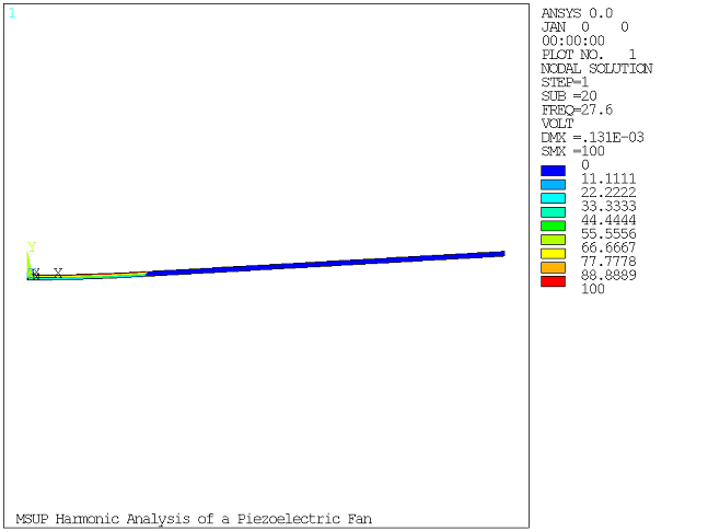
finiThis example problems considers a simplified model of a piezoelectric fan to demonstrate the mode-superposition harmonic procedure.
The following topics are available:
A piezoelectric bimorph beam is considered, as in Example: Piezoelectric Analysis of a Bimorph. For a specific description of the beam, see Problem Description. In this example, the beam is a cantilever and only one fourth of its length has piezoelectric characteristics. The rest is a purely structural flexible beam which amplifies the piezoelectric motion.
As voltage is applied along the upper layer of the piezoelectric part, the beam oscillates and generates airflow.
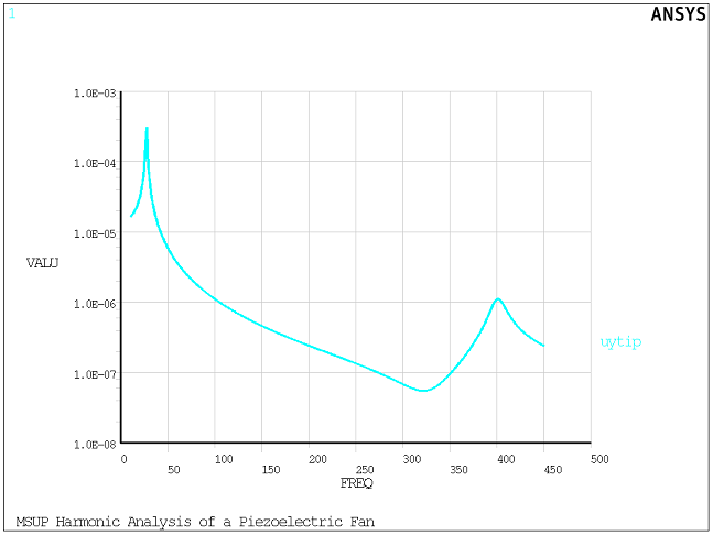
A mode-superposition harmonic analysis is performed to obtain the amplitude of vibration as a function of the alternating current frequency.
The biomorph material is Polyvinylidene Fluoride (PVDF) with the following properties:
| Young’s modulus (E1) = 2.0 x 10⁹ N/m2 |
| Poisson’s ratio (v12) = 0.29 |
| Shear modulus (G12) = 0.775 x 10⁹ N/m2 |
| Piezoelectric strain coefficients (d31) = 2.2 x 10⁻¹¹ C/N, (d32) = 0.3 x 10⁻¹¹ C/N, and (d33) = -3.0 x 10⁻¹¹ C/N |
| Relative permittivity at constant stress (ε33)T = 12 |
The geometric properties are:
| Beam length (L) = 100 mm |
| Layer thickness (H) = 0.5 mm |
The loading for this problem is:
| Electrode voltage = 100 Volts |
The volt solution and the animation of the vibration in the vicinity of the 1st resonance frequency are shown in the following figures. View the animation online if you are using the PDF version of this document.
The evolution of the tip deflection with respect to the frequency is shown below.
The command text below demonstrates the problem input. All text prefaced with an exclamation point (!) is a comment.
/title, MSUP Harmonic Analysis of a Piezoelectric Fan
/PREP7
!
!   - Geometry
!
L=100e-3                        ! Length, m
H=0.5e-3                        ! One-layer thickness, m
!
!   - Loading
!
V=100                           ! Electrode voltage, Volt
!
!   - Material properties for PVDF
!
E1=2.0e9                        ! Young's modulus, N/m^2
NU12=0.29                       ! Poisson's ratio
G12=0.775e9                     ! Shear modulus, N/m^2
d31=2.2e-11                     ! Piezoelectric strain coefficients, C/N
d32=0.3e-11
d33=-3.0e-11
ept33=12                        ! Relative permittivity at constant stress

!
! Finite element model of the piezoelectric bimorph beam
!
local,11                        ! Coord. system for lower layer: polar axis +Y
local,12,,,,,180                ! Coord. system for upper layer: polar axis -Y
csys,11                         ! Activate coord. system 11
rect,0,L,-H,0                   ! Create area for lower layer
rect,0,L, 0,H                   ! Create area for upper layer
aglue,all                       ! Glue layers
esize,H                         ! Specify the element length

et,1,PLANE223,1001,,0           ! 2D piezoelectric element, plane stress

tb,ANEL,1,,,1                  ! Elastic compliance matrix
tbda,1,1/E1,-NU12/E1,-NU12/E1
tbda,7,1/E1,-NU12/E1
tbda,12,1/E1
tbda,16,1/G12

tb,PIEZ,1,,,1                   ! Piezoelectric strain matrix
tbda,2,d31
tbda,5,d33
tbda,8,d32

tb,DPER,1,,,1                   ! Permittivity at constant stress
tbdata,1,ept33,ept33

mp,dens,1,1000

type,1 $ esys,11
amesh,1                         ! Generate mesh within the lower layer
type,1 $ esys,12
amesh,3                         ! Generate mesh within the upper layer

!
! Finite element of the "fan" from L/4 to L
!
et,2,182
mp,ex,2,.1e12
mp,dens,2,1000
mp,prxy,2,0.3
csys,0
nsel,s,loc,x,L/4,L
esln
emod,all,type,2
emod,all,mat,2
allsel

!
! Boundary conditions
!
nsel,s,loc,y,-H
nsel,r,loc,x,0,L/4
d,all,volt,0
allsel

nsel,s,loc,x,0
d,all,ux,0
d,all,uy,0
nsel,all
finish

!
! Modal Analysis
!
/solu
antype,modal
modopt,lanb,12
mxpand,12

modcont,,on            ! Activate the enforced motion calculation
nsel,s,loc,y,H
nsel,r,loc,x,0,L/4
d,all,volt,1              ! Create the enforced motion load vector #1
allsel

solve
finish

!
! MSUP Harmonic Analysis
!
/solu
antype,harm
hropt,msup
harfrq,10,450
nsub,500
kbc,1
dmprat,0.02
dval,1,u,100.0         ! Use the enforced motion load vector #1 - scaling = 100.0
solve
finish

!
! Expansion Pass
!
/solu
expass,on
numexp,all
solve
finish

!
! Postprocessing
!
/post1
set,1,20
plnsol,volt
plnsol,u,y
anharm
finish
/post26
nsol,3,node(L,0,0),u,y,uytip
plcplx,0
/grop,logy,1
plvar,3
finish
Quartz is widely used in many applications, particularly bulk and surface acoustic wave resonators, due to its unique combination of desirable properties such as piezoelectricity, low acoustic and dielectric losses, and temperature and stress compensated crystal orientations. Among these factors, losses are the most susceptible to the operating frequency range. As the frequency shifts into the GHz range, it becomes important to include losses in the simulation of piezoelectric devices such as quartz resonators.
This example demonstrates a harmonic piezoelectric analysis of a quartz plate with viscous structural damping and dielectric loss tangent.
The following topics are available:
A rectangular AT-cut quartz plate of length l (along the X-axis), width w (along the Z-axis), and thickness t (along the Y-axis) is driven by an AC voltage V applied across the thickness. The voltage frequency range is chosen to include the resonance of the thickness-shear mode.
To approximate the deformation of the thickness-shear vibration, the plate is evenly meshed with the piezoelectric option (KEYOPT(1) = 1001) of element SOLID226 as shown in the figure below, with four elements along the thickness.
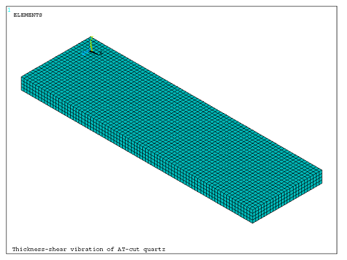
The material orientation corresponding to the AT-cut of quartz is achieved by specifying the element coordinate system (ESYS attribute for SOLID226) based on a local coordinate system (LOCAL) rotated by a -35.25 degree angle about axis X.
The electrodes are considered infinitesimally thin and are modeled by coupling VOLT degrees-of-freedom on the major surfaces of the plate. The driving AC voltage is applied to the master node of one of the coupled sets, while the other electrode is grounded.
A time harmonic analysis is performed in the 0.1 MHz vicinity of the thickness-shear mode resonance which, for an infinitely long and wide plate, is at fr = 1.666 MHz.
Structural and electric losses are introduced in the analysis by specifying the anisotropic viscosity matrix (TB,AVIS) and the dielectric loss tangent coefficients (TB,DLST).
The following material properties for quartz are used:
Table 2.15: Material Constants of α-Quartz [a]
| Elastic Stiffness: cE (109 Pa) | Phonon Viscosity, η (10-3 Pa·s) | ||
|---|---|---|---|
| c11 | 86.74 | η11 | 1.37 |
| c12 | 6.99 | η12 | 0.73 |
| c13 | 11.91 | η13 | 0.72 |
| c14 | -17.91 | η14 | 0.01 |
| c33 | 107.2 | η33 | 0.97 |
| c44 | 57.94 | η44 | 0.36 |
| c66 | 39.88 | η66 | 0.32 |
| Piezoelectric Constants: e (C/m2) | |||
| e11 | 0.171 | ||
| e14 | -0.0406 | ||
| Dielectric Permittivity: εS (10-12 F/m) | Dielectric Loss Tangent: tanδ (10-4) [b] | ||
| ε11 | 39.21 | tanδ11 | 1.6 |
| ε33 | 41.03 | tanδ33 | 1.8 |
| Mass Density: ρ (kg/m3) | |||
| ρ | 2649 | ||
The geometric properties are:
| Length (l) = 20 mm |
| Width (w) = 6 mm |
| Thickness (t) = 1 mm |
The loading for this problem is:
| Voltage (V) = 1 V |
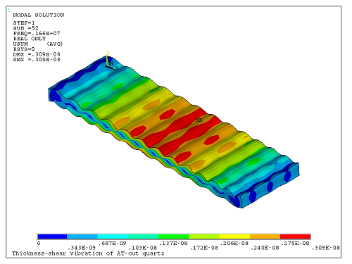
For an AT-cut quartz plate of given dimensions, the resonance and antiresonance frequencies of the thickness-shear mode (shown in the figure below) are determined to be fr = 1.664 MHz and fa = 1.668 MHz, respectively.
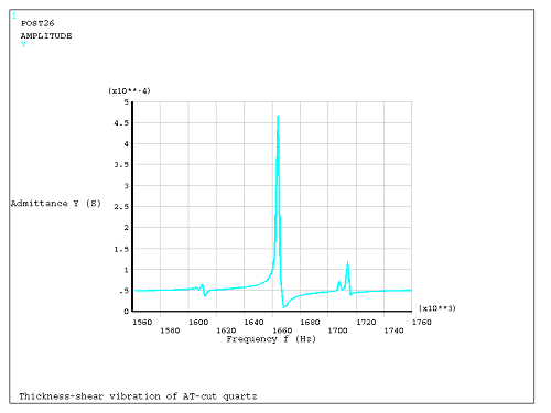
The plate admittance Y is calculated from the reaction charge Q at the master node of the loading electrode as Y = 2πfQ/V and is shown in the figure below:
The harmonic analysis results are post-processed at the resonance and antiresonance frequencies to calculate the quality factor Q and the electromechanical coupling coefficient k using the element energy records (NMISC records 1, 2, and 3), as shown in Equation 10–81 and Equation 10–83 of the Mechanical APDL Theory Reference. The results are summarized here:
Table 2.16: Thickness-Shear Vibration of AT-cut of Quartz Characteristics
| Frequency (Hz) | Quality factor (Q) | Electromechanical Coupling Coefficient (k) | |
|---|---|---|---|
| Resonance | 1.664e6 | 2217812 | 0.0261 |
| Antiresonance | 1.668e6 | 1000999 | 0.0819 |
The command listing below demonstrates the problem input. An alternative element type and alternative material input are included in the comment lines.
/title, Thickness-shear vibration of AT-cut quartz
/nopr
!! Material constants for Quartz
! - Stiffness coefficients, N/m**2
c11= 86.74e9   $ c12= 6.99e9    $ c13= 11.91e9   $  c14= -17.91e9
c33= 107.2e9
c44= 57.94e9
c66= 39.88e9

! - Viscosity coefficients, N/m**2 s
eta11= 1.37e-3 $ eta12= 0.73e-3 $ eta13= 0.72e-3 $ eta14= 0.01e-3
eta33= 0.97e-3
eta44= 0.36e-3
eta66= 0.32e-3

! - Piezoelectric stress constants, C/m**2
e11= 0.171
e14=-0.0406

! - Permittivity constants at constant strain, F/m
ep11=39.21e-12
ep33=41.03e-12

! - Dielectric loss tangent
tand11=1.6e-4
tand33=1.8e-4

! - Density, kg/m**3
rho = 2649

! - Material matrices [c],[e],[PER] in IEEE format
!
!   [c11  c12 c13  c14   0  0 ]   [ e11  0  0]   [ep11  0    0  ]
!   [c12  c11 c13 -c14   0  0 ]   [-e11  0  0]   [  0  ep11  0  ]
!   [c13  c13 c33   0    0  0 ]   [  0   0  0]   [  0   0   ep33]
!   [c14 -c14  0   c44   0  0 ]   [ e14  0  0]
!   [ 0    0   0    0  c44 c14]   [  0 -e14 0]
!   [ 0    0   0    0  c14 c66]   [  0 -e11 0]
!
! - Material matrices [c],[e],[PER] in Ansys format
!
!   [c11  c12 c13   0  c14  0 ]   [ e11  0  0]    [ep11  0    0  ]
!   [c12  c11 c13   0 -c14  0 ]   [-e11  0  0]    [  0  ep11  0  ]
!   [c13  c13 c33   0   0   0 ]   [  0   0  0]    [  0   0   ep33]
!   [ 0    0   0   c66  0  c14]   [  0 -e11 0]
!   [c14 -c14  0    0  c44  0 ]   [ e14  0  0]
!   [ 0    0   0   c14  0  c44]   [  0 -e14 0]

!  Plate dimensions
l=2e-2                    ! m
w=0.6e-2
t=0.1e-2

!  Voltage load
V=1                       ! V

/PREP7
tb,ANEL,1,,,0             ! Anisotropic elasticity table
tbda,1,c11,c12,c13,,c14
tbda,7,c11,c13,,-c14
tbda,12,c33
tbda,16,c66,,c14
tbda,19,c44
tbda,21,c44

tb,AVIS,1,,,0             ! Anisotropic viscosity table
tbda,1,eta11,eta12,eta13,,eta14
tbda,7,eta11,eta13,,-eta14
tbda,12,eta33
tbda,16,eta66,,eta14
tbda,19,eta44
tbda,21,eta44

tb,PIEZ,1,,,0             ! Piezoelectric coefficient table
tbda,1,e11
tbda,4,-e11
tbda,7
tbda,10,,-e11
tbda,13,e14
tbda,16,,-e14

eps0=8.854e-12
emunit,epzro,eps0
tb,DPER,1,,,0             ! Permittivity table
tbda,1,ep11/eps0,ep11/eps0,ep33/eps0

tb,DLST,1,,,0             ! Dielectric loss tangent
tbda,1,tand11,tand11,tand33

mp,DENS,1,rho             ! Density

local,11

!  Element coordinate system for AT-cut rotation
local,12,,,,,,-35.25

block,0,l,0,t,0,w
et,1,226,1001             ! Piezoelectric analysis option
esize,t/4
csys,11
mat,1  $ type,1 $ esys,12
vmesh,1

! Mechanical boundary conditions
nsel,s,loc,x,0
nsel,r,loc,y,0
nsel,r,loc,z,0
d,all,ux,0,,,,uy,uz
nsel,all

! Electrodes
nsel,s,loc,y,0
cp,1,volt,all
ng=ndnext(0)
nsel,s,loc,y,t
cp,2,volt,all
nd=ndnext(0)
nsel,all

d,ng,volt,0

eplot
fini

f1=1.56e6
f2=1.76e6
nsbs=100

/solve
antype,harmonic
harfrq,f1,f2
nsub,nsbs

outres,all,all
kbc,1
d,nd,volt,V
solve
fini

! Plot admittance vs. frequency
/post26
rfor,2,nd,chrg,,charge
PI2=3.14159*2.
prod,3,2,1,,Y,,,PI2/V
prvar,3
/axlab,x,Frequency f (Hz)
/axlab,y,Admittance Y (S)
plcplx,0
plvar,3
prcplx,1
prvar,3
fini

fr=1.664e6                     ! Resonance frequency
fa=1.668e6                     ! Antiresonance frequency

! Calculate coupling factor estimate
k=sqrt((fa**2-fr**2)/fa**2)
/com,
/com, *** Estimated coupling coefficient k = %k%
/com,

! Post-process resonance frequency
/post1
set,,,,0,fr
plnsol,u,sum                   ! Plot thickness-shear mode shape

! Calculate energies
etab,Ue_e,nmisc,1              ! Store element elastic energy
etab,Ud_e,nmisc,2              ! Store element dielectric energy
etab,Um_e,nmisc,3              ! Store element mutual energy
ssum                           ! Sum element energies
*get,Ue,ssum,,item,Ue_e
*get,Ud,ssum,,item,Ud_e
*get,Um,ssum,,item,Um_e

! Calculate coupling coefficient
k=abs(Um)/sqrt(Ue*Ud)

/com,
/com, *** Coupling coefficient k = %k% at resonance
/com,

! Calculate losses
set,,,,1,fr
etab,Ue_e,nmisc,1              ! Store element elastic loss
etab,Ud_e,nmisc,2              ! Store element dielectric loss
ssum                           ! Sum element losses
*get,UeIm,ssum,,item,Ue_e
*get,UdIm,ssum,,item,Ud_e

! Calculate quality factor Q
Q=(Ue+Ud)/(UeIm+UdIm)

/com,
/com, *** Quality factor Q = %Q% at resonance
/com,

! Post-process antresonance frequency
/post1
set,,,,0,fa

! Calculate energies
etab,Ue_e,nmisc,1              ! Store element elastic energy
etab,Ud_e,nmisc,2              ! Store element dielectric energy
etab,Um_e,nmisc,3              ! Store element mutual energy
ssum                           ! Sum element energies
*get,Ue,ssum,,item,Ue_e
*get,Ud,ssum,,item,Ud_e
*get,Um,ssum,,item,Um_e

! Calculate coupling coefficient
k=abs(Um)/sqrt(Ue*Ud)

/com,
/com, *** Coupling coefficient k = %k% at antiresonance
/com,

! Calculate losses
set,,,,1,fa
etab,Ue_e,nmisc,1              ! Store element elastic loss
etab,Ud_e,nmisc,2              ! Store element dielectric loss
ssum                           ! Sum element losses
*get,UeIm,ssum,,item,Ue_e
*get,UdIm,ssum,,item,Ud_e

! Calculate quality factor Q
Q=(Ue+Ud)/(UeIm+UdIm)

/com,
/com, *** Quality factor Q = %Q% at antiresonance
/com,
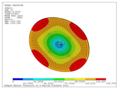
This example demonstrates a damped piezoelectric modal analysis of a barium titanate disc with dielectric losses.
The following topics are available:
A single-crystal barium titanate (BT) disc of radius A and thickness D is covered with electrodes of radius E on both surfaces. The disc is discretized using the piezoelectric option (KEYOPT(1) = 1001) of element SOLID226:
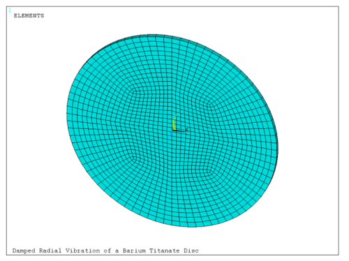
The bottom surface of the disc is simply supported (UZ = 0 at Z = 0) and the bottom electrode is grounded (VOLT degree of freedom set to 0).
A modal analysis is performed for the first six modes to identify the radial mode and calculate its characteristics. To include electric losses (dielectric loss tangent) in the simulation, the UNSYM modal solver (MODOPT,UNSYM) is chosen. Element results are turned on (MXPAND,,,,YES) to allow the calculation of energies. Two electrical configurations are explored – closed circuit (top electrode VOLT degree of freedom set to zero) and open circuit (top electrode VOLT degree of freedom is unconstrained). The first configuration corresponds to the piezoelectric resonance, and the second one to the piezoelectric antiresonance.
The following material properties for single-crystal barium titanate are used:
Table 2.17: Material Constants of Barium Titanate
| Elastic Compliance, sE (10-12 m2/N) [a] | |
|---|---|
| s11 | 8.05 |
| s33 | 15.7 |
| s12 | -2.35 |
| s13 | -5.24 |
| s44 | 18.4 |
| s66 | 8.84 |
| Piezoelectric Strain Constants, d (10-12 C/N) [a] | |
| d15 | 392 |
| d31 | -34.5 |
| d33 | 85.6 |
| Dielectric Permittivity at Constant Stress, εT/ε0 [a] | |
| ε11 /ε0 | 2920 |
| ε33 /ε0 | 168 |
| Dielectric Loss Tangent, tanδ [b] | |
| tanδ11 | 0.005 |
| tanδ33 | 0.009 |
| Density, ρ (kg/m3)[a] | |
| ρ | 6020 |
[a] Berlincourt D., Jaffe H. (1958) Elastic and piezoelectric coefficients of single-crystal barium titanate. Phys. Rev., vol 111. pp. 143-148
[b] Rehrig P. W., Trolier-McKinstry S., Park S.-E., and Messing G.L. (2000) Dielectric and Electromechanical Properties of Barium Titanate Single Crystal Grown by Templated Grain Growth. IEEE Trans. Ultrason., Ferroelectr., Freq. Control, vol. 47, no. 4, pp. 895-902
The geometric properties are:
| Disc radius (A) = 5 mm |
| Electrode radius (E) = 4.5 mm |
| Thickness (D) = 0.2 mm |
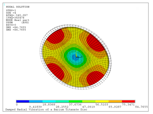
The fourth eigensolution was identified as a radial mode after visual inspection of the mode shapes (PLDISP,1) following the resonance modal analysis. The disc deformations corresponding to the resonance and antiresonance frequencies are shown in the following figures.
The modal analysis results are further post-processed to calculate two important characteristics of the piezoelectric vibrations – the quality factor Q and the electromechanical coefficient k. These parameters, along with the effective dielectric loss tangent, are summarized here for the resonance and the antiresonance of the radial mode:
Table 2.18: Radial Vibration Parameters
| Parameter | Resonance | Antiresonance |
|---|---|---|
| Damped frequency, Hz | 312820.9 | 343478.2 |
| Stability, Hz | -4.7 | -242 |
| Quality factor (Q) | 33296.5 | 709.4 |
| Electromechanical coupling coefficient (k) | 0.0634 | 0.433 |
| Effective dielectric loss tangent (tand) | 0.00746 | 0.00895 |
The quality factor Q is calculated first using the real and imaginary part of the eigenfrequency (see Equation 10–82 in the Theory Reference) and then using the real (stored energy) and imaginary (loss) parts of the element elastic (NMISC,1) and dielectric (NMISC,3) energy records (see Equation 10–81 in the Theory Reference). It is demonstrated that both methods produce the same value of Q.
The electromechanical coupling coefficient k is calculated using the element
elastic (NMISC,1), dielectric (NMISC,2), and mutual (NMISC,3) energy records
(see Equation
10–83 in the Theory Reference). The calculated value of k for
the antiresonance frequency closely agrees with the electromechanical coupling
factor estimate using the resonance and antiresonance frequencies
 = 0.413.
The effective dielectric loss tangent tand is calculated as a ratio of imaginary (loss) and real (stored energy) element dielectric energy record (NMISC,2).
The command listing below demonstrates the problem input. An alternative element type and alternative material input are included in the comment lines.
/title, Damped Radial Vibration of a Barium Titanate Disc

/com,  Problem parameters:
A=5.e-3                        ! disc radius, m
E=4.5e-3                       ! electrode radius, m
D=0.2e-3                       ! thickness, m

/com, Compliance coefficients, m^2/N
s11=8.05e-12
s12=-2.35e-12
s13=-5.24e-12
s33=15.7e-12
s44=18.4e-12
s66=8.84e-12

/com, Piezoelectric strain coefficients, C/N
d15=392e-12
d31=-34.5e-12
d33=85.6e-12

/com, Electric permittivity, relative
epT11=2920
epT33=168

eps0=8.854e-12                 ! free space permittivity, F/m

! Loss tangent coefficients
tand11=0.005                   ! radial
tand33=0.009                   ! axial

! density
rho=6020

/nopr
/PREP7
et,1,SOLID226,1001
emunit,epzro,eps0              ! Free-space permittivity

tb,dper,1,,,,1
tbdata,1,epT11,epT11,epT33

! Dielectric loss tangent table
tb,dlst,1
tbda,1,tand11,tand11,tand33

tb,anel,1,,,1                 ! Anisotropic elastic compliance matrix
tbda,1,s11,s12,s13
tbda,7,s11,s13
tbda,12,s33
tbda,16,s66
tbda,19,s44
tbda,21,s44

tb,piez,1,,,1                 ! Piezoelectric strain matrix
tbda,1,,,d31
tbda,4,,,d31
tbda,7,,,d33
tbda,13,,d15
tbda,16,d15

tblist,all,all

mp,dens,1,rho

cyl4,,,0,0,E,90,D
cyl4,,,0,90,E,180,D
cyl4,,,0,180,E,270,D
cyl4,,,0,270,E,360,D

cyl4,,,e,0,A,90,D
cyl4,,,e,90,A,180,D
cyl4,,,e,180,A,270,D
cyl4,,,e,270,A,360,D

vglue,all
esize,2*D
vmesh,all
finish

/prep7
nsel,s,loc,x,0
d,all,ux
nsel,s,loc,y,0
d,all,uy

nsel,s,loc,z
d,all,uz
nsel,all

! Boundary conditions and loads
csys,1                         ! cylindrical CS
nsel,s,loc,z,0
nsel,r,loc,x,0,E
cp,1,volt,all                  ! define bottom electrode
*get,n_grd,node,0,num,min      ! get master node on bottom electrode
nsel,s,loc,z,D
nsel,r,loc,x,0,E
cp,2,volt,all                  ! top electrode
*get,n_load,node,0,num,min     ! get master node on top electrode
nsel,all
csys,0

d,n_grd,volt,0                 ! ground bottom electrode
fini

! Damped modal analysis (Resonance)
/solu
antyp,modal
nmodes=6
modopt,unsym,nmodes
mxpand,nmodes,,,yes            ! calculate element results
d,n_load,volt,0                ! resonance electric BC
solve
*get,f4r_Re,mode,4,stab        ! resonance, real part
*get,f4r_Im,mode,4,dfrq        ! resonance, imag part
fini

! Post-process damped modal analysis results (Resonance)
/post1
*do,i,1,nmodes
set,1,i
pldisp,1
!/wait,3
*enddo

! Radial mode
set,1,4                        ! real solution for mode 4
plnsol,u,sum                   ! plot displacement

! Quality factor via complex eigenfrequencies
Q1=f4r_Im/(2*abs(f4r_Re))


! Calculate energies
etab,Ue_e,nmisc,1              ! store element elastic energy
etab,Ud_e,nmisc,2              ! store element dielectric energy
etab,Um_e,nmisc,3              ! store element mutual energy
ssum                           ! sum element energies
*get,Ue,ssum,,item,Ue_e
*get,Ud,ssum,,item,Ud_e
*get,Um,ssum,,item,Um_e

! Calculate coupling coefficient
k=abs(Um)/sqrt(Ue*Ud)

! Calculate losses
set,1,4,,1                     ! imaginary solution for mode 4
etab,Ue_e,nmisc,1              ! store element elastic loss
etab,Ud_e,nmisc,2              ! store element dielectric loss
ssum                           ! sum element losses
*get,UeIm,ssum,,item,Ue_e
*get,UdIm,ssum,,item,Ud_e

! Calculate effective dielectric loss tangent
tand=UdIm/Ud

! Calculate quality factor via energies
Q2=(Ue+Ud)/(UeIm+UdIm)

/com,
/com, *** Resonance:
/com,     - damped frequency dfrq = %f4r_Im% Hz
/com,     - stability stab = %f4r_Re% Hz
/com,     - Q-factor (eigenfrequencies) Q1 = %Q1%
/com,     - Q-factor (energy) Q2 = %Q2%
/com,     - Electromechanical coupling (energy) k =%k%
/com,     - Effective dielectric loss tangent tand = %tand%
/com,
fini

! Damped modal analysis (Antiresonance)
/solu
antyp,modal
nmodes=6
modopt,unsym,nmodes
mxpand,nmodes,,,yes            ! calculate element results

ddele,n_load,volt              ! antiresonance electric BC
solve
*get,f4a_Re,mode,4,stab        ! antiresonance, real part
*get,f4a_Im,mode,4,dfrq        ! antiresonance, imag part
fini

! Post-process damped modal analysis results (Antiresonance)
/post1
! Radial mode
set,1,4
plnsol,u,sum                   ! plot displacement

! Quality factor via complex eigenfrequencies
Q1=f4a_Im/(2*abs(f4a_Re))

! Calculate energies
etab,Ue_e,nmisc,1              ! store element elastic energy
etab,Ud_e,nmisc,2              ! store element dielectric energy
etab,Um_e,nmisc,3              ! store element mutual energy
ssum                           ! sum element energies
*get,Ue,ssum,,item,Ue_e
*get,Ud,ssum,,item,Ud_e
*get,Um,ssum,,item,Um_e

! Coupling coefficient
k=abs(Um)/sqrt(Ue*Ud)

! Calculate losses
set,1,4,,1                     ! imaginary solution for mode 4
etab,Ue_e,nmisc,1              ! store element elastic loss
etab,Ud_e,nmisc,2              ! store element dielectric loss
ssum                           ! sum element losses
*get,UeIm,ssum,,item,Ue_e
*get,UdIm,ssum,,item,Ud_e

! Effective dielectric loss tangent
tand=UdIm/Ud

! Quality factor via energies
Q2=(Ue+Ud)/(UeIm+UdIm)

/com,
/com, *** Antiresonance:
/com,     - damped frequency dfrq = %f4a_Im% Hz
/com,     - stability stab = %f4a_Re% Hz
/com,     - Q-factor (eigenfrequencies) Q1 = %Q1%
/com,     - Q-factor (energy) Q2 = %Q2%
/com,     - Electromechanical coupling (energy) k =%k%
/com,     - Effective dielectric loss tangent tand = %tand%
/com,
fini

! Coupling coefficient via eigenfrequencies
fr=f4r_Im
fa=f4a_Im
k=sqrt((fa**2-fr**2)/fa**2)
/com,
/com,     - Electromechanical coupling (eigenfrequencies) k =%k%
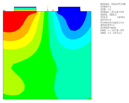
This example models two electrodes on a piezoelectric substrate surrounded by piezoelectric perfectly matched layers. A harmonic analysis is performed.
The following topics are available:
In this example, an acoustic wave is exited in the piezoelectric substrate by applying electric potentials of magnitude 1 V and 0 V, respectively, to the metallic electrodes shown in the figure:
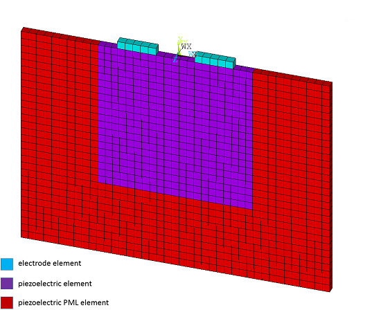
The piezoelectric substrate is surrounded by a piezoelectric perfectly matched layer (PML) to reduce the wave reflection from the boundary.
The electrodes are modeled using the SOLID186 structural element type. Both piezoelectric domains—the substrate and the PML—are modeled using the piezoelectric analysis option (KEYOPT(1) = 1001) of SOLID226. In addition, KEYOPT(15) is set to 1 for the piezoelectric PML layer. PMLOPT command defines the normal reflection coefficients.
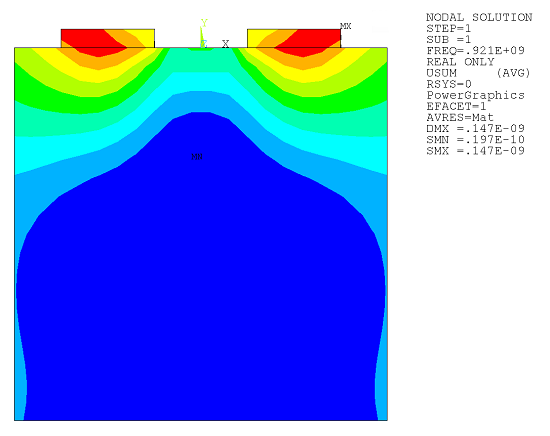
A harmonic analysis is performed at 921 MHz to determine the displacement and potential distributions in the piezoelectric substrate.
The material properties for the electrode are:
| Elastic modulus = 70×109 N/m2 |
| Poisson’s ratio = 0.35 |
| Density = 2700 kg/m3 |
The material properties for the piezoelectric substrate are:
| Density = 7489 kg/m3 |
| Relative permittivities: (ep11) = 402.078, (ep22) = 402.078, (ep33) = 329.794 |
| Piezoelectric stress coefficients: (e13) = -4.1 C/m2, (e23) = -4.1 C/m2, (e33) = 14.1 C/m2, (e52) = 10.5 C/m2, (e61) = 10.5 C/m2 |
| Piezoelectric anisotropic elastic coefficients: (d11) = 13.2×10¹⁰ N/m2, (d21) = 7.1×10¹⁰ N/m2, (d22) = 13.2×10¹⁰ N/m2, (d31) = 7.3×10¹⁰ N/m2, (d32) = 7.3×10¹⁰ N/m2, (d33) = 11.5×10¹⁰ N/m2, (d44) = 3.0×10¹⁰ N/m2, (d55) = 2.6×10¹⁰ N/m2, (d66) = 2.6×10¹⁰ N/m2 |
The geometric properties are:
| Electrode width = 1 µm |
| Electrode height = 0.2 µm |
| Piezoelectric substrate thickness = 4 µm |
| Piezoelectric PML layer thickness = 2 µm |
| Model depth = 0.2 µm |
The loading for this problem is:
| Electrode voltage = 1 V |
The nodal displacement and voltage amplitude solutions under the operating frequency are shown below.
/title, Piezoelectric Perfectly Matched Layers

/nopr
pi=acos(-1)

prd=4                ! Electrode period (um)
w_elctrd=1           ! Electrode width (um)
t_elctrd=0.2         ! Electrode height (um)
n_elctrd=2           ! Number of electrodes (um)

t_sbstrt=4           ! Substrate thickness (um)
d_PML=2              ! PML thickness (um)
d=t_elctrd           ! Model depth
esz=prd/20           ! Element size (um)

E_elctrd=70e9        ! Electrode elastic modulus (N/m^2)
nu_elctrd=0.35       ! Electrode Poisson's ratio
dnsty_elctrd=2700    ! Electrode density (kg/m^3)

frqncy=0.921e9       ! Operating frequency

rho = 7489           ! Piezoelectric substrate density (kg/m^3)

! Permittivities
ep11 = 402.078
ep22 = 402.078
ep33 = 329.794

! Piezoelectric matrix values (C/m^2)
e11 = 0         $e12 = 0         $e13 = -4.1
e21 = 0         $e22 = 0         $e23 = -4.1
e31 = 0         $e32 = 0         $e33 = 14.1
e41 = 0         $e42 = 0         $e43 = 0
e51 = 0         $e52 = 10.5      $e53 = 0
e61 = 10.5      $e62 = 0         $e63 = 0

! Elastic matrix values (N/m^2)
$d11=13.2e10
$d21=7.1e10 $d22=13.2e10
$d31=7.3e10 $d32=7.3e10 $d33=11.5e10
$d41=0      $d42=0      $d43=0      $d44=3.0e10
$d51=0      $d52=0      $d53=0      $d54=0      $d55=2.6e10
$d61=0      $d62=0      $d63=0      $d64=0      $d65=0      $d66=2.6e10

/prep7

! Geometry

wpcsys,-1,0
wpoffs,-prd/4
block,-w_elctrd/2,w_elctrd/2,,t_elctrd,,d
vgen,2,all,,,prd/2

wpcsys,-1,0
block,-prd/2,prd/2,,-t_sbstrt,,d
vglue,all
vsel,s,loc,y,0,t_elctrd
vatt,1,1,1

vsel,inve
vatt,2,2,2,11
allsel
cm,keep_v,volu

vsel,none
block,-(prd/2+d_PML),(prd/2+d_PML),,-t_sbstrt-d_PML,,d
cm,scrap_v,volu

alls
cmsel,all
vsbv,scrap_v,keep_v,,dele,keep
cmsel,u,keep_v
vatt,3,3,3,11
allsel
vplot

wpcsys,-1,0         ! Local coordinate system 11 (z aligned with global x)
wprota,,,90
cswpla,11
csys

! Electrode

et,1,SOLID186            ! 3D structural solid element type
mp,ex,1,E_elctrd
mp,nuxy,1,nu_elctrd
mp,dens,1,dnsty_elctrd

! Piezoelectric substrate

et,2,SOLID226,1001       ! 3D piezoelectric element type
mp,perx,2,ep11
mp,pery,2,ep22
mp,perz,2,ep33

tb,piez,2,,18
tbdata,1,e11,e12,e13,e21,e22,e23
tbdata,7,e31,e32,e33,e41,e42,e43
tbdata,13,e51,e52,e53,e61,e62,e63

tb,anel,2,,21,0
tbdata,1,d11,d21,d31,d41,d51,d61
tbdata,7,d22,d32,d42,d52,d62,d33
tbdata,13,d43,d53,d63,d44,d54,d64
tbdata,19,d55,d65,d66

mp,dens,2,rho

! Piezoelectric PML

et,3,SOLID226,1001   ! 3D piezoelectric element type
keyopt,3,15,1        ! PML option for SOLID226
psys                 ! PML element coordinate system defaults to global Cartesian
mp,perx,3,ep11
mp,pery,3,ep22
mp,perz,3,ep33

tb,piez,3,,18
tbdata,1,e11,e12,e13,e21,e22,e23
tbdata,7,e31,e32,e33,e41,e42,e43
tbdata,13,e51,e52,e53,e61,e62,e63

tb,anel,3,,21,0
tbdata,1,d11,d21,d31,d41,d51,d61
tbdata,7,d22,d32,d42,d52,d62,d33
tbdata,13,d43,d53,d63,d44,d54,d64
tbdata,19,d55,d65,d66

mp,dens,3,rho

! Meshing

esize,esz
vsel,s,mat,,1,2
vsweep,all
vsel,s,mat,,3
psys,0
vsweep,all

! Electrode voltage excitation

vsel,s,mat,,1
nslv,s,1
nsel,r,loc,x,0,prd
vsel,s,mat,,2
nslv,r,1
d,all,volt,0       ! Ground electrode
allsel

vsel,s,mat,,1
nslv,s,1
nsel,r,loc,x,0,-prd
vsel,s,mat,,2
nslv,r,1
d,all,volt,1       ! Voltage load
allsel

vlscale,all,,,1e-6,1e-6,1e-6,,,1
finish

! Harmonic analysis

/solu
pmlopt,,,1.e-4,1.e-4,1.e-4,1.e-4,1.e-4,1.e-4,yes  ! Set piezoelectric PML normal reflection coefficient
antype,harm
harfrq,frqncy
solve
finish

! Postprocessing

/post1
set,1,1,,ampl
esel,s,type,,2
nsle,s,all
nsel,r,loc,x,0,-1/2
nsel,r,loc,y,0
nsel,r,loc,z,0
prnsol,u
prnsol,volt
allsel
esel,s,type,,1
esel,a,type,,2
plnsol,u,sum
plnsol,volt
finish
Other piezoelectric analysis examples are found in the Mechanical APDL Verification Manual:
See also these more comprehensive examples in the Technology Showcase: Example Problems: