


A thermal-electric analysis can account for the following thermoelectric effects:
Joule heating - Heating occurs in a conductor carrying an electric current. Joule heat is proportional to the square of the current, and is independent of the current direction.
Seebeck effect - A voltage (Seebeck EMF) is produced in a thermoelectric material by a temperature difference. The induced voltage is proportional to the temperature difference. The proportionality coefficient is know as the Seebeck coefficient (α).
Peltier effect - Cooling or heating occurs at the junction of two dissimilar thermoelectric materials when an electric current flows through the junction. Peltier heat is proportional to the current, and changes sign if the current direction is reversed.
Thomson effect - Heat is absorbed or released in a non-uniformly heated thermoelectric material when electric current flows through it. Thomson heat is proportional to the current, and changes sign if the current direction is reversed.
Typical applications include heating coils, fuses, thermocouples, and thermoelectric coolers and generators. For more information, refer to Thermoelectrics.
The following related topics are available:
- 2.2.1. Elements Used in a Thermal-Electric Analysis
- 2.2.2. Performing a Thermal-Electric Analysis
- 2.2.3. Example: Thermoelectric Cooler Analysis
- 2.2.4. Example: Thermoelectric Generator Analysis
- 2.2.5. Example: Transient Thermoelectric Analysis of a Peltier Cooler
- 2.2.6. Other Thermal-Electric Analysis Examples
Several elements are available for modeling thermal-electric coupling. Table 2.3: Elements Used in Thermal-Electric Analyses summarizes them briefly. For detailed descriptions of the elements and their characteristics (degrees of freedom, KEYOPT options, inputs and outputs, etc.), see the Element Reference.
LINK68 and SHELL157 are special purpose thermal-electric elements. The coupled-field elements (SOLID5, SOLID98, PLANE222, PLANE223, SOLID225, SOLID226, SOLID227, and LINK228 ) require you to select the element degrees of freedom for a thermal-electric analysis: TEMP and VOLT. For SOLID5 and SOLID98, set KEYOPT(1) to 0 or 1. For PLANE222, PLANE223, SOLID225, SOLID226, SOLID227, and LINK228, set KEYOPT(1) to 110.
Table 2.3: Elements Used in Thermal-Electric Analyses
| Elements | Thermoelectric Effects | Material Properties | Analysis Types |
|---|---|---|---|
|
LINK68 - Thermal-Electric Line SOLID5 - Coupled-Field Hexahedral SOLID98 - Coupled-Field Tetrahedral SHELL157 - Thermal-Electric Shell | Joule Heating |
KXX, KYY, KZZ RSVX, RSVY, RSVZ DENS, C, ENTH |
Static Transient (transient thermal effects only) |
|
PLANE222 - Coupled-Field Quadrilateral PLANE223 - Coupled-Field Quadrilateral SOLID225 - Coupled-Field Hexahedral SOLID226 - Coupled-Field Hexahedral SOLID227 - Coupled-Field Tetrahedral LINK228 - Coupled-Field Line |
Joule Heating Seebeck Effect Peltier Effect Thomson Effect |
KXX, KYY, KZZ RSVX, RSVY, RSVZ DENS, C, ENTH SBKX SBKY, SBKZ PERX, PERY, PERZ |
Static Transient (transient thermal and electrical effects) |
The analysis can be either steady-state (ANTYPE,STATIC) or transient (ANTYPE,TRANS). It follows the same procedure as a steady-state or transient thermal analysis. (See Steady-State Thermal Analysis and Transient Thermal Analysis.)
To perform a thermal-electric analysis, you need to specify the element type and material properties. For Joule heating effects, you must define both electrical resistivity (RSVX, RSVY, RSVZ) and thermal conductivity (KXX, KYY, KZZ). Mass density (DENS), specific heat (C), and enthalpy (ENTH) may be defined to take into account thermal transient effects. These properties may be constant or temperature-dependent.
A transient analysis using PLANE222, PLANE223, SOLID225, SOLID226, SOLID227, or LINK228 can account for both transient thermal and transient electrical effects. You must define electric permittivity (PERX, PERY, PERZ) to model the transient electrical effects. A transient analysis using LINK68, SOLID5, SOLID98, or SHELL157 can only account for transient thermal effects.
To include the Seebeck-Peltier thermoelectric effects, you need to specify a PLANE222, PLANE223, SOLID225, SOLID226, SOLID227, or LINK228 element type and a Seebeck coefficient (SBKX, SBKY, SBKZ) (MP). You also need to specify the temperature offset from zero to absolute zero (TOFFST). To capture the Thomson effect, you need to specify the temperature dependence of the Seebeck coefficient (MPDATA).
Be sure to define all data in consistent units. For example, if the current and voltage are specified in amperes and volts, you must use units of watts/length-degree for thermal conductivity. The output Joule heat will then be in watts.
For problems with convergence difficulties, activate the line-search capability (LNSRCH).
This example problem considers the performance of a thermoelectric cooler described in Direct Energy Conversion (Third Edition) by Stanley W. Angrist, Ch. 4, p.161 (1976).
The following related topics are available:
A thermoelectric cooler consists of two semiconductor elements connected by a copper strap. One element is an n-type material and the other is a p-type material. The n-type and p-type elements have a length L, and a cross-sectional areas A = W2, where W is the element width. The cooler is designed to maintain the cold junction at temperature Tc, and to dissipate heat from the hot junction Th on the passage of an electric current of magnitude I. The positive direction of the current is from the n-type material to the p-type material as shown in the following figure.

The dimensions of the copper strap were chosen arbitrarily. See the command input listing for the dimensions used. The effect on the results is negligible.
The semiconductor elements have the following dimensions:
| Length L = 1 cm |
| Width W = 1 cm |
| Cross-sectional area A = 1 cm2 |
The thermoelectric cooler has the following material properties.
Table 2.4: Material Properties
| Component | Resistivity (ohm*cm) | Thermal Conductivity (watt/cm°C) | Seebeck Coefficient (μvolts/°C) |
|---|---|---|---|
| n-type material | ρn = 1.05 x 10⁻³ | λn = .013 | α n = -165 |
| p-type material | ρp = 0.98 x 10⁻³ | λp = .012 | α p = 210 |
| Connecting straps (copper) | 1.7 x 10⁻⁶ | 400 | — |
First Thermal-Electric Analysis
A 3D steady-state thermal-electric analysis is carried out to evaluate the performance of the cooler. The givens are: Tc = 0°C, Th = 54°C, and I = 28.7 amps. The following quantities are calculated and compared to analytical values.
The heat rate Qc that must be pumped away from the cold junction to maintain the junction at Tc:
Qc = αTcI - 1/2 I2R - KΔT
where: Combined Seebeck coefficient α = |α n| + |α p| Internal electrical resistance R = (ρn+ ρp)L/A Internal thermal conductance K = (λn + λp)A/L Applied temperature difference ΔT = Th - Tc The power input:
P = VI = αI(ΔT) + I2R
where: V = voltage drop across the cooler The coefficient of performance:
β = Qc/P
Second Thermal-Electric Analysis
The inverse problem is solved. The givens are: Qc = 0.74 watts, Th = 54°C, and I = 28.7 amps and the cold junction temperature Tc and the temperature distribution are determined.
The first thermal-electric analysis is performed by imposing a temperature constraint Tc = 0 ºC on the cold junction and an electric current I on the input electric terminal. The rate of heat removed from the cold junction Qc is determined as a reaction solution at the master node. The input power P is determined from the voltage and current at the input terminal. The coefficient of performance is calculated from Qc and P. Numerical results are compared in Table 2.5: Thermoelectric Cooler Results to the analytical design from the reference. A small discrepancy between the numerical and analytical results is due to the presence of the connecting straps.
Table 2.5: Thermoelectric Cooler Results
| Quantity | Results | Reference Results |
|---|---|---|
| Qc, watts | 0.728 | 0.74 |
| P, watts | 2.292 | 2.35 |
| β | 0.317 | 0.32 |
In the second analysis, an inverse problem is solved: Qc from the first solution is imposed as a rate of heat flow on the cold junction to determine the temperature at that junction. The calculated temperature of the cold junction Tc = 0.106 ºC is close to the expected 0 ºC. The following figure shows the temperature distribution.
/title, Thermoelectric Cooler
/com
/com  Reference: "Direct Energy Conversion" (third edition) by
/com              Stanley W. Angrist
/com              Ch.4 "Thermoelectric Generators", p. 164
/com
/VUP,1,z
/VIEW,1,1,1,1
/TRIAD,OFF
/NUMBER,1
/PNUM,MAT,1
/nopr

/PREP7
! cooler dimensions
l=1e-2               ! element length, m
w=1e-2	             ! element width, m
hs=0.1e-2            ! strap height, m

toffst,273           ! Temperature offset, deg.C

! n-type material
mp,rsvx,1,1.05e-5    ! Electrical resistivity, Ohm*m
mp,kxx,1,1.3         ! Thermal conductivity, watt/(m*K)
mp,sbkx,1,-165e-6    ! Seebeck coefficient, volt/K

! p-type material
mp,rsvx,2,0.98e-5    ! Electrical resistivity, Ohm*m
mp,kxx,2,1.2         ! Thermal conductivity, watt/(m*K)
mp,sbkx,2,210e-6     ! Seebeck coefficient,volt/K

! Connecting straps (copper)
mp,rsvx,3,1.7e-8     ! Resistivity, Ohm*m
mp,kxx,3,400         ! Thermal conductivity, watt/(m*K)

! FE model
et,1,226,110         ! 20-node thermo-electric brick
block,w/2,3*w/2,,w,,l
block,-3*w/2,-w/2,,w,,l
block,-3*w/2,3*w/2,,w,l,l+hs
block,-1.7*w,-w/2,,w,-hs,0
block,w/2,1.7*w,,w,-hs,0
vglue,all

esize,w/3
type,1
mat,1
vmesh,1
mat,2
vmesh,2
msha,1,3d
mat,3
lesize,61,hs
lesize,69,hs
lesize,30,w/4
lesize,51,w/4
lesize,29,w/4
lesize,50,w/4
vmesh,6,8

eplot

! Boundary conditions and loads
nsel,s,loc,z,l+hs    ! Cold junction
cp,1,temp,all        ! Couple TEMP dofs
nc=ndnext(0)         ! Get master node number

nsel,s,loc,z,-hs     ! Hot junction
d,all,temp,54        ! Hold at Th, deg. C

nsel,s,loc,x,-1.7*w  ! First electric terminal
d,all,volt,0         ! Ground

nsel,s,loc,x,1.7*w   ! Second electric terminal
cp,2,volt,all        ! Couple VOLT dofs
ni=ndnext(0)         ! Get master node
nsel,all
fini

/SOLU                ! First solution
antype,static
d,nc,temp,0          ! Hold cold junction at Tc, deg.C
I=28.7
f,ni,amps,I          ! Apply current I, Amps to the master node
solve
fini

/com
*get,Qc,node,nc,rf,heat  ! Get heat reaction at cold junction
/com
/com Heat absorbed at the cold junction Qc = %Qc%, watts
/com
P=volt(ni)*I
/com Power input P = %P%, watts
/com
/com Coefficient of performance beta = %Qc/P%
/com

/SOLU                ! Second solution
ddele,nc,temp        ! Delete TEMP dof constraint at cold junction
f,nc,heat,Qc         ! Apply heat flow rate Qc to the cold junction
solve
fini

/com
/com Temperature at the cold junction Tc = %temp(nc)%, deg.C
/com

/SHOW,WIN32c         ! Use /SHOW,X11C for X Window System
/CONT,1,18           ! Set the number of contour plots
/POST1
plnsol,temp          ! Plot temperature distribution
fini
This example problem considers the performance of a power producing thermoelectric generator described in Direct Energy Conversion (Third Edition) by Stanley W. Angrist, Ch. 4, p.156 (1976).
A thermoelectric generator consists of two semiconductor elements. One element is an n-type material and the other is a p-type material. The n-type and p-type elements have lengths Ln and Lp, and cross-sectional areas An = Wnt and Ap = Wpt, where Wn and Wp are the element widths and t is the element thickness. The generator operates between temperature Tc (a cold junction) and temperature Th (a hot junction). The hot sides of the elements are coupled in temperature and voltage. The cold sides of the elements are connected to an external resistance Ro. The temperature difference between the cold and hot sides generates electric current I and power Po in the load resistance.

The semiconductor elements have the following dimensions.
Table 2.6: Semiconductor Element Dimensions
| Dimension | n-type Material | p-type Material |
|---|---|---|
| Length L | 1 cm | 1 cm |
| Width W | 1 cm | 1.24 cm |
| Thickness t | 1 cm | 1 cm |
The operating conditions are:
| Cold junction temperature Tc = 27°C |
| Hot junction temperature Th = 327°C |
| External resistance Ro = 3.92 x 10⁻³ ohms |
Two 3D steady-state thermal-electric analyses are performed to evaluate the thermal efficiency of the generator.
First Thermal-Electric Analysis
A thermal-electric analysis is performed using the following material properties at the average temperature of 177°C (Angrist, Ch.4, p.157).
Table 2.7: Material Properties
| Component | Resistivity (ohm*cm) | Thermal Conductivity (watt/cm°C) | Seebeck Coefficient (μvolts/°C) |
|---|---|---|---|
| n-type material | ρn = 1.35 x 10⁻³ | λn = .014 | α n = -195 |
| p-type material | ρp = 1.75 x 10⁻³ | λp = .012 | α p = 230 |
The following quantities are calculated and compared to the analytical values:
The thermal input to the hot junction:
Qh = αThI - 1/2 I2R + KΔT
where: Combined Seebeck coefficient α = |α n| + |α p| Internal electrical resistance R = ρn(Ln/ An) + ρp(Lp/ Ap) Internal thermal conductance K = λn(An/Ln) + λp(Ap/Lp) Applied temperature difference ΔT = Th - Tc The electric current:
I = αΔT/(R + Ro)
The output power:
Po = I2Ro
The thermal efficiency:
η = Po/Qh
Second Thermal-Electric Analysis
This is the same as the first analysis, except that the temperature dependence of the Seebeck coefficient, electrical resistivity, and thermal conductivity of the materials is taken into account using the following data (Angrist, Appendix C, p.476–477).
The following table shows the results using material properties at the average temperature of 177°C.
Table 2.8: Results Using Material Properties at Average Temperature
| Quantity | Results | Reference Results |
|---|---|---|
| Qh, watts | 13.03 | 13.04 |
| I, amps | 19.08 | 19.2 |
| Po, watts | 1.43 | 1.44 |
| η, % | 10.96 | 10.95 |
The following table shows the results when temperature dependence of the material properties is taken into account.
Table 2.9: Results Considering Material Temperature Dependence
| Quantity | Results |
|---|---|
| Qh, watts | 11.07 |
| I, amps | 16.37 |
| Po, watts | 1.05 |
| η, % | 9.49 |
/title, Thermoelectric Generator
/com
/com  Reference: "Direct Energy Conversion" (3rd edition) by
/com              Stanley W. Angrist
/com              Ch.4 "Thermoelectric Generators", p. 156
/com
/com
! Generator dimensions
ln=1.e-2                 ! n-type element length, m
lp=1.e-2                 ! p-type element length, m
wn=1.e-2                 ! n-type element width, m
wp=1.24e-2               ! p-type element width, m
t=1.e-2                  ! element thickness, m
d=0.4e-2                 ! Distance between the elements

rsvn=1.35e-5             ! Electrical resistivity, Ohm*m
rsvp=1.75e-5
kn=1.4                   ! Thermal conductivity, watt/(m*K)
kp=1.2
sbkn=-195e-6             ! Seebeck coeff, volt/deg, n-type
sbkp=230e-6              !                          p-type
Th=327                   ! Temperature of hot junction, deg.C
Tc=27                    ! Temperature of cold side, deg.C
Toffst=273               ! Temperature offset, deg.C
R0=3.92e-3               ! External resistance, Ohm

/nopr
/PREP7
et,1,SOLID226,110        ! 20-node thermoelectric brick
/com
/com *** Thermo-electric analysis with material
/com *** properties evaluated at an average temperature
/com
! Material properties for n-type material
mp,rsvx,1,rsvn
mp,kxx,1,kn
mp,sbkx,1,sbkn

! Material properties for p-type material
mp,rsvx,2,rsvp
mp,kxx,2,kp
mp,sbkx,2,sbkp

! Solid model
block,d/2,wn+d/2,-ln,0,,t
block,-(wp+d/2),-d/2,-lp,0,,t

! Meshing
esize,wn/2
mat,1
vmesh,1
mat,2
vmesh,2

toffst,Toffst            ! Temperature offset

! Boundary conditions and loads
nsel,s,loc,y,0           ! Hot side
cp,1,temp,all            ! couple TEMP dofs
nh=ndnext(0)             ! Get master node
d,nh,temp,Th             ! Set TEMP constraint to Th
cp,2,volt,all            ! couple VOLT dofs
nsel,all

nsel,s,loc,y,-ln         ! Cold side, n-type
nsel,r,loc,x,d/2,wn+d/2
d,all,temp,Tc
cp,3,volt,all            ! Input electric terminal
nn=ndnext(0)             ! Get master node
nsel,all

nsel,s,loc,y,-lp         ! Cold side, p-type
nsel,r,loc,x,-(wp+d/2),-d/2
d,all,temp,Tc            ! Set TEMP constraint to Tc
cp,4,volt,all            ! Output electric terminal
np=ndnext(0)             ! Get master node
nsel,all
d,np,volt,0              ! Ground

et,2,CIRCU124,0          ! Load resistor
r,1,R0
type,2
real,1
e,np,nn
fini

/SOLU
antype,static
cnvtol,heat,1,1.e-3      ! Set convergence values
cnvtol,amps,1,1.e-3      ! for heat flow and current
solve
fini

/post1
set,last

! n-branch area
An=wn*t
! p-branch area
Ap=wp*t
! Total thermal conductance
K=kp*Ap/lp+kn*An/ln
! Total electric resistance of the couple
R=lp*rsvp/Ap+ln*rsvn/An
! Combined Seebeck coefficient
alp=abs(sbkp)+abs(sbkn)
/com
/com   ***   Calculated and expected results:
/com
/com Heat pumping rate on cold side Qh, watts
*get,Qh,node,nh,rf,heat
/com  - ANSYS: %Qh%
I_a=alp*(Th-Tc)/(R+R0)
Qh_a=alp*I_a*(Th+Toffst)-I_a**2*R/2+K*(Th-Tc)
/com  - Expected: %Qh_a%
/com
/com Electric current I drawn from the generator, Amps
*get,I,elem,21,smisc,2
/com - ANSYS: %I%
/com - Expected: %I_a%
/com
/com Output power P, watts
*get,P0,elem,21,nmisc,1
/com - ANSYS: %P0%
P0_a=I**2*R0
/com - Expected: %P0_a%
/com
/com Coefficient of thermal efficiency
/com - ANSYS: %P0/Qh%
/com - Expected: %P0_a/Qh_a%
/com ---------------------------------------------------
/com
/com *** Thermo-electric analysis with temperature
/com *** dependent material properties
/com

/PREP7
! Temperature data points
mptemp,1,25,50,75,100,125,150
mptemp,7,175,200,225,250,275,300
mptemp,13,325,350

! n-type material
! Seebeck coefficient, Volt/K
mpdata,sbkx,1,1,-160e-6,-168e-6,-174e-6,-180e-6,-184e-6,-187e-6
mpdata,sbkx,1,7,-189e-6,-190e-6,-189e-6,-186.5e-6,-183e-6,-177e-6
mpdata,sbkx,1,13,-169e-6,-160e-6

mpplot,sbkx,1

! Electrical resistivity, Ohm*m
mpdata,rsvx,1,1,1.03e-5,1.06e-5,1.1e-5,1.15e-5,1.2e-5,1.28e-5
mpdata,rsvx,1,7,1.37e-5,1.49e-5,1.59e-5,1.67e-5,1.74e-5,1.78e-5
mpdata,rsvx,1,13,1.8e-5,1.78e-5

mpplot,rsvx,1

! Thermal conductivity, watts/(m*K)
mpdata,kxx,1,1,1.183,1.22,1.245,1.265,1.265,1.25
mpdata,kxx,1,7,1.22,1.19,1.16,1.14,1.115,1.09
mpdata,kxx,1,13,1.06,1.03

mpplot,kxx,1

! p-type material
! Seebeck coefficient, Volt/K
mpdata,sbkx,2,1,200e-6,202e-6,208e-6,214e-6,220e-6,223e-6
mpdata,sbkx,2,7,218e-6,200e-6,180e-6,156e-6,140e-6,120e-6
mpdata,sbkx,2,13,101e-6,90e-6

mpplot,sbkx,2

! Electrical resistivity, Ohm*m
mpdata,rsvx,2,1,1.0e-5,1.08e-5,1.18e-5,1.35e-5,1.51e-5,1.7e-5
mpdata,rsvx,2,7,1.85e-5,1.98e-5,2.07e-5,2.143e-5,2.15e-5,2.1e-5
mpdata,rsvx,2,13,2.05e-5,2.0e-5

mpplot,rsvx,2

! Thermal conductivity, watts/(m*K)
mpdata,kxx,2,1,1.08,1.135,1.2,1.25,1.257,1.22
mpdata,kxx,2,7,1.116,1.135,1.13,1.09,1.12,1.25
mpdata,kxx,2,13,1.5,2.025

mpplot,kxx,2

/SOLU
tunif,Tc
neqit,30
solve
fini

/post1
set,last

/com
/com   ***   Results
/com
*get,Qh,node,nh,rf,heat
/com Heat pumping rate on cold side Qh = %Qh%, watts
/com
*get,I,elem,21,smisc,2
/com Electric current drawn from the generator I = %I%, Amps
/com
*get,P,elem,21,nmisc,1
/com Output power P = %P%, watts
/com
/com Coefficient of thermal efficiency beta = %P/Qh%
/com ---------------------------------------------------
This example problem considers the transient response of a Peltier cooler subject to a current pulse as described in G.J. Snyder, J.-P. Fleurial, T. Caillat, R. Yang, and G. Chen, "Supercooling of Peltier cooler using a current pulse," J. Appl. Phys., v.92, n.3, pp.1564-1569 (2002).
The Peltier cooler consists of two thermoelectric elements – n-type Bi2Te3 and p-type Bi2Te3 – soldered to a copper foil on top. The thermoelectric elements have the following dimensions:
| Height H = 5.8 mm |
| Cross-sectional area A = 1 mm2 |
| Distance between the elements D = 1.4 mm. |
The copper foil is 35 µm thick. The lateral dimensions of the foil were chosen arbitrarily. See the command input listing for the dimensions used.
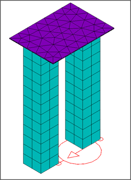
The thermoelectic elements and the copper foil are modeled using the thermal-electric analysis option (KEYOPT(1) = 110) of hexahedral- and tetrahedral-shaped SOLID225, respectively, as shown in Figure 2.6: Finite Element Model .
A transient analysis is performed to demonstrate the supercooling of the cold junction (top side) due to the application of a square current pulse to the hot (bottom) side of the device. The temperature of the hot side remains fixed at -14 °C during the simulation.
The electric pulse is applied using the current source option (KEYOPT(1)=3) of CIRCU124 element and is characterized by the following parameters:
| Steady-state current Is = 0.675 Amps |
| Pulse amplitude Ip = 2.5 Is |
| Pulse duration = 4 s. |
The following material properties were used in the simulation.
Table 2.10: Material Properties
| Component | Resistivity (ohm*m) | Thermal Conductivity (Watt/mK) | Specific Heat (J/kgK) | Density (kg/m3) | Seebeck Coefficient (Volt/K) |
| n-type Bi2Te3 | 0.9x10⁻⁵ | 1.6 | 154.4 | 7740 | -181x10-6 [a] |
| p-type Bi2Te3 | 0.9x10⁻⁵ | 1.6 | 154.4 | 7740 | 181x10-6 [a] |
| Copper | 1.7x10⁻⁸ | 350 | 385 | 8920 | 6.5x10⁻⁶ |
[a] Seebeck coefficients were adjusted to match the temperature difference between the cold and hot sides at steady state.
The current load was applied in four intervals over a total period of 26 s. The electric pulse used to achieve the supercooling is shown in Figure 2.7: Applied Current Pulse along with the respective temperature of the cold junction in Figure 2.8: Cold Junction Temperature. The cold side temperature evolution with time is in good agreement with the experimental results reported by Snyder et al.

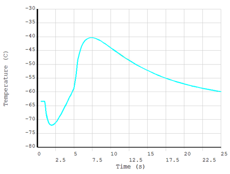
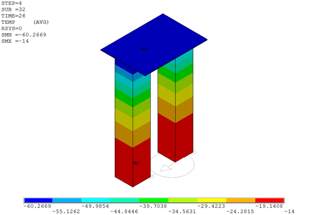
Figure 2.9: Temperature Distribution shows the temperature distribution in the cooler at the end of the simulation.
Following is the problem input. All text prefaced with an exclamation point (!) is a comment.
/title, Supercooling of Peltier cooler using a current pulse
/com
/com Reference:
/com  G.J.Snyder, J.-P.Fleurial, T.Caillat, R.Yang, G.Chen (2002)
/com  "Supercooling of Peltier cooler using a current pulse,"
/com  in J.Appl.Phys., v.92, n.3, pp.1564-1569
/com
/com Experimental curve (Fig. 2 shifted by 1 sec):
/com  T=-63 C @ t=1 s   (steady-state)
/com  T=-72 C @ t=2 s   (Minimum temperature)
/com  T=-71 C @ t=3 s   (returning to steady-state after supercooling)
/com  T=-68 C @ t=4 s   (returning to steady-state after supercooling)
/com  T=-63 C @ t=5 s   (returning to steady-state after supercooling)
/com  T=-52 C @ t=6 s   (heating-up)
/com  T=-43 C @ t=7 s   (heating-up)
/com  T=-41 C @ t=8 s   (heating-up)
/com  T=-41C @ t=9 s    (heating-up)
/com  T=-42 C @ t=10 s  (heating-up)
/com  T=-43 C @ t=11 s  (heating-up)
/com  T=-44.5 C @ t=12 s (returning to steady-state)
/com  T=-45.5 C @ t=13 s (returning to steady-state)
/com  T=-46.5 C @ t=14 s (returning to steady-state)
/com  T=-48 C @ t=15 s  (returning to steady-state)
/com  T=-49 C @ t=16 s  (returning to steady-state)
/com  T=-50 C @ t=17 s  (returning to steady-state)
/com  T=-51 C @ t=18 s  (returning to steady-state)
/com  T=-52 C @ t=19 s  (returning to steady-state)
/com  T=-53 C @ t=20 s  (returning to steady-state)
/com  T=-53.5 C @ t=21 s (returning to steady-state)
/com  T=-54 C @ t=22 s  (returning to steady-state)
/com  T=-55 C @ t=23 s  (returning to steady-state)
/com  T=-56 C @ t=26 s  (returning to steady-state)
/com
/VUP,1,z
/VIEW,1,1,1,1

/PREP7
a=1e-3	         ! thermoelement width, m
h=5.8e-3             ! thermoelement height, m
d=1.4e-3             ! distance between the elements,m

ls=3.5e-3            ! copper connector length, m
ws=2.5e-3            ! copper connector width, m
hs=0.035e-3          ! copper connector height, m

tunif,20             ! Ambient temperature, deg.C
toffst,273           ! Temperature offset, deg.C

! n-type Bi2Te3
mp,rsvx,1,0.9e-5     ! Electrical resistivity, Ohm*m
mp,kxx,1,1.6         ! Thermal conductivity, watt/(m*K)
mp,sbkx,1,-181e-6    ! Seebeck coeff, volt/K
mp,c,1,154.4         ! Heat capacity, J/kg*K
mp,dens,1,7740       ! Density, kg/m^3

! p-type Bi2Te3
mp,rsvx,2,0.9e-5     ! Electrical resistivity, Ohm*m
mp,kxx,2,1.6         ! Thermal conductivity, watt/(m*K)
mp,sbkx,2,181e-6     ! Seebeck coeff, volt/K
mp,c,2,154.4         ! Heat capacity, J/kg*K
mp,dens,2,7740       ! Density, kg/m^3

! Copper sheet
mp,rsvx,3,1.7e-8     ! Electrical resistivity, Ohm*m
mp,kxx,3,350         ! Thermal conductivity, Watt/(m*K)
mp,sbkx,3,6.5e-6     ! Seebeck coefficient, volt/K
mp,c,3,385           ! Heat capacity, J/kg*K
mp,dens,3,8920       ! Density, kg/m^3

! FE model
et,1,225,110         ! 8-node thermo-electric brick
et,2,225,110         ! tet-degenerated 8-node thermo-electric brick

block,d/2,a+d/2,-a/2,a/2,,h
block,-(a+d/2),-d/2,-a/2,a/2,,h
block,-ls/2,ls/2,-ws/2,ws/2,h,h+hs
vglue,all

type,1
esize,a/2
mat,1
vmesh,1
mat,2
vmesh,2

type,2
mat,3
msha,1,3d
lesize,33,hs
lesize,25,a/3
lesize,27,a/3
vmesh,4

nsel,s,loc,z,h+hs    ! Cold side
cp,1,temp,all
nc=ndnext(0)

nsel,s,loc,z,0       ! Hot side
d,all,temp,-14       ! deg. C

nsel,s,loc,z,0       ! First electric terminal
nsel,r,loc,x,-(a+d/2),-d/2
cp,2,volt,all
ng=ndnext(0)
d,ng,volt,0

nsel,s,loc,z,0       ! Second electric terminal
nsel,r,loc,x,d/2,a+d/2
cp,3,volt,all
ni=ndnext(0)
nsel,all

Is=0.675             ! Steady-state electric current, Amps
Ip=2.5*Is            ! Current pulse, Amps
et,3,124,3           ! Current source
r,1,Is
type,3
real,1
e,ng,ni
fini

/SOLU
antype,trans
outres,all,all
kbc,1
deltim,0.5
time,1
timint,off
solve

deltim,0.1
time,5
r,1,Ip
timint,on
solve

deltim,0.25
time,10
r,1,Is
solve

deltime,0.5
time,26
solve
fini

/post26
esel,s,ename,,Circu124
e124=elnext(0)
esel,all
esol,2,e124,,smisc,2
/xrange,0,25
/yrange,0,2
/axlab,x, Time (s)
/axlab,y, Current (Amps)
plvar,2

nsol,3,nc,temp
prvar,3
/xrange,0,25
/yrange,-80,-30
/axlab,x, Time (s)
/axlab,y,Temperature (C)
plvar,3
fini
Other thermal-electric analysis examples are found in the Mechanical APDL Verification Manual: