For all calculations when using a pressure-based segregated solver (SIMPLE, SIMPLEC, or PISO) or for steady-state calculations when using the pressure-based coupled solver or the density-based implicit solver, you have the option of solving your flow with a pseudo time method. The pseudo time method is a form of implicit under-relaxation, described in Pseudo Time Method Under-Relaxation in the Theory Guide.
To apply pseudo time method under-relaxation, perform the following:
Select the Density-Based solver or the Pressure-Based solver. Except when you are using a pressure-based segregated solver, you must also select Steady for the time dependence.
 Setup →
  General
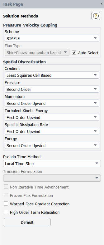
Go to the Solution Methods task page (Figure 36.30: The Solution Methods Task Page).
Solution → MethodsIf you are using the pressure-based solver, the Coupled scheme under Pressure-Velocity Coupling is the default. You can also select one of the other segregated schemes (SIMPLE, SIMPLEC, or PISO).
If you are using the density-based solver, select the Implicit scheme under Formulation.
Select one of the following from the Pseudo Time Method drop-down list:
The Local Time Step method is available for a pressure-based segregated solver. Complete the setup for this method, as described in Local Time Step Method Setting.
The Global Time Step method is available for the pressure-based coupled solver or the density-based implicit solver. Complete the setup for this method, as described in Global Time Step Method Settings.
Note:
The Global Time Step method is selected by default when using the pressure-based coupled solver for single-phase flows that do not include the battery, fuel cell, and/or solidification and melting models.
When using a pressure-based segregated solver, the Local Time Step method is not available with the following:
the structural model
multiphase models
the G Equation model (as part of the premixed or partially premixed combustion model)
the crevice model
Non-Iterative Time Advancement (NITA)
When using a pressure-based segregated solver, the Local Time Step method is not supported with the species transport model when the energy equation is disabled.
When Local Time Step is selected from the Pseudo Time Method list (for a case with the pressure-based segregated solver), the local pseudo time step size for each cell in the domain is based on your specified Pseudo Time Courant Number (see Local Time Step Method in the Theory Guide), which is available in the Solution Controls Task Page (Figure 36.31: The Solution Controls Task Page for the Local Time Step Method). You can also set the under-relaxation factor for each equation in the field next to its name under Pseudo Time Under-Relaxation Factors.
![]() Solution →
Solution → ![]() Controls
Controls
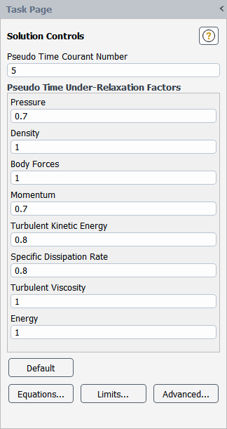
Note that the Local Time Step method is recommended for better convergence behavior. While using a smaller value for the Pseudo Time Courant Number can improve the convergence behavior, it can also slow down the convergence rate.
When Global Time Step is selected from the Pseudo Time Method list (for a steady-state case with the pressure-based coupled solver or density-based implicit solver), pseudo time method under-relaxation is applied. You can also specify an explicit under-relaxation of the equation to control the update of computed variables at each iteration (see Pseudo Time Method Under-Relaxation in the Theory Guide). The default values of under-relaxation parameters for all variables are set to values that work well for most of the cases. It is good practice to start a calculation with the default under-relaxation parameters. If your case exhibits divergence or the residuals continue to increase after a few iterations, then you should reduce the under-relaxation factors.
To have further control over the parameters for each individual equation, you can specify advanced solution controls. Note that all equations can be modified, except for flow equations (that is, pressure and momentum). Generally, you will not need to enter equation-specific solution parameters. However, it may help in cases where a particular equation is giving convergence problems.
Finally, you must define settings for the running of the calculation: the pseudo time step size or time scale factor for the fluid and solid zones.
For details on defining these global time step method settings, see the following sections:
When Global Time Step is selected from the Pseudo Time Method list in the Solution Methods task page, you can modify the pseudo time explicit relaxation factors in the Solution Controls Task Page (Figure 36.32: The Solution Controls Task Page for the Global Time Step Method).
![]() Solution →
Solution → ![]() Controls
Controls
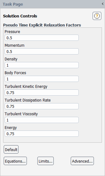
You can set the under-relaxation factor for each equation in the field next to its name under Pseudo Time Explicit Relaxation Factors.
Important: If you are using the pressure-based coupled solver, all equations will have an associated under-relaxation factor (see Under-Relaxation of Equations in the Theory Guide). If you are using the density-based implicit solver, only those equations that are solved sequentially (see Density-Based Solver in the Theory Guide) will have under-relaxation factors.
If you change under-relaxation factors, but you then want to return to Ansys Fluent’s default settings, you can click the button.
When Global Time Step is selected from the Pseudo Time Method list in the Solution Methods task page, Ansys Fluent provides two options to improve convergence in the Expert tab of in the Advanced Solution Controls dialog box (Figure 36.33: The Advanced Solution Controls Dialog Box for the Pseudo Time Method):
Specify a time scale factor for the equation-specific time step size in lieu of using a uniform global pseudo time step size. This scaling factor scales the pseudo time step size employed for the flow equations specified in the Run Calculation task page (see Pseudo Time Settings for the Calculation).
Use the standard steady-state method by turning off the pseudo time method usage for that particular equation. Here, the corresponding under-relaxation factor to be employed with that equation may be specified. The default values of under-relaxation parameters for all variables are set to values that work well for most of the cases.
The default setting will have the pseudo time method usage turned on for all equations with the corresponding time scale factor set to unity, except when one of the combustion models is used. When a pseudo time method is selected in combustion cases, the species, enthalpy, and combustion variable equations will only use the pseudo time method if it is manually enabled in the Expert tab. Also, when using the premixed or partially-premixed combustion models, the pseudo time method can be manually enabled for the energy variable in the Expert tab.
By default, all user-defined scalars (UDS) have the pseudo time method usage disabled. This is because the physical parameters of the UDS and the appropriate time scale are not known to the solver before starting the calculation. You can manually enable the pseudo time method usage for UDS under the Expert tab in the Advanced Solution Controls Dialog Box.
![]() Solution → Controls
Solution → Controls ![]() Advanced...
Advanced...
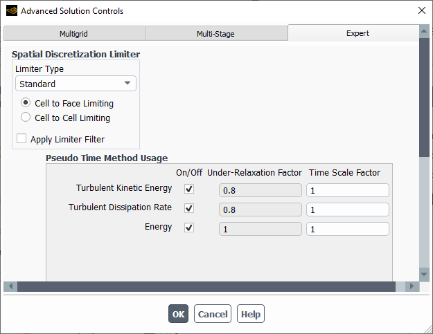
Specify the equation-specific steady-state solution method for a particular equation (if needed) by enabling or disabling the pseudo time method usage using the On/Off check box next to the equation. The dialog box then allows either specification of a pseudo Time Scale Factor or Under-Relaxation Factor for that particular equation based on the check box setting.
Note: For multiphase flows, the pseudo time method expert options for the volume fraction equation are available only when it is solved in a segregated fashion. It is not available when the Coupled with Volume Fractions option is enabled in the Solution Methods task page (see Selecting the Pressure-Velocity Coupling Method for information about this setting).
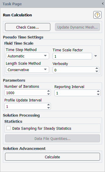
When Global Time Step is selected from the Pseudo Time Method list in the Solution Methods task page, you can specify the time step size for the Fluid Zone and/or the Solid Zone under Pseudo Time Settings in the Run Calculation task page (Figure 36.34: The Run Calculation Task Page for the User-Specified Pseudo Time Step Method).
![]() Solution →
Solution → ![]() Run Calculation
Run Calculation
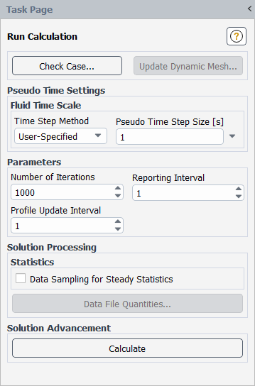
Select the Time Step Method for the Fluid Time Scale.
If you choose User-Specified, you will enter the Pseudo Time Step Size, which is used for every equation unless the equation specific time step is used for a particular equation, as mentioned in Advanced Solution Controls for the Pseudo Time Method. Typically, the time scale size should be relevant to the global time scale of the flow, for example:
where
 is a representative length scale for the geometry (such as chord length).
If you use the default Automatic method (see Figure 36.35: The Run Calculation Task Page for the Automatic Pseudo Time Step Method), the pseudo time step size is calculated internally and used for each equation listed, unless the equation has a time step size specified as noted in Advanced Solution Controls for the Pseudo Time Method. The automatic time scale is calculated from time scales estimated for various physics active in the simulation. For more information, refer to Global Time Step Method in the Theory Guide.
You can control the convergence process by adjusting the automatic pseudo time step size value using the Time Scale Factor field, which simply scales the calculated time step size by the specified value. The automatic time scale calculation is often somewhat conservative, and increasing the Time Scale Factor to
3or10can often increase the convergence rate. Less commonly, you may need to reduce its value to0.3or0.1for better convergence.Alternatively, you can also fine-tune the automatic pseudo time step size by choosing the Length Scale Method used to calculate its value. The following options are available in the drop-down list:
Conservative : (default) uses the cube root of the mesh volume for 3D cases and square root of area for 2D cases.
Aggressive : uses the maximum geometry extent, leading to a larger time step size than Conservative.
User-Specified allows you to directly control the Length Scale. This method is particularly useful in problems that have a specific length scale that is difficult to determine from the overall geometry of the problem. For example, in the case of flow over an airfoil, the appropriate length scale would be the length of the airfoil instead of the length scale calculated based on the geometry of the entire domain.
You can specify the Verbosity. This is an integer value of 0, 1, or 2. The default value is 0. A value of 1 prints the pseudo time step size. A value of 2 prints additional details about the calculation.
Select the Time Step Method for the Solid Time Scale.
Note: The Solid Time Scale group box is only available when the Energy equation is enabled with a solid zone in the domain, the Porous Zone option enabled, or the Solidification & Melting model enabled.
If you choose User-Specified, you will enter the Pseudo Time Step Size, which is used where the Solid Time Scale is needed (that is, solid zones, porous zones, and/or solidification/melting model).
If you choose Automatic, which is the default method, the pseudo time step size is calculated internally as described in Global Time Step Method in the Theory Guide. Specify a Time Scale Factor to control/adjust the pseudo time step size obtained from the automatically calculated Solid Time Scale.
Continue setting up your solution as you would a steady-state run, as described in Performing Steady-State Calculations.