Band-pass filtering of a complex transient solution provides for the separate analysis of different time scales in a broadband spectrum. This postprocessing method is implemented in Ansys Fluent by means of the inverse DFT, which can be performed for any Runtime DFT dataset of either the frequency band or single tone type, see Runtime Discrete Fourier Transformation in the Fluent User's Guide. This is useful in the postprocessing of scale-resolving simulations of turbulent flows, especially when the aeroacoustics phenomena are analyzed. The inverse DFT procedure is built into the solution animation workflow of Ansys Fluent, where it can replace the transient solution calculation through its transient reconstruction using the known spectrum within a desired band or for a selected single tone.
The following limitations apply to the inverse DFT tool:
Animations can only be generated for single graphical objects of either a Contour or XY Plot.
Scene animations are not supported.
With beta features enabled (as described in Introduction), you can create an inverse DFT animation after the accumulation of
the corresponding Runtime DFT dataset is completed. This is indicated by a
0 in the Samples to Complete read-only field
on the Zone-Specific Sampling Options dialog box, see Zone-Specific Sampling Options Dialog Box for Runtime DFT - Frequency
Band in the Fluent User's Guide.
To set up a contour plot or an XY plot to be animated using Inverse DFT:
Select in the contour or XY plot, the field variable for the desired DFT dataset in the Inverse DFT… category.
This category contains a field variable for each DFT dataset as soon as this dataset is created. Note that the inverse DFT field variable for a dataset remains zero until the beginning of the inverse DFT reconstruction process. You can estimate the fixed range of values for your animation (the color range for a contour plot or the axis range for an XY plot) using the corresponding DFT magnitude variable.
After the graphical object is created, set up a solution animation for this graphical object in the standard way by selecting the Animation Definition tool either in the Ribbon or Outline View.
 Solution → Activities → Create → Solution
Animations...
Solution → Activities → Create → Solution
Animations...See details in Animating the Solution in the Fluent User's Guide for creating an animation.
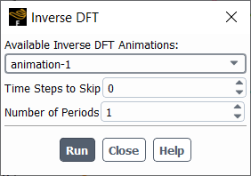
Instead of the standard animation of a transient solution, the animation frames are created during an inverse DFT reconstruction run. To perform this run, open the Figure 21.1: Inverse DFT Dialog Box:
Results → Animation → Inverse
DFT...In this dialog box, the selection list Available Inverse DFT Animations shows only those animation objects that were created using field variables from the Inverse DFT… category. The integer entry field Time Steps to Skip lets you reconstruct a frequency-filtered solution with a coarser time resolution. The integer entry field Number of Periods lets you specify the animation duration. For a frequency band, the reference period for the animation duration corresponds to the minimum frequency in a band. Click Run to start the inverse DFT computation.
The text commands, which correspond to the Inverse DFT dialog box, are located in menu
/solve/animate/inverse-dftTo playback the animation, use the standard animation tool:
Results → Animation → Solution
Playback...