


Higher turbulent gas-liquid bubbly flows are encountered in many industrial applications, including petrochemical, pharmaceutical, biochemical, nuclear, and metallurgical industries [452]. One common example of such flows is annular two-phase flow that occurs in boilers, heat exchangers, natural gas well, and so on. In the annular flow pattern, gas flows at high velocity through the core of the pipe, and the liquid film flows at lower velocity around the pipe wall. The high gas velocity results in large shear velocities, which, in turn, lead to high interfacial shear stress. The liquid film interface becomes unstable, and the droplets are torn from the interface and entrained in the gas core. Droplet entrainment changes flow characteristics. Different factors affect the entrained liquid fraction and the circumferential distribution of liquid film thickness on the wall. Gravity causes the liquid film drainage. Evaporation can also deplete the liquid wall film resulting in dry patches near the top of the pipe. These effects become more significant with increasing gas velocity and can result in equipment damage.
The traditional multiphase approaches to solving such problems do not predict the correct transitional flow behavior and mechanics behind droplet entrainment. In such regimes, the liquid droplet entrainment has a significant impact on the mechanisms for mass, momentum, and energy transfer. Hydrodynamic and surface forces can cause a significant deformation of the liquid film interface, resulting in the breakage of the continuous film surface into smaller dispersed droplets. The deformation depends on the flow pattern and the interface shape.
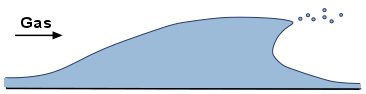
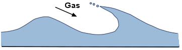
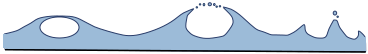
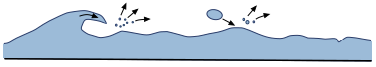
Ishii and Grolmes ([271]) identified that liquid droplets can be entrained into a gas flow in the following patterns:
Tearing off the tops of the crests of large-amplitude roll waves by the turbulent gas flow. The drag force acting on the wave top deforms the interface against the retaining force of the liquid surface tension.
Undercutting the liquid film by the gas flow. The gas penetrates the wave which starts to bulge and may eventually break.
Bursting of gas bubbles. The thinning liquid film of the bubble rising to the gas-liquid interface rupture into droplets of various sizes.
Impinging of a wave or droplet onto the film interface. A large amplitude wave may collapse into the liquid body generating droplets. Also, some droplet created by the previous mechanisms may impinge into the liquid phase producing smaller droplets.
Ansys Fluent uses the Algebraic Interfacial Area Density (AIAD) approach that offers the universal droplet entrainment model that covers all of the entrainment patterns and predicts the rate of entrainment. The AIAD approach models the momentum exchange dependent on the morphological form of the flow pattern. The model uses the volume fraction values to differentiate between bubbles, droplets, and the interface.
The AIAD framework was originally developed by Thomas Höhne from the Helmholtz-Zentrum Dresden-Rossendorf in close cooperation with Ansys ([253], [250], [254], [162], [135], [452], [455]) to overcome known limitations of the modeling of separated / stratified flows. Using the volume fraction compression scheme, which is part of the Multi-Fluid VOF model, the AIAD model supports the simulation of three phases such as continuous gas, continuous liquid, and a dispersed entrained phase (that is, droplets). Depending of the detected morphology (dispersed droplets, dispersed bubbles, or free surface), different drag and interfacial area density formulations are used. The AIAD mass transfer mechanism is used to model the breakage of the continuous liquid phase into the dispersed phase of the same material (entrainment), and inclusion of the dispersed phase into the continuous fluid phase (absorption). The entrained phase can be further extended via population balance approaches (direct quadrature method of moments (DQMOM), inhomogeneous discrete method, and so on), through which the physical distribution of the entrained phase can be obtained.
The correlations for the interfacial area density and the drag coefficient cover a full
range of phase volume fractions from gas-only to liquid-only. The AIAD approach improves the
physical modeling in the asymptotic limit between bubbly and droplet flows by using blending
functions based on volume fraction. These functions for droplets, bubbles, and free surface
morphologies ( ,
,  , and
, and  ) are defined as:
 | (14–455) |
 | (14–456) |
 | (14–457) |
where  and
and  are volume fractions of the liquid and gaseous phases, respectively,
 and
and  are the blending coefficients for droplets and bubbles, respectively,
 and
and  are the volume fraction limiters for droplets and bubbles, respectively, and
the subscripts
are the volume fraction limiters for droplets and bubbles, respectively, and
the subscripts  ,
,  , and
, and  refer to the droplets, bubbles, and free surface, respectively. The default
values are
refer to the droplets, bubbles, and free surface, respectively. The default
values are  =
=  = 50. These values are based on a number of parametric studies ([253], [250], [254]). The
default value for
= 50. These values are based on a number of parametric studies ([253], [250], [254]). The
default value for  and
and  is 0.3, which is chosen based on the approximated critical volume fraction.
The bubbles and droplets that leave the free-surface interface are initially assumed to be
spherical with constant diameters  and
and  , respectively. The interfacial area densities for these phases
  and
and  are calculated as:
 | (14–458) |
 | (14–459) |
For the free surface interphase, the interfacial area density  depends on the gradient of the liquid volume fraction
  :
:
 | (14–460) |
where  is the normal vector of the free surface.
The sum of the interfacial areas  weighted by the corresponding blending function
  gives the local interfacial area
  :
:
 | (14–461) |
Unlike one-velocity methods, such as Volume of Fluid (VOF), multi-fluid approaches consider velocity and turbulence of each phase, which induces the velocity difference between the fluids (slip velocity). The drag between the phases can be expressed using the volumetric density and the area density instead of the surface area:
 | (14–462) |
where  is the drag coefficient,
  is the slip velocity, and
  is the mixture density. If the free surface flow is considered,
the phase averaged density is used:
is the mixture density. If the free surface flow is considered,
the phase averaged density is used:
 | (14–463) |
where  and
and  are the densities of the gas and liquid phases,
respectively.
are the densities of the gas and liquid phases,
respectively.
In free surface flows, Equation 14–462 and Equation 14–463 do not represent realistic behavior of the physics at the interface. Höhne and Valle ([253]) assume that the shear stress close to the free surface acts similarly to wall shear stress on both sides of the interface to reduce the velocity differences on both phases. The free-surface interface region behaves as a wall with a wall-like shear stress that acts at the free surface, which can lead to a decrease of gas velocity. The gradients of the void fraction determine the normal vector components. The shear stress at the interface is calculated by computing the scalar product between the gradient normal to the interface and the gradients of the two fluid velocities.
The wall-like free surface shear stress vector can be calculated as a product of
the viscous stress tensor and the surface normal vector  :
:
 | (14–464) |
which translates into:
 | (14–465) |
Equation 14–465 can be rearranged as:
 | (14–466) |
 | (14–467) |
where  is the dynamic viscosity. The drag-force correlation (Equation 14–462) can be the presented as the wall shear stress force acting at the
free surface:
is the dynamic viscosity. The drag-force correlation (Equation 14–462) can be the presented as the wall shear stress force acting at the
free surface:
 | (14–468) |
The modification of the drag coefficient for the free surface can be written as:
 | (14–469) |
where  and
and  are the wall-like shear stresses.
The AIAD model also uses the definition of drag coefficients for the bubble and droplet
phases  and
and  . The default values of 0.44 for these coefficients corresponds to a typical
spherical fluid particle flow. You can define your own coefficients using user-defined functions
(UDFs).
. The default values of 0.44 for these coefficients corresponds to a typical
spherical fluid particle flow. You can define your own coefficients using user-defined functions
(UDFs).
The total drag coefficient is calculated as:
 | (14–470) |
In traditional two-phase flow problems, the small waves at the interface created by Kelvin-Helmholtz instabilities are neglected. However, although these waves are smaller than the mesh size, they may have a significant influence on the turbulence kinetic energy of the liquid phase.
Gravity and surface tension tend to stabilize the liquid surface [80]. The surface behavior depends on the following two parameters:
Turbulence Froude number: Is the ratio of fluids inertia to gravitational forces:

(14–471)
where
 is the turbulent velocity [m/s],
  is gravity [m/s2], and
  is the length scale [m].
Weber number: Is a measure of the relative importance of the fluid’s inertia compared to its surface tension:

(14–472)
where
 is the surface tension coefficient, and
 is the density of the liquid phase.
These two numbers should be considered to correctly model the behavior of the interface. The AIAD takes these numbers into account by delineating a critical region of parameter space between quiescent surfaces and surfaces that completely break up.
Based on the Froude and Weber numbers, the following regimes can be distinguished ([80], [251]):
 << 1,
<< 1,
 << 1: Weak turbulence
 The turbulence is not strong enough to cause significant surface disturbance.
 >> 1,
>> 1,
 << 1: Knobbly flow
 The turbulence is sufficient to deform the surface against gravity, but only at small length scales. Surface tension creates a very smooth and rounded interface surface.
 << 1,
<< 1,
 >> 1: Turbulence dominated by gravity
 Surface deformation is countered by gravity, resulting in a nearly flat interphase surface. The turbulent energy is high enough to disturb the surface at relatively small scales, creating small regions of waves, vortex dimples, and scars. This is the most common state in nature.
 >> 1,
>> 1,
 >> 1: Strong turbulence
 The turbulence is strong enough to counter gravity, and the surface tension is no longer sufficient to keep the flow stable.
Figure 14.11: Length-Turbulence Velocity Diagram for Water depicts the length-velocity diagram for water
[80]. It shows a prediction of the interface shape in the logarithmic
space of the length scale  and the liquid turbulence
  .
.
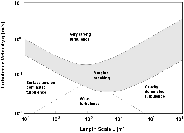
The shaded area represents the region of marginal breaking estimated by the critical Weber number and the critical Froude number. This region also shows the variations in the interface which is no longer smooth due to the turbulent flow. Because of the multi-scale nature of turbulence, these regions may occur side-by-side. The production term for the turbulent kinetic energy caused by these disturbances can be expressed as:
 | (14–473) |
The contribution to the turbulent kinetic energy produced by these unresolved waves can be calculated by the following:
 | (14–474) |
Lower and upper bounds of the region that represents the changes between an interface disturbed by turbulences and an interface that reaches a breaking point are defined as ([251]):
 | (14–475) |
 | (14–476) |
where  is a typical length scale of dominant interface features, and
 is the scalar product of interface normal and gravity
vector.
is the scalar product of interface normal and gravity
vector.
Figure 14.12: Droplet Entrainment at the Interface
shows an average location of the phase
interface.  represents a point on the average interface,
  is the inward unit normal vector, and
  is the outward component of the average liquid phase velocity.
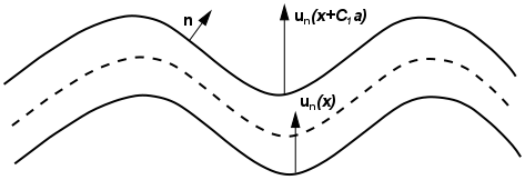
The entrainment method proposed by Höhne for the AIAD approach [252] assumes that the interface becomes destabilized due to turbulence,
forming fluid particles with an average size of  in a layer close to the interface. This layer has a thickness of
 , where
  is a non-dimensional parameter. The quantity of fluid passing the interfacial
layer relative to the velocity of the interface affects the entrained particle formation. The
entrained phase is formed from the film only if the liquid bubble moves into the gas continuous
phase relative to the interface.
is a non-dimensional parameter. The quantity of fluid passing the interfacial
layer relative to the velocity of the interface affects the entrained particle formation. The
entrained phase is formed from the film only if the liquid bubble moves into the gas continuous
phase relative to the interface.
The roughness at the interface is calculated as:
 | (14–477) |
where  is a non-dimensional parameter,
  is gravity, and
  is the local turbulent kinetic energy, which includes the subgrid
wave turbulent contribution. The AIAD approach provides a realistic modeling of the
interface between two continuous fluids by taking into account the accurate modeling
of subgrid turbulence phenomenon affecting the interface.
is the local turbulent kinetic energy, which includes the subgrid
wave turbulent contribution. The AIAD approach provides a realistic modeling of the
interface between two continuous fluids by taking into account the accurate modeling
of subgrid turbulence phenomenon affecting the interface.
A local deposition rate can be defined as:
 | (14–478) |
where  is the inward component of the average phase velocity on the interface, and
 is a user-specified constant. The parameter
  depends on the fluid properties. The default value of 0.02 has shown to work
for various applications that involve the AIAD model. The entrained phase is distributed as a
volume source at the interface in a layer with thickness
depends on the fluid properties. The default value of 0.02 has shown to work
for various applications that involve the AIAD model. The entrained phase is distributed as a
volume source at the interface in a layer with thickness  . The frequency of the entrained phase formation can be expressed as:
 | (14–479) |
The turbulent kinetic energy and the outward velocity gradient  are the key variables to calculate the deposition rate
  . The rate of entrained liquid particles (that is, droplets) from the
continuous phase is expressed as:
. The rate of entrained liquid particles (that is, droplets) from the
continuous phase is expressed as:
 | (14–480) |
where  is calculated by Equation 14–457,
  and
and  are the volume fraction and the density of the secondary continuous phase,
respectively.
are the volume fraction and the density of the secondary continuous phase,
respectively.
If the entrained phase formation occurs under the continuous fluid surface, or the entrained phase comes into contact with the continuous phase of the same material, then the entrained-phase absorption results in mass transfer of the entrained droplets to the continuous liquid phase. This can be described as:
 | (14–481) |
In Equation 14–481,  is the volume fraction of the entrained phase (droplets or bubbles),
 is the density of the entrained phase,
  is the numerical time step defined in the simulation, and
  is the blending function (the subscript
  refers to bubbles (
 ) or droplets (
 ) depending on the entrained phase).
The entrained phase formation occurs in a layer of thickness of smeared interface
 where
where  is the characteristic cell length.
Within the AIAD framework, the entrained phase complements the liquid and gas continuous phases to form a three-phase flow. The entrained phase can further grow, which can be modeled via aggregation and breakage kernels using population balance models, such as the Inhomogeneous Discrete method or Direct Quadrature Method of Moments (DQMOM) described in chapter Population Balance Model in the Ansys Fluent Theory Guide.
In Ansys Fluent, the entrainment and absorption mechanism are combined into one AIAD mass transfer mechanism. A positive mass transfer represents the entrainment of the continuous fluid into the dispersed phase, while a negative mass transfer represents the absorption of the entrained phase into the continuous fluid.
For more information on how to use the AIAD model, refer to Using the Algebraic Interfacial Area Density (AIAD) Model in the Fluent User's Guide.