


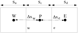
By default, Ansys Fluent stores discrete values of the scalar  at the cell centers (
 and
and  in Figure 23.3: Control Volume Used to Illustrate Discretization of a Scalar
Transport Equation). However, face values
in Figure 23.3: Control Volume Used to Illustrate Discretization of a Scalar
Transport Equation). However, face values
 are required for the convection terms in Equation 23–2 and must be interpolated from the cell center values. This is
accomplished using an upwind scheme.
are required for the convection terms in Equation 23–2 and must be interpolated from the cell center values. This is
accomplished using an upwind scheme.
Upwinding means that the face value  is derived from quantities in the cell upstream, or "upwind,"
relative to the direction of the normal velocity
is derived from quantities in the cell upstream, or "upwind,"
relative to the direction of the normal velocity  in Equation 23–2.
Ansys Fluent allows you to choose from several upwind schemes: first-order
upwind, second-order upwind, and QUICK. These schemes are described in First-Order Upwind Scheme – QUICK Scheme.
in Equation 23–2.
Ansys Fluent allows you to choose from several upwind schemes: first-order
upwind, second-order upwind, and QUICK. These schemes are described in First-Order Upwind Scheme – QUICK Scheme.
The diffusion terms in Equation 23–2 are central-differenced and are always second-order accurate.
For information on how to use the various spatial discretization schemes, see Choosing the Spatial Discretization Scheme in the User’s Guide.
When first-order accuracy is desired, quantities at cell faces are determined by assuming
that the cell-center values of any field variable represent a cell-average value and hold
throughout the entire cell; the face quantities are identical to the cell quantities. Thus when
first-order upwinding is selected, the face value  is set equal to the cell-center value of
  in the upstream cell.
Important: First-order upwind is available in the pressure-based and density-based solvers.
When second-order accuracy is desired, quantities at cell faces are computed using a
multidimensional linear reconstruction approach [44]. In this
approach, higher-order accuracy is achieved at cell faces through a Taylor series expansion of
the cell-centered solution about the cell centroid. Thus when second-order upwinding is
selected, the face value  is computed using the following expression:
 | (23–4) |
where  and
and  are the cell-centered value and its gradient in the upstream cell, and
 is the displacement vector from the upstream cell centroid to the face
centroid. This formulation requires the determination of the gradient
is the displacement vector from the upstream cell centroid to the face
centroid. This formulation requires the determination of the gradient  in each cell, as discussed in Evaluation of Gradients and Derivatives.
Finally, the gradient
in each cell, as discussed in Evaluation of Gradients and Derivatives.
Finally, the gradient  is limited so that no new maxima or minima are introduced.
Important: Second-order upwind is available in the pressure-based and density-based solvers.
In some instances, and at certain flow conditions, a converged solution to steady-state may not be possible with the use of higher-order discretization schemes due to local flow fluctuations (physical or numerical). On the other hand, a converged solution for the same flow conditions maybe possible with a first-order discretization scheme. For this type of flow and situation, if a better than first-order accurate solution is desired, then first- to higher-order blending can be used to obtain a converged steady-state solution.
The first-order to higher-order blending is applicable only when higher-order discretization is used. It is applicable with the following discretization schemes: second-order upwinding, central-differencing schemes, QUICK, and third-order MUSCL. The blending is not applicable to first-order, modified HRIC schemes, or the Geo-reconstruct and CICSAM schemes.
In the density-based solver, the blending is applied as a scaling factor to the reconstruction gradients. While in the pressure-based solver, the blending is applied to the higher-order terms for the convective transport variable.
To learn how to apply this option, refer to First- to Higher-Order Blending in the User's Guide.
A second-order-accurate central-differencing discretization scheme is available for the momentum equations when you are using a Scale-Resolving Simulation (SRS) turbulence model, such as LES. This scheme provides improved accuracy for SRS calculations.
The central-differencing scheme calculates the face value for a variable ( ) as follows:
 | (23–5) |
where the indices 0 and 1 refer to the cells that share face  ,
,  and
and  are the reconstructed gradients at cells 0 and 1, respectively, and
 is the vector directed from the cell centroid toward the face
centroid.
is the vector directed from the cell centroid toward the face
centroid.
It is well known that central-differencing schemes can produce unbounded solutions and non-physical wiggles, which can lead to stability problems for the numerical procedure. These stability problems can often be avoided if a deferred correction is used for the central-differencing scheme. In this approach, the face value is calculated as follows:
 | (23–6) |
where UP stands for upwind. As indicated, the upwind part is treated implicitly while the difference between the central-difference and upwind values is treated explicitly. Provided that the numerical solution converges, this approach leads to pure second-order differencing.
Important: The central differencing scheme is available only in the pressure-based solver.
The central differencing scheme described in Central-Differencing Scheme is an ideal choice for Scale-Resolving Simulation (SRS) turbulence models (such as LES) in view of its low numerical diffusion. However, it often leads to unphysical oscillations in the solution fields. In LES, the situation is exacerbated by usually very low subgrid-scale turbulent diffusivity. The bounded central differencing (BCD) scheme is essentially based on the normalized variable diagram (NVD) approach [355] together with the convection boundedness criterion (CBC). The bounded central differencing scheme is a composite NVD-scheme that consists of a pure central differencing, a blended scheme of a central differencing and an upwind scheme, and the first-order upwind scheme. In the original NVD method [355], the first-order upwind scheme is used whenever the CBC is violated, to suppress any local non-monotonicity. Experience with the application of this method to the scale-resolving simulation of turbulent flows has shown that it sometimes generates an overly high amount of numerical dissipation. Therefore, a tunable version of the BCD scheme is implemented in the pressure-based solver of Ansys Fluent. The boundedness strength of BCD can be controlled using a parameter, which allows to relax the strict CBC and to keep using the central differencing with the locally non-monotonous solution field, when the non-monotonicity is relatively low.
This parameter can be specified as a constant or an expression (see Solution Methods Task Page in the Fluent User's Guide) and can be changed within the range from 0 to 1. The maximum value of 1 corresponds to the strict CBC, which makes the BCD scheme more stable although more dissipative. The minimum value of 0 deactivates the BCD boundedness completely and turns the scheme to the pure central differencing. For simple flows (straight channel flow, free mixing layer flow, flat plate boundary layer flow), the parameter value of 0.25 has been found to be optimal and is selected as a default value. For complex flows, a higher value may be needed to provide an optimum balance between the stability and the resolution quality. Levels of around 0.75 have been found appropriate. Note that the tunable BCD scheme is available as a released feature only in the pressure-based solver.
The non-linearity of the BCD scheme may sometimes deteriorate the iteration convergence for the iterative time-advancement scheme. Freezing the weighting coefficients of the central differencing and upwind components of the BCD scheme helps to improve convergence in such situations. This freezing can be activated using the text command:
solve/set/advanced/bcd-weights-freeze
This command starts a dialog, asking for an iteration number, after which the BCD scheme weights are frozen at each time step.
Important: The previous description is for the bounded central differencing scheme in the pressure-based solver; a similar—though not identical—BCD scheme is also available in the density-based solver.
Important: In the pressure-based solver, the bounded central differencing scheme is the default momentum discretization scheme for the LES, DES, SAS, SDES, and SBES turbulence models.
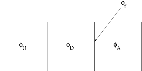
For quadrilateral and hexahedral meshes, where unique upstream and downstream faces and
cells can be identified, Ansys Fluent also provides the QUICK scheme for computing a
higher-order value of the convected variable  at a face. QUICK-type schemes [356] are based on a
weighted average of second-order-upwind and central interpolations of the variable. For the
face
at a face. QUICK-type schemes [356] are based on a
weighted average of second-order-upwind and central interpolations of the variable. For the
face  in Figure 23.4: One-Dimensional Control Volume, if the flow is from
left to right, such a value can be written as
in Figure 23.4: One-Dimensional Control Volume, if the flow is from
left to right, such a value can be written as
 | (23–7) |
 in the above equation results in a central second-order interpolation while
 yields a second-order upwind value. The traditional QUICK scheme is obtained
by setting
yields a second-order upwind value. The traditional QUICK scheme is obtained
by setting  . The implementation in Ansys Fluent uses a variable, solution-dependent
value of
. The implementation in Ansys Fluent uses a variable, solution-dependent
value of  , chosen so as to avoid introducing new solution extrema.
The QUICK scheme will typically be more accurate on structured meshes aligned with the flow direction. Note that Ansys Fluent allows the use of the QUICK scheme for unstructured or hybrid meshes as well; in such cases the usual second-order upwind discretization scheme (described in Second-Order Upwind Scheme) will be used at the faces of non-hexahedral (or non-quadrilateral, in 2D) cells. The second-order upwind scheme will also be used at partition boundaries when the parallel solver is used.
Important: The QUICK scheme is available in the pressure-based solver and when solving additional scalar equations in the density-based solver.
This third-order convection scheme was conceived from the original MUSCL (Monotone Upstream-Centered Schemes for Conservation Laws) [665] by blending a central differencing scheme and second-order upwind scheme as
 | (23–8) |
where  is defined in Equation 23–5,
  is computed using the second-order upwind scheme as described in Second-Order Upwind Scheme, and the blending factor
  is 1/3.
Unlike the QUICK scheme, which is applicable to structured hex meshes only, the MUSCL scheme is applicable to arbitrary meshes. Compared to the second-order upwind scheme, the third-order MUSCL has a potential to improve spatial accuracy for all types of meshes by reducing numerical diffusion, most significantly for complex three-dimensional flows, and it is available for all transport equations.
Important: The third-order MUSCL currently implemented in Ansys Fluent does not contain any Gradient limiter. As a result, it can produce undershoots and overshoots when the flow-field under consideration has discontinuities such as shock waves.
Important: The MUSCL scheme is available in the pressure-based and density-based solvers.
For simulations using the VOF multiphase model, upwind schemes are generally unsuitable for interface tracking because of their overly diffusive nature. Central differencing schemes, while generally able to retain the sharpness of the interface, are unbounded and often give unphysical results. In order to overcome these deficiencies, Ansys Fluent uses a modified version of the High Resolution Interface Capturing (HRIC) scheme. The modified HRIC scheme is a composite NVD scheme that consists of a nonlinear blend of upwind and downwind differencing [467].
First, the normalized cell value of volume fraction,  , is computed and is used to find the normalized face value,
  , as follows:
 | (23–9) |
where  is the acceptor cell,
  is the donor cell, and
  is the upwind cell, and
 | (23–10) |
Here, if the upwind cell is not available (for example, unstructured mesh), an
extrapolated value is used for  . Directly using this value of
  causes wrinkles in the interface, if the flow is parallel to the interface.
So, Ansys Fluent switches to the ULTIMATE QUICKEST scheme (the one-dimensional bounded version
of the QUICK scheme [355]) based on the angle between the face
normal and interface normal:
causes wrinkles in the interface, if the flow is parallel to the interface.
So, Ansys Fluent switches to the ULTIMATE QUICKEST scheme (the one-dimensional bounded version
of the QUICK scheme [355]) based on the angle between the face
normal and interface normal:
 | (23–11) |
This leads to a corrected version of the face volume fraction,  :
:
 | (23–12) |
where
 | (23–13) |
and  is a vector connecting cell centers adjacent to the face
  .
.
The face volume fraction is now obtained from the normalized value computed above as follows:
 | (23–14) |
The modified HRIC scheme provides improved accuracy for VOF calculations when compared to QUICK and second-order schemes, and is less computationally expensive than the Geo-Reconstruct scheme.
Higher order schemes can be written as a first-order scheme plus additional terms for the higher-order scheme. The higher-order relaxation can be applied to these additional terms.
The under-relaxation of high order terms follows the standard formulation for any generic
property 
 | (23–15) |
Where  is the under-relaxation factor. Note that the default value of
 for steady-state cases is 0.25 and for transient cases is 0.75. The same
factor is applied to all equations solved.
for steady-state cases is 0.25 and for transient cases is 0.75. The same
factor is applied to all equations solved.
For information about this solver option, see High Order Term Relaxation (HOTR) in the User's Guide.