For additional information, see the following sections:
Solution steering in the density-based implicit solver provides you with an expert system that will help navigate the flow solution from a starting initial guess to a converged solution with minimum user interaction. When you apply solution steering, you will be required to select the type of flow that best characterizes the solution domain and the maximum desired accuracy, and then allow the solver to take the solution to convergence. As the solver proceeds with the solution iteration, certain solver parameters will be adjusted behind the scenes to insure that a converged solution to steady-state is possible.
Important: Solution steering is available only for steady-state flows in the density-based implicit solver.
The convergence to steady-state solution is achieved in two stages. The parameters that are used in these stages are determined and set based on user input for the type of flow that can best characterize the solution domain. The type of flows available for selection are classified based on flow compressibility as well as the dominant flow Mach number in the solution domain.
The following flow types are available:
Incompressible (if the flow is incompressible, that is density is constant)
Subsonic (if the flow is compressible and M<0.75)
Transonic (if the flow is compressible and 0.65<M<1.2)
Supersonic (if the flow is compressible and 1.10< M<2.5)
Hypersonic (if the flow is compressible and 2.0< M)
Important: There is no exact Mach number cut-off for these regions, therefore, the above Mach number ranges are just a simple guideline to help you select a flow type.
Solution steering will typically perform full multigrid (FMG) initialization followed by two iterative stages. The purpose of each stage is described below.
Immediately before the start of the iteration, solution steering will perform full multigrid initialization to obtain the best possible initial starting solution.
Stage 1:
The purpose of Stage 1 is to navigate the solution from the difficult initial phase of the solution toward convergence by insuring maximum stability. During this stage, the solution is advanced gradually from 1st-order accuracy to maximum accuracy (user specified and typically 2nd-order) at a constant low CFL value.
Stage 2:
In this stage the solution is driven hard towards convergence by regular adjustments of the CFL value to insure fast convergence as well as to prevent possible divergence.
In stage 2, the residual history is monitored and analyzed through regular intervals to determine if an increase or decrease in CFL value is needed to obtain fast convergence or to prevent divergence.
Solution steering is disabled by default. However, when the following criteria are met, the solution steering feature will become available for selection:
| Feature | Setting |
|---|---|
| Solver Type | Density Based |
| Solver Formulation | Implicit |
| Time Formulation | Steady |
| Data is valid (either data file has been read or flow has been initialized) |
To turn on solution steering, enable the Solution Steering option as shown in Figure 36.65: The Run Calculation Task Page with Solution Steering Enabled.
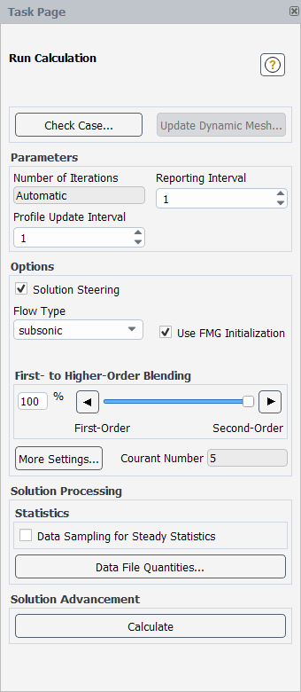
The Run Calculation task page will then expand to display the solution steering main controls (see Figure 36.65: The Run Calculation Task Page with Solution Steering Enabled). To obtain a flow solution using solution steering, you will need to perform the following:
Select the type of flow.
Select the maximum accuracy desired (first- to second-order blending).
Click .
You can also adjust the number of iterations, or customize the parameters of the solution steering if the default setting is not sufficient for the type of flow problem being solved.
Before using solution steering, you will need to prepare and set up the case as usual as described in the Getting Started part of this manual.
After Solution Steering is enabled, specify the following:
- Flow Type
allows you to select the flow type that best describes the flow in the solution domain. Five choices are available: incompressible, subsonic, transonic, supersonic, and hypersonic.
- Use FMG Initialization
when enabled allows for full multigrid initialization before starting stages 1 and 2. FMG initialization is enabled by default.
- First- to Higher-Order Blending
allows you to reduce the desired solution accuracy by selecting a blending factor less than 100%. The default setting is 100%. See First- to Higher-Order Blending in the Theory Guide for more information. The blending factor will be grayed out if Second Order Upwind discretization for the Flow equations is not selected in the Solution Methods task page. The solution accuracy may be reduced (typical values are 75% or 50%) if it is not possible to obtain a converged solution with the maximum second-order accuracy (that is blending = 100%).
- Courant Number
in the Run Calculation task page is a non-adjustable field displaying the current CFL number, which allows you to view it during the calculation.
- More Settings...
opens the Solution Steering dialog box, providing a host of settings that control the solution steering strategy, as shown in Figure 36.66: The Solution Steering Dialog Box.
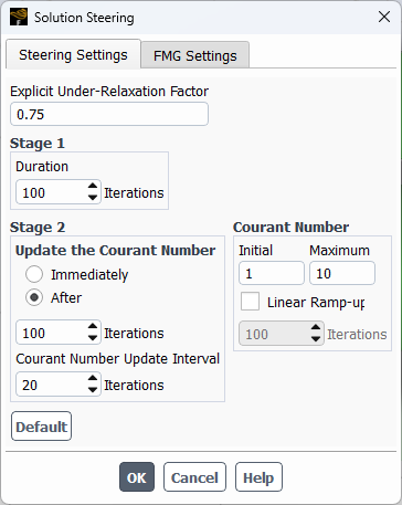
The Solution Steering dialog box, shown in Figure 36.66: The Solution Steering Dialog Box, contains two tabs. The Steering Settings tab sets the solution steering parameters and the FMG Settings sets the full multigrid initialization parameters.
In the Steering Setting tab, you can modify the parameters used in Stages 1 and 2.
- Explicit Under-Relaxation Factor
allows the solution to be under-relaxed to improve convergence. The under-relaxation value is determined by the Flow Type that you selected in the Run Calculation task page, when Solution Steering was enabled. In general, you do not need to alter the default value set in this field. Refer to Under-Relaxation of Variables in the Theory Guide for more information about explicit relaxation.
- Stage 1
Duration is the number of iterations in stage 1. The CFL number used during these iterations is set in the Initial field, in the Courant Number group box.
- Stage 2
The Courant number update in stage 2 can start immediately after the end of stage 1, or after a certain designated number of iterations. If the Courant number update is to start immediately after stage 1 then Immediately should be selected (this is the default option). If the Courant number update is desired after some lagged period of iterations, then After should be selected and the lag in the number of iterations should be entered in the field below it. The frequency at which the Courant number is updated is defined in Courant Number Update Interval field.
- Courant Number
Initial is the starting Courant number and Maximum is the maximum allowed Courant number. The solution steering algorithm will not allow the solver to exceed the maximum Courant number, but will allow the solver to use a Courant number less than the initial Courant number if divergence in the solution has occurred.
If Linear Ramp-up is selected, the active Courant number steering in stage 2 is replaced by a linear ramp-up of the CFL. The Courant number is increased from the Initial to Maximum value over a set number of iterations, determined by the Iterations field. The Courant number may be automatically reduced if divergence is detected.
- Default
is available in the Steering Settings tab to reset any changes made to the parameters to their original default values.
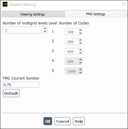
In the FMG Settings tab (Figure 36.67: The FMG Settings Tab in the Solution Steering Dialog Box), the Number of multigrid levels and Number of Cycles in each Level, as well as the FMG Courant Number used in the FMG initialization can be adjusted. The default values used in the multigrid settings are determined from the type of flow that you selected, the size of the mesh, and the flow dimensionality. The Default button is used to reset any changes to the original default values. For more information about FMG initialization, refer to Full Multigrid (FMG) Initialization.