


The thermal conductivity must be defined when heat transfer is active. You must define thermal conductivity when you are modeling energy and viscous flow.
Ansys Fluent provides several options for definition of the thermal conductivity:
constant thermal conductivity
temperature- and/or composition-dependent thermal conductivity
kinetic theory
anisotropic (anisotropic, biaxial, orthotropic, cylindrical orthotropic, principal axes and principal values, user-defined anisotropic) (for solid materials only)
user-defined
Each of these input options and the governing physical models are detailed in this section. User-defined functions (UDFs) are described in the Fluent Customization Manual.
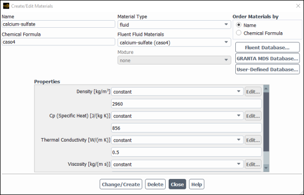
In all cases, you will define the Thermal Conductivity in the Create/Edit Materials Dialog Box (Figure 8.22: The Create/Edit Materials Dialog Box).
![]() Setup →
Setup → ![]() Materials
→ Create/Edit...
Materials
→ Create/Edit...
Thermal conductivity is defined in units of W/m-K in SI units or BTU/hr-ft-°R in British units.
For additional information, see the following sections:
- 8.5.1. Constant Thermal Conductivity
- 8.5.2. Thermal Conductivity as a Function of Temperature
- 8.5.3. Thermal Conductivity Using Kinetic Theory
- 8.5.4. Defining Thermal Conductivity Using Gupta Curve Fits
- 8.5.5. Composition-Dependent Thermal Conductivity for Multicomponent Mixtures
- 8.5.6. Anisotropic Thermal Conductivity for Solids
If you want to define the thermal conductivity as a constant, check that constant is selected in the drop-down list to the right of Thermal Conductivity in the Create/Edit Materials Dialog Box (Figure 8.22: The Create/Edit Materials Dialog Box), and enter the value of thermal conductivity for the material.
For the default fluid (air), the thermal conductivity is 0.0242 W/m-K.
You can also choose to define the thermal conductivity as a function of temperature. Three types of functions are available:


You can input the data pairs ( ), ranges and coefficients
  and
and  , or coefficients
  that describe these functions using the Create/Edit Materials Dialog Box, as described in Defining Properties Using Temperature-Dependent Functions.
If you are using the ideal gas law (as described in Density), you have the option to define the thermal conductivity using kinetic theory as
 | (8–48) |
where  is the universal gas constant,
  is the molecular weight,
  is the material’s specified or computed viscosity, and
 is the material’s specified or computed specific heat
capacity.
is the material’s specified or computed specific heat
capacity.
To enable the use of this equation for calculating thermal conductivity, select kinetic-theory from the drop-down list to the right of Thermal Conductivity in the Create/Edit Materials Dialog Box. The solver will use Equation 8–48 to compute the thermal conductivity.
When simulating hypersonic flows using the default one-temperature approach, Fluent offers Gupta curve fits that are applicable for air mixtures with temperatures up to 30 000 K. For details, see Modeling Transport Properties Using Gupta Curve Fits .
If you are modeling a flow that includes more than one chemical species (multicomponent flow), you have the option to define a composition-dependent thermal conductivity. (Note that you can also define the thermal conductivity of the mixture as a constant value or a function of temperature, or using kinetic theory.)
To define a composition-dependent thermal conductivity for a mixture, follow these steps:
For the mixture material, choose mass-weighted-mixing-law or, if you are using the ideal gas law, ideal-gas-mixing-law in the drop-down list to the right of Thermal Conductivity. If you have a user-defined function that you want to use to model the thermal conductivity, you can choose either the user-defined method or the user-defined-mixing-law method for the mixture material in the drop-down list.
The only difference between the user-defined-mixing-law and the user-defined option for specifying density, viscosity and thermal conductivity of mixture materials, is that with the user-defined-mixing-law option, the individual properties of the species materials can also be specified. Note that only the constant, the polynomial methods and the user-defined methods are available.
Important: If you use ideal-gas-mixing-law for the thermal conductivity of a mixture, you must use ideal-gas-mixing-law or mass-weighted-mixing-law for viscosity, because these two viscosity specification methods are the only ones that allow specification of the component viscosities, which are used in the ideal gas law for thermal conductivity (Equation 8–49).
Click .
Define the thermal conductivity for each of the fluid materials that make up the mixture. You may define constant or (if applicable) temperature-dependent thermal conductivities for the individual species. You may also use kinetic theory for the individual thermal conductivities, if applicable.
If you selected user-defined-mixing-law, define the thermal conductivity for each of the fluid materials that make up the mixture. You may define constant, or (if applicable) temperature-dependent thermal conductivities, or user-defined thermal conductivities for the individual species. More information about defining properties with user-defined functions can be found in the Fluent Customization Manual.
If you are using the ideal gas law, the solver will compute the mixture thermal conductivity based on kinetic theory as
 | (8–49) |
where
 | (8–50) |
and  is the mole fraction of species
  .
.
For non-ideal gases, the mixture thermal conductivity is computed based on a simple mass fraction average of the pure species conductivities:
 | (8–51) |
The anisotropic conductivity options in Ansys Fluent solves the conduction equation in solid zones and shells with the thermal conductivity specified as a matrix. The heat flux vector is written as
 | (8–52) |
The following options are available for defining anisotropic thermal conductivity in Ansys Fluent. These are discussed below.
anisotropic
biaxial (available for shells only)
orthotropic
cylindrical orthotropic
principal axes and principal values
user-defined anisotropic
Note: When postprocessing solid material properties, the Thermal Conductivity will be displayed as zero if an anisotropic thermal conductivity model is being used for a solid material. However, additional postprocessing variables are available to display the components of the thermal conductivity matrix: Thermal Conductivity XX | XY | XZ | YX | YY | YZ | ZX | ZY | ZZ. When orthotropic thermal conductivity is used, the thermal conductivity matrix is symmetric, and the following variables are not made available to avoid redundancy: Thermal Conductivity YX | ZX | ZY.
Important: The anisotropic conductivity options are available only with the pressure-based solver; you cannot use them with the density-based solvers.
For cases that have solid zones that use an anisotropic thermal conductivity option, you can change the following settings: you can select the method used to calculate the heat flux (which can affect the calculation robustness and convergence rate); you can select the method used to calculate the temperature gradient (which can affect the simulation speed); and/or you can set the relaxation for the heat flux coefficient (which can improve convergence in certain cases). For details about changing these settings, see Settings for Anisotropic Solid Zones.
For anisotropic diffusion, the thermal conductivity matrix (Equation 8–52) is specified as
 | (8–53) |
where  is the conductivity and
  is a matrix (2
  2 for two dimensions and 3
  3 for three-dimensional problems). Note that
  can be a non-symmetric matrix.
To define anisotropic thermal conductivity for a solid material, select anisotropic for Thermal Conductivity in the Create/Edit Materials Dialog Box (Figure 8.22: The Create/Edit Materials Dialog Box). Note the following:
If the principal axes of your anisotropic material are not aligned with the global coordinate system of your simulation, it may be easier for you to use one of the following options: if the axes are orthogonal, you can use the orthotropic option, as described in Orthotropic Thermal Conductivity; if the axes are not orthogonal, you can use the principal-axes-values option, as described in Principal Axes and Principal Values. If you use the anisotropic option with unaligned axes, it is your responsibility to transform the thermal conductivity properties into the
 tensor aligned with the global coordinate system.
The anisotropic option is appropriate when the components of the
 matrix are constants and do not vary independently; if this is not
the case, you can use a UDF to define the matrix and select
user-defined-anisotropic-k, as described in User-Defined Anisotropic Thermal Conductivity.
matrix are constants and do not vary independently; if this is not
the case, you can use a UDF to define the matrix and select
user-defined-anisotropic-k, as described in User-Defined Anisotropic Thermal Conductivity.
Selecting anisotropic will open the Anisotropic Conductivity Dialog Box (Figure 8.23: The Anisotropic Conductivity Dialog Box).
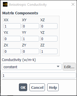
In the Anisotropic Conductivity Dialog Box, enter the Matrix
Components of matrix  and then select the Conductivity (
 in Equation 8–53) to be a
constant, polynomial function of temperature
(polynomial, piecewise-linear,
piecewise-polynomial), or user-defined function.
See Constant Thermal Conductivity and Thermal Conductivity as a Function of Temperature for details on constants and thermal polynomial
functions.
in Equation 8–53) to be a
constant, polynomial function of temperature
(polynomial, piecewise-linear,
piecewise-polynomial), or user-defined function.
See Constant Thermal Conductivity and Thermal Conductivity as a Function of Temperature for details on constants and thermal polynomial
functions.
When you select the user-defined option, the User-Defined Functions Dialog Box will open, allowing you to hook a
DEFINE_PROPERTY UDF only if you have
previously loaded a compiled UDF library or interpreted the UDF. Otherwise, you will get
an error message. Details about user-defined functions can be found in the Fluent Customization Manual.
Biaxial thermal conductivity is applicable only for solid materials used for the wall shell conduction model. To define a biaxial thermal conductivity, select biaxial in the drop-down list for Thermal Conductivity in the Create/Edit Materials Dialog Box. This opens the Biaxial Conductivity Dialog Box (Figure 8.24: The Biaxial Conductivity Dialog Box).
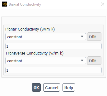
In the Biaxial Conductivity Dialog Box, both the conductivity normal to the surface of the shell (Transverse Conductivity) and the conductivity parallel to the surface of the shell (Planar Conductivity) can be defined as constant, polynomial, piecewise-linear, or piecewise-polynomial. See Constant Thermal Conductivity and Thermal Conductivity as a Function of Temperature for details on these parameters. Note that the Planar Conductivity is isotropic. See Figure 16.10: The Conduction Manager Dialog Box.
When the orthotropic thermal conductivity is used, the thermal conductivities
 in the principal directions
  are specified. The conductivity matrix is then computed as
 | (8–54) |
To define an orthotropic thermal conductivity in solids, select orthotropic in the drop-down list for Thermal Conductivity in the Create/Edit Materials Dialog Box. This opens the Orthotropic Conductivity Dialog Box (Figure 8.25: The Orthotropic Conductivity Dialog Box).
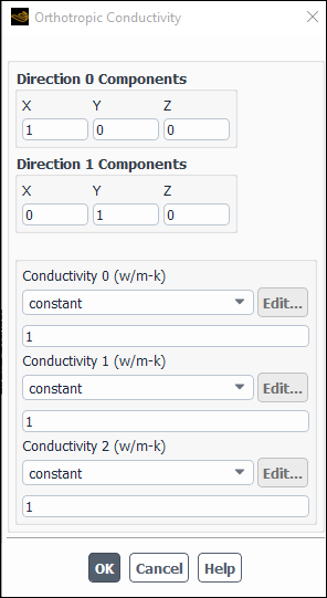
Since the directions  are mutually orthogonal, only the first two need to be specified for
three-dimensional problems.
are mutually orthogonal, only the first two need to be specified for
three-dimensional problems.  is defined using X, Y, Z under Direction
0 Components, and
is defined using X, Y, Z under Direction
0 Components, and  is defined using X, Y, Z under Direction
1 Components. You can define Conductivity 0
is defined using X, Y, Z under Direction
1 Components. You can define Conductivity 0
 , Conductivity 1
  , and Conductivity 2
  as constant, polynomial,
piecewise-linear, piecewise-polynomial functions
of temperature, user-defined, expression, or as
a New Input Parameter. See Constant Thermal Conductivity and Thermal Conductivity as a Function of Temperature for details on constant and temperature profile
functions.
as constant, polynomial,
piecewise-linear, piecewise-polynomial functions
of temperature, user-defined, expression, or as
a New Input Parameter. See Constant Thermal Conductivity and Thermal Conductivity as a Function of Temperature for details on constant and temperature profile
functions.
When you select the user-defined option, the User-Defined Functions Dialog Box will open, allowing you to hook a
DEFINE_PROPERTY UDF only if you have
previously loaded a compiled UDF library or interpreted the UDF. Otherwise, you will get
an error message. More information about user-defined functions can be found in the Fluent Customization Manual.
When you select the expression option, the Expression Dialog Box will open, allowing you to define an expression for each of the conductivity component fields. Refer to Fluent Expressions Language for more information on defining expressions.
When you select the New Input Parameter option, the
Parameter Expression dialog box will open as described in Defining and Viewing Parameters. Note that to specify an orthotropic conductivity as an
input parameter though the TUI, you must first use the command
define/parameters/enable-in-TUI? yes.
Important: For two-dimensional problems, only the functions  and the unit vector
  need to be specified.
The orthotropic conductivity of solids can be specified in cylindrical coordinates. To define the orthotropic thermal conductivity in cylindrical coordinates, select cyl-orthotropic in the drop-down list for Thermal Conductivity in the Create/Edit Materials Dialog Box. This opens the Cylindrical Orthotropic Conductivity Dialog Box (Figure 8.26: The Cylindrical Orthotropic Conductivity Dialog Box).
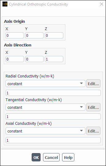
In three-dimensional cases, the origin and the direction of the cylindrical coordinate system must be specified along with the radial, tangential, and axial direction conductivities. In two-dimensional cases, the origin of the cylindrical coordinate system must be specified along with the radial and tangential direction conductivities. Note that in two-dimensional cases, the direction is always along the +Z axis. Ansys Fluent will automatically compute the anisotropic conductivity matrix at each cell from this input. The calculation is based on the location of the cell in the cylindrical coordinate system specified.
You can define the Radial Conductivity, Tangential Conductivity, and Axial Conductivity as constant, polynomial, piecewise-linear, piecewise-polynomial, or as user-defined functions of temperature. See Constant Thermal Conductivity and Thermal Conductivity as a Function of Temperature for details on constant and thermal profile functions.
When you select the user-defined option, the User-Defined Functions Dialog Box will open, allowing you to hook a
DEFINE_PROPERTY UDF only if you have
previously loaded a compiled UDF library or interpreted the UDF. Otherwise, you will get
an error message. More information about user-defined functions can be found in the Fluent Customization Manual.
Important: For conductivity calculations near the wall, the cell next to the wall is chosen for computing the conductivity matrix instead of the wall itself.
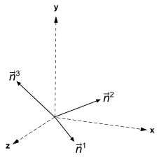
When the principal axes of your anisotropic material are not aligned with the global
coordinate system of the simulation, you can define the thermal conductivity using the
components of these axes ( ,
,  , and for 3D problems,
  ) and the associated principle values (
 ,
,  , and for 3D problems,
  ). The axes take the following form:
 | (8–55) |
Note that while the axes must be linearly independent vectors, they do not have to be unit vectors or orthogonal.
An example of principal axes that are not aligned with the global coordinate system is shown in Figure 8.27: Unaligned Principal Axes.
Representing the thermal conductivity matrix ( in Equation 8–52) in matrix notation
(
in Equation 8–52) in matrix notation
( ), the following equation is used by Ansys Fluent to transform the principal
axes and principal values into the correct tensor form:
), the following equation is used by Ansys Fluent to transform the principal
axes and principal values into the correct tensor form:
 | (8–56) |
The matrices in the previous equation are defined as follows:
 | (8–57) |
 | (8–58) |
where  is the conductivity.
To use principal axes and principal values to define the anisotropic thermal conductivity for your solid material, select principal-axes-values for Thermal Conductivity in the Create/Edit Materials Dialog Box (Figure 8.22: The Create/Edit Materials Dialog Box). This will open the Anisotropic Conduction - Principal Components Dialog Box (Figure 8.28: The Anisotropic Conductivity - Principal Components Dialog Box).
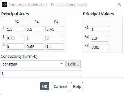
In the Principal Axes group box of the Anisotropic Conduction - Principal Components Dialog Box, enter the
i, j, and k components for
each of the n1, n2, and n3
vectors (Equation 8–55) that define the principal axes of
your material in the global coordinate system; note that these must be linearly
independent vectors. Then in the Principal Values group box, enter
the K1, K2, and K3 values
that define the magnitudes of the principal values along the associated principal axes.
Finally, make a selection from the Conductivity drop-down menu to
specify  (in Equation 8–58) as a
constant, polynomial function of temperature
(polynomial, piecewise-linear,
piecewise-polynomial), or user-defined function,
and then define it using the number-entry box that becomes available or the dialog box
that opens. See Constant Thermal Conductivity and Thermal Conductivity as a Function of Temperature for details on constants and thermal
functions.
(in Equation 8–58) as a
constant, polynomial function of temperature
(polynomial, piecewise-linear,
piecewise-polynomial), or user-defined function,
and then define it using the number-entry box that becomes available or the dialog box
that opens. See Constant Thermal Conductivity and Thermal Conductivity as a Function of Temperature for details on constants and thermal
functions.
When you select the user-defined option, the User-Defined Functions Dialog Box will open, allowing you to hook a
DEFINE_PROPERTY UDF only if you have
previously loaded a compiled UDF library or interpreted the UDF. Otherwise, you will get
an error message. Details about user-defined functions can be found in the Fluent Customization Manual.
You have the option of modeling anisotropic conduction for domains where the
components of the thermal conductivity matrix ( in Equation 8–53) are not constants and vary
independently, perhaps as a function of space or because the domain has many anisotropic
materials stitched together to form a composite. To use this option, you must first define
the conductivity matrix using a UDF, as described in
in Equation 8–53) are not constants and vary
independently, perhaps as a function of space or because the domain has many anisotropic
materials stitched together to form a composite. To use this option, you must first define
the conductivity matrix using a UDF, as described in DEFINE_ANISOTROPIC_CONDUCTIVITY in the Fluent Customization Manual.
After you have interpreted or compiled the
DEFINE_ANISOTROPIC_CONDUCTIVITY UDF, you must then select
user-defined-anisotropic-k for Thermal
Conductivity in the Create/Edit Materials Dialog Box. This will
open the User-Defined Functions Dialog Box, which you can use to hook the
UDF.