


Composites are somewhat more difficult to model than an isotropic material such as iron or steel. Because each layer may have different orthotropic material properties, you must exercise care when defining the properties and orientations of the various layers.
The following composite modeling topics are available:
The following element types are available for modeling layered composite materials: SHELL181, SHELL281, SHELL208, SHELL209, ELBOW290, SOLSH190, SOLID185 Layered Solid, and SOLID186 Layered Solid.
The element that you select depends upon your application and the type of results that must be calculated. See the individual element descriptions to determine if a specific element can be used in your product. All layered elements allow failure-criterion calculations.
SHELL181 -- Finite Strain Shell
A four-node 3D shell element with six degrees of freedom at each node. The element has full nonlinear capabilities including large strain. The layer information is input using the section commands (SEC
xxxxx) rather than real constants. Failure criteria are available via FC and other FCxxxcommands.SHELL281 -- Finite Strain Shell
An eight-node shell element with six degrees of freedom at each node. The element is suitable for analyzing thin to moderately-thick shell structures and is appropriate for linear, large rotation, and/or large strain nonlinear applications. The layer information is input via the section commands (SEC
xxxxx) rather than real constants. Failure criteria are available via FC and other FCxxxcommands.SHELL208 -- Finite Strain Axisymmetric Shell
A two-node element with three degrees of freedom at each node: translations in the x, and y directions, and rotation about the z axis. A fourth translational degree of freedom in z direction can be included to model uniform torsion. The element has full nonlinear capabilities including large strain and is suitable for modeling thin to moderately thick axisymmetric shell structures. The layer information is input via the section commands (SEC
xxxxx). Failure criteria are available via FC and other FCxxxcommands.SHELL209 -- Finite Strain Axisymmetric Shell
A three-node element with three degrees of freedom at each node: translations in the x and y directions, and rotation about the z axis. A fourth translational degree of freedom in the z direction can be included to model uniform torsion. The element has full nonlinear capabilities including large strain and is suitable for modeling thin to moderately thick axisymmetric shell structures. The layer information is input via the section commands (SEC
xxxxx). Failure criteria are available via FC and other FCxxxcommands.ELBOW290 -- Elbow
A quadratic three-node 3D pipe element, suitable for analyzing tubular structures with thin to moderately thick walls and appropriate for linear, large rotation, and/or large strain nonlinear applications. The wall layer information is input via the section commands (SEC
xxxxx). Failure criteria are available via FC and other FCxxxcommands.SOLSH190 -- Layered Structural Solid Shell
An eight-node 3D solid shell element with three degrees of freedom per node (UX, UY, UZ). The element can be used for simulating shell structures with a wide range of thickness (from thin to moderately thick). The element has full nonlinear capabilities including large strain. The layer information is input using the section commands rather than real constants. The element can be stacked to model through-the-thickness discontinuities. Failure criteria are available via FC and other FC
xxxcommands.SOLID185 Layered Solid -- Layered Structural Solid
An eight-node 3D Layered Solid used for 3D modeling of solid structures. It is defined by eight nodes having three degrees of freedom at each node: translations in the nodal x, y, and z directions. The element has plasticity, hyperelasticity, stress stiffening, creep, large deflection, and large strain capabilities. It also has mixed formulation capability for simulating deformations of nearly incompressible elastoplastic materials, and fully incompressible hyperelastic materials. The element accommodates prism and tetrahedral degenerations when used in irregular regions. Various element technologies such as B-bar, uniformly reduced integration, and enhanced strains are supported. Failure criteria are available via FC and other FC
xxxcommands. A companion thermal element is SOLID278.SOLID186 Layered Solid -- Layered Structural Solid
A higher-order version of SOLID185. A companion thermal element is SOLID279.
In addition to the layered elements described above, other composite element capabilities are available, but are not considered further here:
The most important characteristic of a composite material is its layered configuration. Each layer may be made of a different orthotropic material and may have its principal directions oriented differently. For laminated composites, the fiber directions determine layer orientation.
Specify individual layer properties to define the layered configuration.
The following topics related to defining the layered configuration are available:
With this method, the layer configuration is defined layer-by-layer from bottom to top. The bottom layer is designated as layer 1, and additional layers are stacked from bottom to top in the positive Z (normal) direction of the element coordinate system. You need to define only half of the layers if stacking symmetry exists.
At times, a physical layer will extend over only part of the model. In order to model continuous layers, these dropped layers may be modeled with zero thickness. Figure 11.1: Layered Model Showing Dropped Layer shows a model with four layers, the second of which is dropped over part of the model.

For each layer, the following properties are specified in the element real constant table (R, RMORE, RMODIF) accessed with REAL attributes:
Material properties (via a material reference number MAT)
Layer orientation angle commands (THETA)
Layer thickness (TK)
You can also define layered sections via the Section Tool . For each layer, the following are specified in the section definition via the section commands (SECTYPE, SECDATA) or the Section Tool accessed with the SECNUM attributes.
Material properties (via a material reference number MAT)
Layer orientation angle commands (THETA)
Layer thickness (TK)
Number of integration points per layer (NUMPT)
Layer Property Descriptions
Following is more information about each of the layer properties:
Material Properties -- As with any other element, the MP command defines the linear material properties, and the TB command is used to define the nonlinear material data tables. The only difference is that the material attribute number for each layer of an element is specified in the element's real constant table. For the layered elements, the MAT command attribute is used only for the BETD, ALPD, DMPR, DMPS, and REFT arguments of the MP command. The linear material properties for each layer may be either isotropic or orthotropic. Typical fiber-reinforced composites contain orthotropic materials and these properties are most often supplied in the major Poisson's ratio form. Material property directions are parallel to the layer coordinate system, defined by the element coordinate system and the layer orientation angle.
Layer Orientation Angle -- Defines the orientation of the layer coordinate system with respect to the element coordinate system. It is the angle (in degrees) between X-axes of the two systems. By default, the layer coordinate system is parallel to the element coordinate system. All elements have a default coordinate system which you can change using the ESYS element attribute (ESYS) . You may also write your own subroutines to define the element and layer coordinate systems (USERAN and USANLY); for more information, see the Guide to User-Programmable Features in the Programmer's Reference.
Layer Thickness -- If the layer thickness is constant, you only need to specify TK(I), the thickness at node I. Otherwise, the thicknesses at the four corner nodes must be input. Dropped layers may be represented with zero thickness.
Number of integration points per layer -- Allows you to determine in how much detail the program should compute the results. For very thin layers, when used with many other layers, one point would be appropriate. But for laminates with few layers, more would be needed. The default is three points. This feature applies only to sections defined via the SEC
xxxxxsection commands.
Sandwich structures have two thin faceplates and a thick, but relatively weak, core. Figure 11.2: Sandwich Construction illustrates sandwich construction.

You can model sandwich structures with SHELL181 or SHELL281; however, both elements model the transverse-shear deflection using an energy-equivalence method that makes the need for a sandwich option unnecessary.
For SHELL181 and SHELL281
using sections defined via the section commands
(SECxxxxx), nodes can be offset during the
definition of the section via the SECOFFSET command.
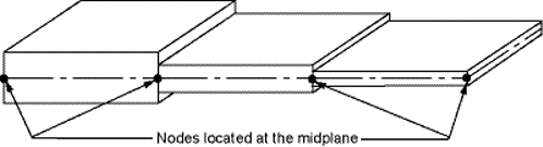
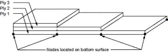
The figures below illustrate how you can conveniently model ply drop-off in shell elements that are adjacent to each other. In Figure 11.3: Layered Shell With Nodes at Midplane, the nodes are located at the middle surfaces and these surfaces are aligned. In Figure 11.4: Layered Shell With Nodes at Bottom Surface, the nodes are located at the bottom surfaces and these surfaces are aligned.
Failure criteria are used to learn if a layer has failed due to the applied loads. Three predefined failure criteria options are available; alternatively, you can specify up to six failure criteria of your own (user-written criteria). The predefined criteria are:
Maximum Strain Failure Criterion-- Allows nine failure strains.
Maximum Stress Failure Criterion -- Allows nine failure stresses.
Tsai-Wu Failure Criterion -- Allows nine failure stresses and three additional coupling coefficients.
The failure strains, stresses, and coupling coefficients may be temperature-dependent. For details about the data required for each criterion, see the Element Reference .
Failure criteria are orthotropic, so you must input the failure stress or failure strain values for all directions. (The exception is that compressive values default to tensile values.)
If you do not want the failure stress or strain to be checked in a particular direction, specify a large number in that direction.
The following topics for specifying failure criteria for composites are available:
For more information, see Failure Criteria in the Mechanical APDL Theory Reference.
To specify a failure criterion, use the family of FC commands. These FC commands can be used for any 2D or 3D structural solid element or any 3D structural shell element: FC, FCDELE, and FCLIST.
A typical sequence of commands to specify a failure criterion using these commands follows:
FC,1,TEMP,,   100,   200  ! Temperatures
FC,1,S,XTEN, 1500,  1200  ! Maximum stress components
FC,1,S,YTEN,  400,   500
FC,1,S,ZTEN,10000,  8000
FC,1,S,XY  ,  200,   200
FC,1,S,YZ  ,10000,  8000
FC,1,S,XZ  ,10000,  8000
FCLIST,      ,100         ! List status of Failure Criteria at 100.0 degrees
FCLIST,      ,150         ! List status of Failure Criteria at 150.0 degrees
FCLIST,      ,200         ! List status of Failure Criteria at 200.0 degrees
PRNSOL,S,FAIL             ! Use Failure Criteria
You can specify user-written failure criteria via user subroutine
USERFC. This subroutine should be linked with the
program beforehand. For more information, see User-Programmable Features and Nonstandard Uses in the Advanced Analysis Guide.
Following are a few helpful hints and tips for modeling and postprocessing composite elements:
- 11.1.4.1. Dealing with Coupling Effects
- 11.1.4.2. Obtaining Accurate Interlaminar Shear Stresses
- 11.1.4.3. Verifying Your Input Data
- 11.1.4.4. Specifying Results File Data
- 11.1.4.5. Selecting Elements with a Specific Layer Number
- 11.1.4.6. Specifying a Layer for Results Processing
- 11.1.4.7. Transforming Results to Another Coordinate System
Composites exhibit several types of coupling effects, such as coupling between bending and twisting, coupling between extension and bending, etc. This is due to stacking of layers of differing material properties. As a result, if the layer stacking sequence is not symmetric, you may not be able to use model symmetry even if the geometry and loading are symmetric, because the displacements and stresses may not be symmetric.
Interlaminar shear stresses are usually important at the free edges of a model. For relatively accurate interlaminar shear stresses at these locations, the element size at the boundaries of the model should be approximately equal to the total laminate thickness. For shells, increasing the number of layers per actual material layer does not necessarily improve the accuracy of interlaminar shear stresses. Interlaminar transverse-shear stresses in shell elements are based on the assumption that no shear is carried at the top and bottom surfaces of the element. These interlaminar shear stresses are only computed in the interior and are not valid along the shell element boundaries. Use of shell-to-solid submodeling is recommended to accurately compute all of the free edge interlaminar stresses.
Because a large amount of input data is necessary for composites, it is a good idea to verify the data before proceeding with the solution. The following commands are available for this purpose:
ELIST -- Lists the nodes and attributes of all selected elements.
EPLOT -- Displays all selected elements. Using the /ESHAPE,1 command before EPLOT causes shell elements to be displayed as solids with the layer thicknesses obtained from real constants or section definition (see Figure 11.5: Example of an Element Display.
/PSYMB,LAYR,n followed by EPLOT -- Displays layer number n for all selected layered elements. Use this method to display and verify each individual layer across the entire model. To use /PSYMB,LAYR with smeared reinforcing elements (REINF265), first set the vector-mode graphics option (/DEVICE,VECTOR,1).
/PSYMB,ESYS,1 followed by EPLOT -- Displays the element coordinate system triad for those elements whose default coordinate system has been changed.
LAYPLOT -- Displays the layer stacking sequence from real constants in the form of a sheared deck of cards. (See Figure 11.6: Sample LAYPLOT Display for [45/-45/ - 45/45] Sequence.) The layers are crosshatched and color coded for clarity. The hatch lines indicate the layer angle (real constant THETA) and the color indicates layer material number (MAT). You can specify a range of layer numbers for the display.
SECPLOT -- Displays the section stacking sequence from sections in the form of a sheared deck of cards. (See Figure 11.6: Sample LAYPLOT Display for [45/-45/ - 45/45] Sequence.) The sections are crosshatched and color coded for clarity. The hatch lines indicate the layer angle (THETA) and the color indicates layer material number (MAT) defined by the SECDATA command. You can specify a range of layer numbers for the display.
By default, only data for the bottom of the first (bottom) layer and top of the last (top) layer are written to the results file. If you are interested in data for all layers, set KEYOPT(8) = 1. Be aware, though, that this may result in a large results file.
![Sample LAYPLOT Display for [45/-45/ - 45/45] Sequence](graphics/GSTR11-6.svg)
Use the ESEL,S,LAYER command to select elements that have a certain layer number. If an element has a zero thickness for the requested layer, the element is not selected.
For energy output, the results are applicable only to the entire element. You cannot get output results for individual layers.
Use the LAYER command (in the POST1 postprocessor) or the LAYERP26 (in the POST26 postprocessor) to specify the layer number for which results should be processed.
The SHELL command specifies a TOP, MID, or BOT location within the layer.
The default in POST1 is to store results for the bottom of the bottom layer, and the top of the top layer, and the layer with the maximum failure criterion value. In POST26, the default is layer 1.
If KEYOPT(8) = 1 (data stored for all layers), the LAYER and LAYERP26 commands store the TOP and BOT results for the specified layer number. MID values are then calculated by average TOP and BOT values.
If KEYOPT (8) = 2 is set for SHELL181 or SHELL281 during SOLUTION, then LAYER and LAYERP26 commands store the TOP, BOTTOM, and MID results for the specified layer number. In this case, MID values are directly retrieved from the results file. For transverse-shear stresses with KEYOPT(8) = 0, therefore, POST1 can only show a linear variation, whereas the element solution printout or KEYOPT(8) = 2 can show a parabolic variation.
By default, the POST1 postprocessor displays all results in the global Cartesian coordinate system. Issue the RSYS command to transform the results to a different coordinate system. In particular, RSYS,SOLU enables you to display results in the layer coordinate system if LAYER is issued with a nonzero layer number.