


Two harmonic analysis (forced response) methods are available for cyclic structures: full and mode-superposition harmonic analysis. The advantages of the full method are:
You do no need to choose frequencies and mode shapes that adequately represent the response.
The non-cyclically symmetric loading can be arbitrary and may be applied to any sector.
The advantages of the mode-superposition method are:
It is faster than the full method.
Postprocessing is more encompassing.
Only engine order loading (traveling wave excitation) is supported in a mode-superposition analysis. Cyclically symmetric loading is a special case of engine order loading where the engine order is equal to zero.
While engine order excitation is a non-cyclically symmetric load, no other forms of non-cyclically symmetric loads are supported.
Cyclically symmetric or non-cyclically symmetric loading may be applied in a full harmonic cyclic analysis.
Fluid-structure interaction (FSI) is supported for full harmonic cyclic symmetry analysis when acoustic elements are present. See Using Cyclic Symmetry with Fluid-Structure Interaction in the Acoustic Analysis Guide for a list of supported element types and other details.
Constraint and joint elements (MPC184) are not supported for full linear perturbation harmonic cyclic symmetry analyses.
The flowchart below illustrates the process involved in a harmonic cyclic symmetry analysis with non-cyclically symmetric loading.
Figure 4.7: Process Flow for a Full Harmonic Cyclic Symmetry Analysis (Non-cyclically Symmetric Loading)
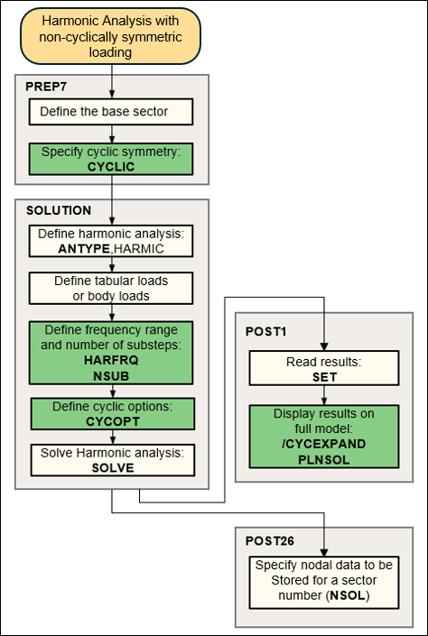
For more information, see Non-Cyclically Symmetric Loading
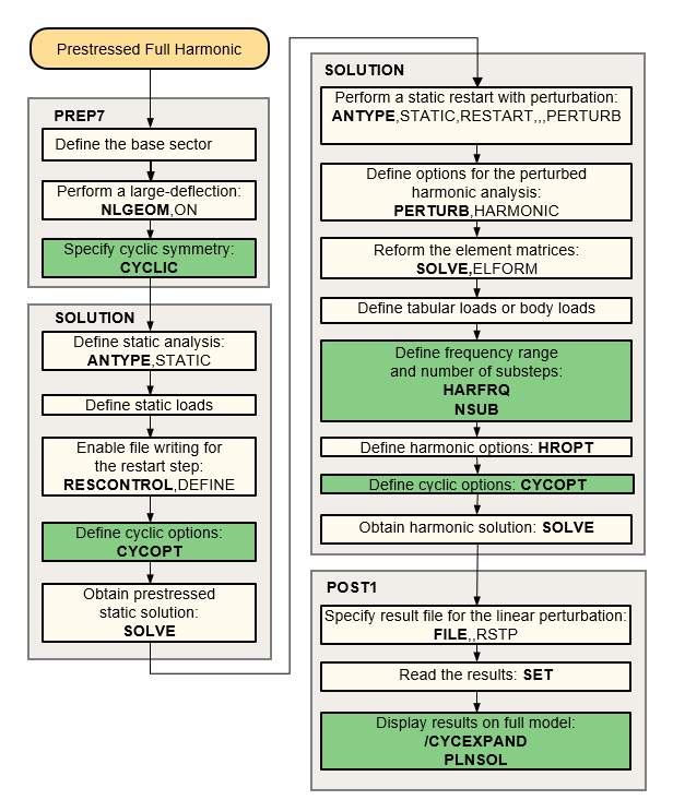
The process for solving a prestressed harmonic cyclic symmetry analysis is essentially the same as a stress free case, except that a static solution is necessary to calculate the prestress in the base sector. The prestress state of the sector may be from a linear static or a large-deflection nonlinear static analysis. Non-cyclically symmetric loading cannot be applied in the static solution.
The linear perturbed harmonic cyclic symmetric analysis is supported for the following methods: AUTO, FULL, VT (see HROPT command).
Cyclic or non-cyclically symmetric loading may be applied in a prestressed full harmonic cyclic analysis.
The flowchart below illustrates the process of a harmonic cyclic symmetry analysis with non-cyclically symmetric loading.
If cyclic expansion via the /CYCEXPAND command is active, the PLNSOL and PRNSOL commands have summation of all required harmonic index solutions by default.
In a full harmonic analysis with non-cyclically symmetric loading, all applicable harmonic index solutions are computed and saved in the results file as load step results.
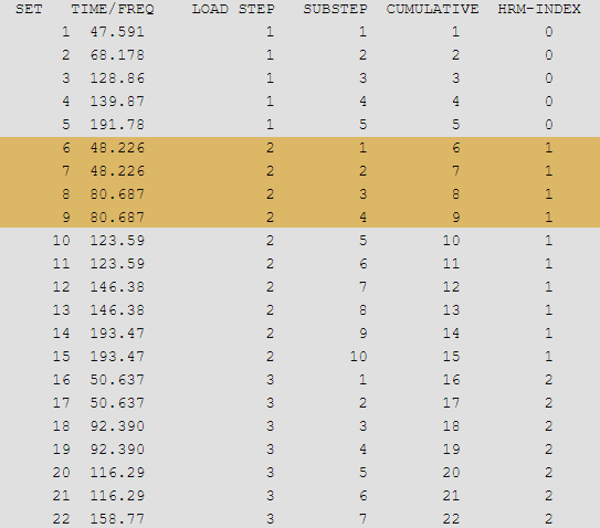
A SET,LIST command lists the range of load step numbers in the group containing each solution. Each load step post data header contains the first, last, and count of load steps from the given SOLVE command, as shown:
        *****  INDEX OF DATA SETS ON RESULTS FILE  *****
SET  TIME/FREQ  LOAD STEP  SUBSTEP  CUMULATIVE  HRM-INDEX  GROUP
1    1.0000     1          1        1           0          1-3
2    2.0000     2          1        2           1          1-3
3    3.0000     3          1        3           2          1-3
4    1.0000     1          1        1           0          4-6
5    2.0000     2          1        2           1          4-6
6    3.0000     3          1        3           2          4-6
...
The SET command establishes which SOLVE load step group should display. Summation via /CYCEXPAND is automatic. Plots and printed output show the summation status.
With /CYCEXPAND turned on, the results are expanded at each
load step and then combined to plot the full solution as a complete sum. For
example, in a four sector model where the harmonic index results 0 through 2 are
available in the results file, the plot command PLNSOL will
display the results as STEP=1 THRU=3 COMPLETE
SUM.
Accumulation occurs at the first applicable PLNSOL or PRNSOL command. After accumulation, the last load step number of the current group becomes the new current load step number.
Amplitude results are available for component results (e.g. UX, SX) using /CYCEXPAND,,PHASEANG,AMPL. Amplitude results for non-component results (e.g. USUM, SEQV) are not available using full harmonic cyclic symmetry. To compute non-component results, you can use mode-superposition harmonic cyclic symmetry or cyclic symmetry in the Mechanical Application. Note that using SET,,,,AMPL is not valid in cyclic symmetry analysis.
Use the POST26 time-history postprocessor
(/POST26) to view cyclic symmetry results as a function
of frequency. Input the sector number for which results are needed on the
NSOL command
(NSOL,,,,,,SECTOR). The
NSOL labels supported for cyclic symmetry analyses are
UX, UY, UY, ROTX, ROTY, ROTZ, and PRES. The results are shown in the solution
coordinate system. Note that POST26 results for cyclic symmetry are only valid
when the solution coordinate system is aligned with the cyclic coordinate
system.
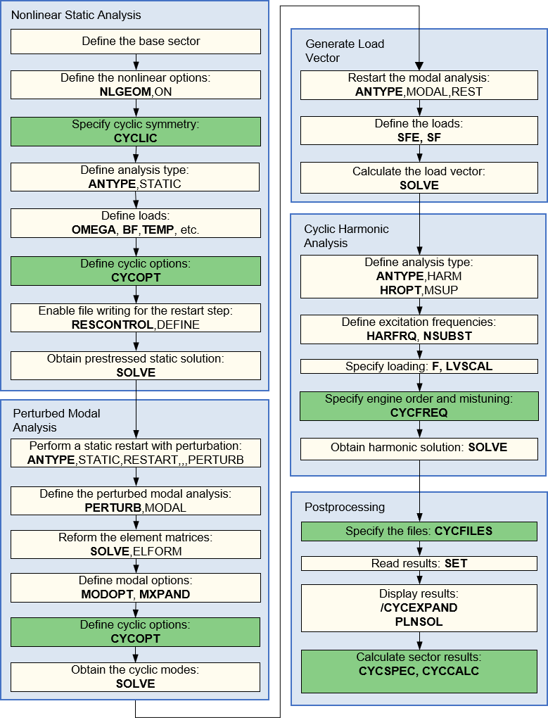
The mode-superposition (MSUP) method sums factored mode shapes (obtained from a modal analysis) to calculate the harmonic response. The procedure (in the most general case) consists of these steps:
Build the cyclic model (matched cyclic edge nodes only)
Perform a static cyclic symmetry analysis to obtain the prestressed state
Perform a linear perturbation modal cyclic symmetry analysis
Restart the modal analysis to create the desired load vector from any element loads (for example, pressures)
Apply additional nodal loads, scale previously formed loads, and apply modal loads in the harmonic solution step.
Obtain the mode-superposition harmonic cyclic symmetry solution, including mistuning and aero effects if desired.
The following flowchart illustrates the process involved in a prestressed mode-superposition harmonic cyclic symmetry analysis. For a non-prestressed solution, you may skip step 2, so that step 3 becomes a stress-free modal analysis.
The first step, building the cyclic model, is described in Cyclic Modeling. Note that only matched cyclic edge nodes may be used. The remaining steps are described below.
Static Cyclic Symmetry Analysis describes how to obtain the static solution that will compute the prestressing. In the static analysis:
Only cyclically symmetric loading is permitted
You cannot use CYCOPT,MSUP,OFF as this is the non-default setting.
This step is outlined in Large-Deflection Prestressed Modal Cyclic Symmetry Analysis, and has the following restrictions and guidelines:
Only Block Lanczos is supported (MODOPT,LANB).
You must use MXPAND to write the modes to the results file.
The frequency range on MXPAND is ignored. Specify the frequency range using the MODOPT command instead.
Be sure to extract all the modes that may contribute to the harmonic response. As a general guideline, modes contributing to the harmonic response will fall in the range ½Ω to 2Ω, where Ω is the harmonic frequency (HARFRQ) used in the subsequent harmonic solution. If mistuned, a range of ½Ω to 5Ω is recommended.
Residual vectors (RESVEC) are not supported.
Enforced motion (MODCONT,,ON) is not supported.
Mode selection is not supported.
Stress modes (MXPAND,ALL,,,YES,,YES) are not supported.
An even number of modes (per harmonic index) is always computed. If you specify an odd number of modes on the MODOPT command, it is increased by 1.
You may use ANPRES to animate the pressure loading at the specified engine order (CYCFREQ,EO).
If you need to apply harmonically varying elements loads (for example, pressures), specify them in the modal analysis. The program ignores the loads for the modal solution but calculates a load vector and writes it to the mode shape file (Jobname.mode). You can also generate multiple load vectors. The load vectors created can then be scaled and used in the harmonic solution. For more information, see Modal Analysis Restart in the Basic Analysis Guide. The following limitations apply:
You may not introduce additional elements (such as SURF154) to facilitate application of the loads. You must apply the loads directly to the existing base elements and nodes. Specify any load elements in the static step (or prior to the modal solution if there is no prestressing step required) before the CYCLIC command is issued.
Nodal loads (F) can be applied directly in the harmonic analysis if desired, rather than creating a modal load vector.
Specify THEXPAND,OFF to ignore the thermal loads in the load vector generation.
Loads cannot be applied on nodes on the cyclic boundaries or on elements that lie on or adjacent to the cyclic boundary.
It is possible to skip this step and add the loads directly in the prior modal analysis step. If you choose to skip this step, only one modal load vector can be generated.
You may use the /MAP processor to map pressure loads from a CFD analysis, and from a CFX Transient Blade Row analysis in particular, to use in the harmonic analysis. See Unidirectional Pressure Mapping: CFD to Mechanical APDL in the Coupled-Field Analysis Guide.
In the harmonic response solution step, it is possible to apply modal loads directly. Modal loads could be any load that has already been projected into the modal space and is associated with a known mode of the model (for example, pressure loads from a CFD analysis that were determined and then projected onto a mode of the system, all within the CFD workflow). These modal loads can be applied when other loads have been specified, and all loads applied will act upon the structure. This capability significantly saves time and improves accuracy by eliminating the need to map CFD based loads onto the mechanical structure.
Note: It is important to remember that cyclic symmetry modes from the exact same model can change (i.e. clocking/orientation), depending on factors such as the number of frequencies requested or the hardware used to run the software. Therefore, it is critical to include only the modes that will be used in the cyclic mode-superposition (MSUP) harmonic solution. Failure to do so could result in modal loads that are inconsistent with the cyclic MSUP model.
To apply a modal load, you must create an MAPDL array of modal loads, ordered
to reflect the order of modes kept in the harmonic response analysis.
Unspecified modal loads within the array are given a zero value. In the case of
mistuning (CYCFREQ,MIST), all modes from the modal solve are
kept. Instead, for tuned systems, only modes that correspond to the harmonic
index excited by the loading engine order (set by
CYCFREQ,EO,Value1) are kept.
The following example demonstrates this concept and shows a command snippet that
applies modal loads directly using a modal load array.
Example 4.1: Apply Modal Loads Directly Using an Ordered Array
/solu
antype,harmonic
hropt,msup,
outres,all,all
harfrq,30,60
nsubs,30,30,30

! Create Modal Load Array
*dim,MdLd,array,4,2  ! Set the Modal Load Array Dimensions
MdLd(1,1) = 3.56, 0.0 , 6.22 , 4.55  ! Real Part Modal Load
MdLd(1,2) = 1.53 , 0.0 , 2.29 , 3.83 ! Imag Part Modal Load
! Apply Modal Load
cycfreq,eo,1,MdLd
Of the modes computed in the modal analysis listed below, only those highlighted have modal loads applied. Because an engine order of 1 was specified on the CYCFREQ,EO command, the program only excites harmonic index 1 modes. The dimension of the modal load array prescribes that only the first four modes in that load step have modal loads applied, and of these, the second array value sets the modal load to 0.0 for the second mode in the second load step.
In this step, the program uses mode shapes extracted by the modal solution to calculate the harmonic response. The following requirements apply:
The mode shape file (Jobname.mode) must be available.
The full file (Jobname.full) must be available.
The database must contain the same model from which the modal solution was obtained.
Additionally, the following limitations apply:
The range of modes on the HROPT command is ignored. All the modes from the modal analysis are considered.
Tabular loading with respect to frequency is not supported in the cyclic symmetry mode-superposition harmonic solution. Only tabular loading with respect to location is supported.
When using the NSUBST command, the
NSBMX,NSBMN, andCarryarguments are not supported.
The following inputs must also be provided:
Apply the required load on the base sector. Nodal forces and the load vector created in the modal analysis are valid. Use the LVSCALE command to apply the load vector from the modal solution. Note that all loads from the modal analysis are scaled, including forces and pressures. To avoid load duplication, delete any loads that were applied in the modal analysis.
Apply any previously computed modal loads. Modal loads can be applied in conjunction with loads applied on the mesh. Regardless of how the load is applied (direct nodal loads in the harmonic solve, loads assembled in a modal restart and specified in the harmonic solve, or direct modal loads), all applied loads will act upon the structure.
Specify the engine order of the excitation (CYCFREQ,EO). Typically, the engine order is simply a count of the number of stators, combustion nozzles, etc., that cause the disturbance. All loads from the modal solution and nodal loads that are applied during a given load step will be applied as engine order loads. The program computes the “aliased” engine order (including its sign) internally. An engine order excitation typically occurs due to circumferential disturbances in the flow field, for instance from upstream stators or vanes.
Optionally, cluster the solutions about the structures natural frequencies (HROUT) for a smoother and more accurate tracing of the response curve. This is useful only for tuned analyses; see the note below for applying this to mistuned analyses.
Specify the number of harmonic solutions to be calculated (NSUBST). The solutions (or substeps) will be evenly spaced within the specified frequency range (HARFRQ). For example, if you specify 10 solutions in the range 30 to 40 Hz, the program will calculate the response at 31, 32, 33, ..., 39, and 40 Hz. No response is calculated at the lower end of the frequency range.
For the cluster option (HROUT), the NSUBST command specifies the number of solutions on each side of a natural frequency. The default is to calculate four solutions, but you can specify any number of solutions from 2 to 20. (Any value over this range defaults to 10 and any value below this range defaults to 4.)
You can directly define forcing frequencies using the
FREQARRandTolerinputs on the HARFRQ command. These user-defined frequencies are merged to the frequencies calculated with the previous options, if any.Note: To use clustering for a mistuned analysis, you could first compute the mistuned modal frequencies (see Modal Frequencies of the Reduced System) and fill the array parameter
FREQARRon the HARFRQ command using the *VFILL command (Func= CLUSTER) to obtain frequencies clustered around these mistuned frequencies.Damping in some form should be specified; otherwise, the response will be infinity at the resonant frequencies. ALPHAD and BETAD result in a frequency-dependent damping ratio, whereas DMPRAT specifies a damping ratio to be used at all frequencies. DMPSTR specifies a constant structural damping coefficient. MDAMP cannot be used to specify a modal damping ratio. MP,DMPR is not supported. See Damping in the Structural Analysis Guide for further details.
Aerodynamic coupling (aero coupling) may also be specified to include the effects of the fluid media on the blade vibration (CYCFREQ,AERO)
The modal coordinates (the factors to multiply each mode by) are written to the file Jobname.rfrq, and no output controls apply. The modal coordinates can be plotted in POST1 using the PLMC command and listed using the PRMC command.
Note: There is no need to specify a command to expand the mode-superposition solution as in a non-cyclic mode-superposition harmonic solution. The solution is expanded automatically during postprocessing. Therefore, OUTRES has no effect during the solution.
Small mistuning effects (on the order of a few percent) may be included in the analysis by introducing blade-to-blade variations in the stiffness (frequency) of each blade. Mistuning is based on the Component Mode Mistuning methodology (see Mistuning in the Mechanical APDL Theory Reference), which requires the elements making up the blade and the interface nodes between these elements and the rest of the sector model to be in an element and nodal component (CM) respectively. Use the CYCFREQ,BLADE command option to provide this information, as well as how many blade modes to include and their frequency range. For blades with shrouds, the nodes on the shroud boundaries should also be in the node component (if the shroud interfaces are modeled as stuck).
The mistuning parameters are provided in an array parameter of size N x 1,
where N is the number of blades. Each row represents the deviation in stiffness
 of each blade n from the nominal value
 used in the modal cyclic symmetry analysis. Equivalently,
the stiffness deviation
used in the modal cyclic symmetry analysis. Equivalently,
the stiffness deviation  may be expressed in terms of each blade's natural
frequency deviation squared,
may be expressed in terms of each blade's natural
frequency deviation squared,  , where
  is the nominal (tuned) blade frequency and
  is the mistuned frequency of blade n.
It should be noted that the stiffness deviation  is equivalent to
  where
where  denotes the Young's modulus only in the case where there are
no prestress effects. In the presence of prestress, the nominal stiffness
denotes the Young's modulus only in the case where there are
no prestress effects. In the presence of prestress, the nominal stiffness
 is updated, and then mistuning is applied.
You may also mistune each of the individual blade frequencies, in which case
the provided array parameter would be N x M, where each column is for the M
blade frequencies (from the CYCFREQ,BLADE specification), and
each entry corresponds to that blade’s frequency deviation squared,
 , where the subscript i refers to the
ith frequency of blade n (such that the array
location (n,i) contains this value). Use the CYCFREQ,MIST
command to provide this array name.
, where the subscript i refers to the
ith frequency of blade n (such that the array
location (n,i) contains this value). Use the CYCFREQ,MIST
command to provide this array name.
Note: The first step of the harmonic solution is to internally perform a Linear Perturbation Substructure analysis (see Second Phase - Substructure Generation Pass in the Structural Analysis Guide) in order to generate the nominal (tuned) blade frequencies.
Once you have performed a mistuning analysis, you may restart the analysis for a new set of mistuning parameters using CYCFREQ,RESTART,MIST. The previously generated files Jobname.mode, Jobname.full, Jobname_blade.*, and Jobname*.matr must be available. If you are restarting in a new session, you must set the Jobname to that of the original run. The restart will reuse the previously generated matrices of the reduced order model to efficiently process the new mistuning values. You can only change the mistuning parameters when using this type of restart. All other changes, such as a new force or damping are ignored. This type of restart can only be performed by exiting the current mistuning solution using FINISH and re-entering the solution phase using /SOLU and then calling the desired CYCFREQ,RESTART command.
Any postprocessing desired for a given mistuning run must be done before running any subsequent restart analyses.
Aerodynamic coupling effects can be included for cyclic mode-superposition harmonic analyses. Aerodynamic coefficients account for vibration-induced pressure fluctuations on the blade surface and contribute to the stiffness and damping of the system. These values can be computed according to the equations in Aerodynamic Coupling in the Mechanical APDL Theory Reference and included in the cyclic mode-superposition harmonic response using the CYCFREQ,AERO command. The aerodynamic coefficients can be computed directly using a CFD flutter or aero damping analysis. The aerodynamic coupling coefficients can also be computed using CFD pressures in conjunction with the AEROCOEFF command. For more details on computing and including aerodynamic coefficients, see Aero Coupling.
It is often useful to compute the modal frequencies once the aerodynamic coupling (CYCFREQ,AERO) and/or the mistuning effects (CYCFREQ,MIST) are incorporated. The CYCFREQ,MODAL,ON option computes these and outputs their values to the output file (the harmonic solution is not performed). Modal frequencies are written to the output file, but no other postprocessing is available for this modal solve.
If aerodynamic coupling is included, the frequency solution is complex, with the imaginary term being the frequency (in Hertz) and the real term the stability value. If the stability value is negative (and the modal damping ratio positive), the frequency is stable (no flutter). If the stability value is positive (and the modal damping ratio negative), the frequency is unstable (flutter).
Postprocessing a cyclic mode-superposition harmonic analysis is different than postprocessing a cyclic harmonic analysis without mode-superposition both in the commands used and in what is being performed internally. Instead of doing a solution expansion pass, in a cyclic mode-superposition analysis the "expansion" of the modal coordinates on the file Jobname.rfrq to the base sector displacements, stresses, and strains, and to the full 360° model, occurs during postprocessing. In order to postprocess a cyclic mode-superposition analysis, the following files are required:
The Jobname.rfrq file containing modal scaling factors must be available.
A modal results file must be available containing the modes that are to be included in the harmonic solve. If the analysis does not have linear perturbation, the file is Jobname.rst. If the analysis does have linear perturbation, the file needed is Jobname.rstp.
Note: In a linear perturbation analysis, both Jobname.rst and Jobname.rstp will exist. Jobname.rst contains the results from the static solution and Jobname.rstp contains results from the modal solution. It is important to use the Jobname.rstp file for postprocessing the harmonic solve when the analysis is linear perturbation cyclic mode-superposition harmonic analysis.
Various postprocessing methods exist to query and view the results, depending on your needs. You can view the results of the expanded model using the /CYCEXPAND feature. You can also pick a node or element of interest in a given sector, and print or plot the result across all frequencies. Additionally, you can query the results for a set of nodes across all frequencies and across all sectors to develop a table of maximum responses. Refer to Input File for the Analysis and Analysis Steps for an example input showing the postprocessing commands and the postprocessing steps for this type of analysis.
The various methods to postprocess this type of analysis are discussed in detail below:
In /POST1, specify the modal results file ( RST if there is no linear perturbation; RSTP if there is linear perturbation) and the harmonic modal coordinate file (RFRQ) using the CYCFILES command. You may then use the SET command to retrieve the harmonic solution of interest, followed by the /CYCEXPAND command. You may then plot and list the desired displacement, stress, and strain quantities. For more information, see Postprocessing a Cyclic Symmetry Analysis.
Additional postprocessing features and restrictions include:
You can perform a phase angle sweep to extract the maximum value (displacement, stress, or strain; components or derived) at every node (/CYCEXPAND,,PHASEANG,SWEEP).
You can extract the amplitude of the response (SRSS of the real or imaginary solution) at every node (/CYCEXPAND,,PHASEANG,AMPLITUDE).
You can animate the response using the ANHARM command.
The postprocessing internally invokes PowerGraphics (/GRAPHICS,POWER). However, /EFACET is always set to 1 and AVRES,,FULL is not supported.
For equivalent strain output (EPEL, EQV), you should supply an effective Poisson’s ratio (AVPRIN).
Note: /CYCEXPAND,,PHASEANG,SWEEP and CYCCALC average the nodes first, then do the amplitude or phase sweep calculations. LCOPER,,,CPXMAX (used for phase sweep of non-cyclic harmonic solutions) does the phase sweep first, then averages the nodes.
If you computed harmonic solutions at several frequency points, you can also use /POST26 to obtain graphs of displacement versus frequency, stress versus frequency, and so on for any sector. First, define the variables in which the result items of interest (displacements, stresses, reaction forces, etc.) are to be stored (NSOL, ESOL, RFORCE, etc.) on the base sector. Use the RCYC command to compute the harmonic solution on the sector you select. The files Jobname.rst (or Jobname.rstp if linear perturbation is present) and Jobname.rfrq must be present.
Note: For ANSOL, RCYC averages the modal stresses first at the requested node then sums the modes to get the harmonic solution. /CYCEXPAND and CYCCALC sum the modes first then average. For coarse meshes, this can lead to the solutions not matching.
Finding where a maximum result occurs in the model, and in which sector, at what frequency, and when during a cycle of motion (phase sweep) is difficult especially when mistuning is considered. You can extract tables of displacement, stress, and/or strain data for all computed harmonic solutions and for all sectors using CYCSPEC and CYCCALC. The extracted data can be plotted using PLCFREQ and PLCHIST.
The CYCSPEC command is used to identify:
The location at which to evaluate the results. This may be a single node or a node component, for example, containing the blade fillet. For stresses and strains, only corner nodes are processed.
The result item and component to evaluate, such as the principal stress value S1.
The CYCSPEC command may be repeated to build a table of
results for evaluation. For shell and layered elements, the results are at
the SHELL and LAYER location
respectively. For EPEL,EQV, the results are based on the
EFFNU value on the AVPRIN
command. The controls active when the CYCCALC command is
issued determine the result values. If results at another
SHELL/LAYER location are desired,
issue the new SHELL/LAYER command and
then reissue the CYCCALC command.
The CYCCALC command evaluates the specifications and returns a table of results for each specification. The table has rows for each frequency, and columns for each sector. The table entries are the maximum result in the given set of nodes for each frequency and sector. Three additional columns are provided: the maximum of all the sectors, at which node it occurs, and in which sector the node resides as shown below:
Maximum amplitude value UZ for nodes in component BLADENODES  RSYS=     0
                  Max         Max    Max
 Frequency       Value       Node# Sector#  Sector   1   Sector   2   Sector   3
  2950.0      0.53347E-06    13204     11  0.48773E-06  0.50390E-06  0.50472E-06
  2951.0      0.45341E-06    13204     11  0.41385E-06  0.42812E-06  0.42898E-06
  2952.0      0.38796E-06    13204     11  0.35423E-06  0.36670E-06  0.36715E-06
  2953.0      0.33509E-06    13204     11  0.30708E-06  0.31775E-06  0.31732E-06
  2954.0      0.29342E-06    13204     11  0.27113E-06  0.27998E-06  0.27820E-06
All the specified nodes, items, and components will be evaluated for all sectors and the maximum amplitude value output. For combined stresses or strains (1, 2, 3, or EQV) or displacement vector sum (SUM), a 360° phase sweep is performed at each location to determine the maximum.
The individual tables are written to either the output file or to a text file. If outputting to a text file, you can chose either a formatted file or a comma-separated value (CSV) file for ready processing in a spreadsheet or statistical program.
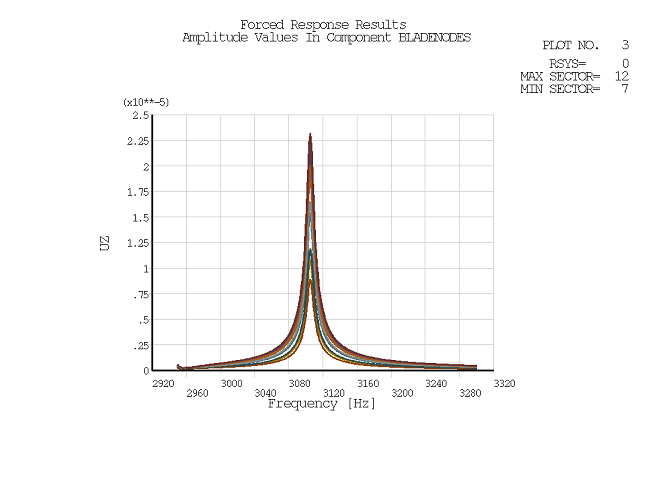
The results may be graphed. PLCFREQ plots the requested specification versus frequency, one curve for each sector as shown in Figure 4.11: CYCSPEC Frequency Response.
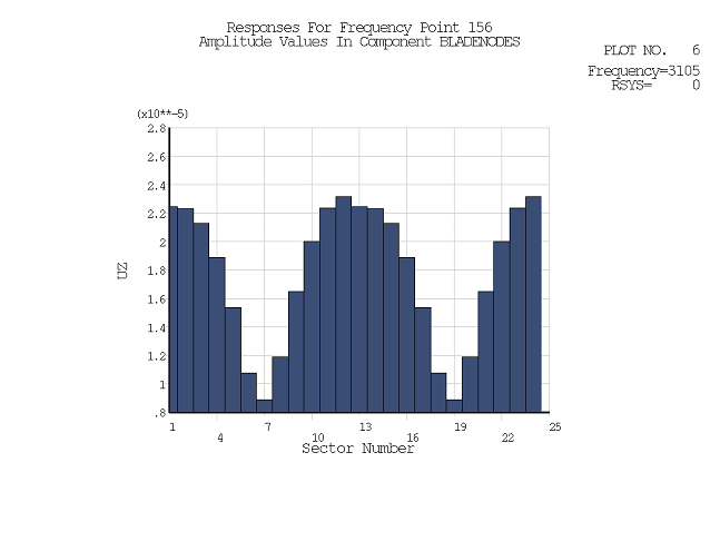
PLCHIST plots a histogram of the requested specification at the requested frequency, one bar for each sector as shown in Figure 4.12: CYCSPEC Histogram Response.
The values in the table may also be retrieved using
*GET or *VGET
(Entity = CYCCALC).
/filname,test

/prep 7
/input,fe_mesh,dat             !Finite element mesh - cyclic symmetry defined
*get,nBlade,common,,cycsym_com,,int,2  ! Determine number of blades: 22 blades
save,baseModel,db,,MODEL
fini

/com,-----------------------------------------------
/com, Pressure Mapping for External Loading
/com,-----------------------------------------------
!* Model already has surface elements
/map
target,pressure_faces
ftype,cfxtbr

!* Read in CFX generated pressures for loading
read,CFXExportLoad_EO2.csv   ! Engine order 2 pressure profile

! CFX and Mechanical blades weren't oriented the same way
! first rotate the blade about the global Z-axis
ngen,2,0,all,,, 0,360*3/nBlade
map,,2,,1,
writemap,CFXLoadEO2.dat
finish

/com,-----------------------------------------------
/com, Pressure Mapping for Aero Coupling
/com,-----------------------------------------------
*DIM,NodalDiamAero,array,22
NodalDiamAero(1)  = 0,1,2,3,4,5,6,7,8
NodalDiamAero(10) = 9,10,11,12,13,14,15,16,17
NodalDiamAero(18) = 18,19,20,21
*get,nAeNDs,PARM,NodalDiamAero,DIM,1

*DIM,AeroFileNames,string,38,22
AeroFileNames(1,1) ='Aero_nodal_dia_zero.csv'
AeroFileNames(1,2) ='Aero_nodal_dia_pos_1.csv'
AeroFileNames(1,3) ='Aero_nodal_dia_pos_2.csv'
AeroFileNames(1,4) ='Aero_nodal_dia_pos_3.csv'
AeroFileNames(1,5) ='Aero_nodal_dia_pos_4.csv'
AeroFileNames(1,6) ='Aero_nodal_dia_pos_5.csv'
AeroFileNames(1,7) ='Aero_nodal_dia_pos_6.csv'
AeroFileNames(1,8) ='Aero_nodal_dia_pos_7.csv'
AeroFileNames(1,9) ='Aero_nodal_dia_pos_8.csv'
AeroFileNames(1,10) ='Aero_nodal_dia_pos_9.csv'
AeroFileNames(1,11) ='Aero_nodal_dia_pos_10.csv'
AeroFileNames(1,12) ='Aero_nodal_dia_pos_11.csv'
AeroFileNames(1,13) ='Aero_nodal_dia_neg_10.csv'
AeroFileNames(1,14) ='Aero_nodal_dia_neg_9.csv'
AeroFileNames(1,15) ='Aero_nodal_dia_neg_8.csv'
AeroFileNames(1,16) ='Aero_nodal_dia_neg_7.csv'
AeroFileNames(1,17) ='Aero_nodal_dia_neg_6.csv'
AeroFileNames(1,18) ='Aero_nodal_dia_neg_5.csv'
AeroFileNames(1,19) ='Aero_nodal_dia_neg_4.csv'
AeroFileNames(1,20) ='Aero_nodal_dia_neg_3.csv'
AeroFileNames(1,21) ='Aero_nodal_dia_neg_2.csv'
AeroFileNames(1,22) ='Aero_nodal_dia_neg_1.csv'

parsav,all,tempMap,parm
parres,change,tempMap,parm
/com,-----------------------------------------------
/com, Mapping for all Aero Coupling IBPA's
/com,-----------------------------------------------
*DO,ii,1,nAeNDs
   /map
   target, Pressure_Faces
   FTYPE, cfxtbr,1
   READ, AeroFileNames(1,ii)
   ! CFX and Mechanical blades weren't oriented the same way
   ! first rotate the blade about the global Z-axis
   ngen,2,0,all,,, 0,360*3/nBlade
   map,,2,,1,
   WRITEMAP, 'mappedIBPA%NodalDiamAero(ii)%.dat'
   finish
*ENDDO

/com,-----------------------------------------------
/com, Blade Alone Mode Shape (NON-CYCLIC) for Aero
/com, Coupling Calculations
/com,-----------------------------------------------
*get,_AeroCoeffJobNm,active,0,jobnam
parsav,all,AeroParm,parm
resume,BeforeMapping,db
parres,new,AeroParm,parm

/prep7
cyclic,off   !Cyclic symmetry is off
fini

/com,-----------------------------------------------
/com, Solution Controls for Static Solve
/com,-----------------------------------------------
/solu
antype,0            ! static analysis
neqit,1,force
pred,off
eqsl,sparse,,,,,1
cntr,print,1        ! print out contact info and also make no initial contact an error
nldiag,cont,iter    ! print out contact info each equilibrium iteration
resc,linear,last    ! Turn on restart files due to future eigen analysis intent
cgom,0,0,1680
nsub,1,1,1
time,1.
stabilize,off   ! Stabilization turned OFF by user
cmsel,s,InterfaceNodes,node ! Select interface nodes between the blade and hub
d,all,all       ! Apply constraints to selected nodes
cmsel,s,BladeElem,elem  ! Select blade elements
nsle
ESEL,A,TYPE,,5  ! also select blade surface elements
solve
fini
/com,-----------------------------------------------
/com, Solution Controls for Perturbed Modal Solve
/com,-----------------------------------------------
/solu
antype,,restart,,,perturbation
perturb,modal,,CURRENT,DZEROKEEP ! pre-stress modal analysis
solve, elform
modopt,lanb,2,0.,3200.
outres,erase
outres,all,none
mxpand,-1,,,no,,no   ! don't expand modes
cgomega,0,0,0
solve
fini

/com,-----------------------------------------------
/com, File Names of Mapped Aero Coupling Pressures
/com,-----------------------------------------------
*DIM,NodalDiamAero,array,22
NodalDiamAero(1)  = 0,1,2,3,4,5,6,7,8
NodalDiamAero(10) = 9,10,11,12,13,14,15,16,17
NodalDiamAero(18) = 18,19,20,21
*get,nAeNDs,PARM,NodalDiamAero,DIM,1

*DIM,AeroMappedFileNames,string,32,nBlade

AeroMappedFileNames(1,1) ='mappedIBPA0.dat'
AeroMappedFileNames(1,2) ='mappedIBPA1.dat'
AeroMappedFileNames(1,3) ='mappedIBPA2.dat'
AeroMappedFileNames(1,4) ='mappedIBPA3.dat'
AeroMappedFileNames(1,5) ='mappedIBPA4.dat'
AeroMappedFileNames(1,6) ='mappedIBPA5.dat'
AeroMappedFileNames(1,7) ='mappedIBPA6.dat'
AeroMappedFileNames(1,8) ='mappedIBPA7.dat'
AeroMappedFileNames(1,9) ='mappedIBPA8.dat'
AeroMappedFileNames(1,10) ='mappedIBPA9.dat'
AeroMappedFileNames(1,11) ='mappedIBPA10.dat'
AeroMappedFileNames(1,12) ='mappedIBPA11.dat'
AeroMappedFileNames(1,13) ='mappedIBPA12.dat'
AeroMappedFileNames(1,14) ='mappedIBPA13.dat'
AeroMappedFileNames(1,15) ='mappedIBPA14.dat'
AeroMappedFileNames(1,16) ='mappedIBPA15.dat'
AeroMappedFileNames(1,17) ='mappedIBPA16.dat'
AeroMappedFileNames(1,18) ='mappedIBPA17.dat'
AeroMappedFileNames(1,19) ='mappedIBPA18.dat'
AeroMappedFileNames(1,20) ='mappedIBPA19.dat'
AeroMappedFileNames(1,21) ='mappedIBPA20.dat'
AeroMappedFileNames(1,22) ='mappedIBPA21.dat'

! Mode normalized by 5.44 when used in CFD
! Mode scaled by 0.5 mm when used in CFD
AeroScaling = (1000/0.5)*5.44

*dim,AeroSpecs,array,3,22
AeroSpecs(1,1)=0,1,1
AeroSpecs(1,2)=1,1,1
AeroSpecs(1,3)=2,1,1
AeroSpecs(1,4)=3,1,1
AeroSpecs(1,5)=4,1,1
AeroSpecs(1,6)=5,1,1
AeroSpecs(1,7)=6,1,1
AeroSpecs(1,8)=7,1,1
AeroSpecs(1,9)=8,1,1
AeroSpecs(1,10)=9,1,1
AeroSpecs(1,11)=10,1,1
AeroSpecs(1,12)=11,1,1
AeroSpecs(1,13)=12,1,1
AeroSpecs(1,14)=13,1,1
AeroSpecs(1,15)=14,1,1
AeroSpecs(1,16)=15,1,1
AeroSpecs(1,17)=16,1,1
AeroSpecs(1,18)=17,1,1
AeroSpecs(1,19)=18,1,1
AeroSpecs(1,20)=19,1,1
AeroSpecs(1,21)=20,1,1
AeroSpecs(1,22)=21,1,1

/prep7
/com,-----------------------------------------------
/com, Compute Aero Coefficients
/com,-----------------------------------------------
aerocoeff,blade,'AeroMappedFileNames','AeroSpecs',AeroScaling,nBlade
/out
*stat,fileAeroArray
/out,scratch

/com,===============================================
/com,===============================================

/com,-----------------------------------------------
/com, Compute Cyclic MSUP Harmonic Solution
/com,-----------------------------------------------
parsav,all,AeroParm,parm
resume,baseModel,db
parres,new,AeroParm,parm

/com,-----------------------------------------------
/com, Cyclic Static LP solve
/com,-----------------------------------------------
/solu
antype,0                   ! static analysis
neqit,1,force              ! Force 1 eq iteration since only nonlinearity is bonded/no sep contact
pred,off
eqsl,sparse,,,,,1
cntr,print,1               ! print out contact info and also make no initial contact an error
nldiag,cont,iter           ! print out contact info each equilibrium iteration
resc,linear,last           ! Turn on restart files due to future eigen analysis intent
cgom,0,0,1680              ! 1680.02/2/PI = 267.38
nsub,1,1,1
time,1.
outres,erase
outres,all,none
outres,nsol,all
outres,rsol,all
outres,strs,all
outres,epel,all
outres,eppl,all
stabilize,off                   ! Stabilization turned OFF by user
/solu
cycopt,msup,1
solve
fini

/com,-----------------------------------------------
/com, Cyclic Modal Solve
/com,-----------------------------------------------
/solu
antype,,restart,,,perturbation
perturb,modal,,CURRENT,DZEROKEEP ! pre-stress modal analysis, only keep zero bcs in case future MSUP
solve, elform                    ! Generate matrices needed for perturbation analysis
modopt,lanb,2,0.,530
outres,erase
outres,all,none
outres,nsol,all
outres,strs,all
outres,epel,all
outres,eppl,all
outres,rsol,all
mxpand,,,,yes,,no       ! expand element results, don't write them to file.mode

cgomega,0,0,0
solve
fini

/post1
file,,rstp
/out,
set,list,,,,,,,order
/out,scratch
/show,png,rev
/yrange,0,530
plzz,16043              ! Plot cyclic modal frequency vs. harmonic index
/show,close
/yrange,default
finish

/com,-----------------------------------------------
/com, Modal Restart for External Loading
/com,-----------------------------------------------
/solu
antype,modal,restart ! restarting the modal analysis
modcont,on
thexpand,off         ! ignore thermal strains
mxpand,,,,yes,,yes   ! expand stress and strain results and write them to file.mode
outres,erase
outres,all,none
outres,nsol,all
outres,strs,all
outres,epel,all
outres,rsol,all
sfedel,all,all,pres
fdele,all,all
cgomega,,0,0,0
/INPUT, CFXLoadEO2,dat !Read in external loading from mapped pressure file
allsel
solve
fini

/com,-----------------------------------------------
/com, Cyclic MSUP Harmonic Solve
/com,-----------------------------------------------
/solu
antype,harm
hropt,msup
thexpand,off     ! ignore thermal strains
hrout,off
harfrq,450.000000,550.000000
kbc,1
nsub,1000

outres,all,all
hrout,on
cycfreq,eo,-2
lvscale,1,1

/com,-----------------------------------------------
/com, Specify Blade Components and Number of Blade
/com, Modes for Mistuning and Aero Coupling
/com,-----------------------------------------------
cycfreq,blade,InterfaceNodes,BladeElem,2

/com,-----------------------------------------------
/com, Specify Mistuning
/com,-----------------------------------------------
*dim,kmist,array,22,1
kmist(1,1) = 0.01,-0.02,0.01,0.04,-0.03,-0.01,-0.02,0.04,0.05
kmist(10,1) = -0.03,-0.02,0.03,-0.04,-0.01,-0.04,0.02,-0.03,0.01,
kmist(19,1) = -0.05,-0.03,0.01,0.01
cycfreq,mist,k,kmist

/com,-----------------------------------------------
/com, Include Aero Coupling Computed Using AEROCOEFF
/com,-----------------------------------------------
cycfreq,aero,fileAeroArray

solve
fini

/post1
/com,-----------------------------------------------
/com, Specify Modal Results (.rst or .rspt) and
/com, Modal Coordinate File (.rfrq)
/com,-----------------------------------------------

cycfiles,file,rstp,file,rfrq
rsys,1

mystep = 77

set,1,mystep
/show,png,rev
/xrange,0,100
plmc,1,mystep,,        ! Plot the modal coordinates from MSUP (Real)
plmc,1,mystep,,1,      ! Plot the modal coordinates from MSUP (Imag)
/show,close

/xrange,default
avprin,,0.3
/cycexpand,,on
/show,png,rev

esel,s,ename,,186
nsle,s,1

/com,-----------------------------------------------
/com, Real Solution
/com,-----------------------------------------------
set,1,mystep,,0
plns,u,z
plns,u,sum
plns,epel,1
plns,s,1
/view,1,0,0,1
plns,u,sum
plns,epel,1
plns,s,1

/com,-----------------------------------------------
/com, Imaginary Solution
/com,-----------------------------------------------
set,1,mystep,,1
plns,u,z
plns,u,sum
plns,epel,1
plns,s,1
/view,1,0,0,1
plns,u,sum
plns,epel,1
plns,s,1

/com,-----------------------------------------------
/com, Compute Amplitudes
/com,-----------------------------------------------
/cycexpand,,phaseang,360
set,1,mystep,
/view,1,1,1,2
plns,u,z
plns,u,sum
/view,1,0,0,1
plns,u,sum
plns,u,z

/com,-----------------------------------------------
/com, Sweep to Get Max Values
/com,-----------------------------------------------
/cycexpand,,phase,sweep
set,1,mystep
/view,1,1,1,2
plns,u,z
plns,u,sum
plns,epel,1
plns,s,1
/view,1,0,0,1
plns,u,sum
plns,epel,1
plns,s,1

/com,-----------------------------------------------
/com, Create Forced Response Data Files and Plots
/com,-----------------------------------------------
mynode = 'TipLE'          !Tip leading edge
cmsel,s,%mynode%
myid = ndnext(0)
alls
set,1,mystep
cycspec,,myid,u,sum
cyccalc,tipTE,csv

plcfreq,1,1,10
plcfreq,1,11,20
plcfreq,1,21,22

/show,close
finish