


A linear perturbation analysis offers simplicity and ease of use. With the aid of a restart from the base analysis, it is easy to envision how the snapshot of the solution matrices from the base analysis is regenerated and used. All other control keys (commands) are optional.
The following topics related to the linear perturbation analysis procedure are available:
- 9.2.1. Process Flow for a Linear Perturbation Analysis
- 9.2.2. The Base (Prior) Analysis
- 9.2.3. First Phase of the Linear Perturbation Analysis
- 9.2.4. Second Phase of the Linear Perturbation Analysis
- 9.2.5. Stress Calculations in a Linear Perturbation Analysis
- 9.2.6. Reviewing Results of a Linear Perturbation Analysis
- 9.2.7. Downstream Analysis Following the Linear Perturbation Analysis
The following figures show the linear perturbation analysis flow for static, modal, eigenvalue buckling, harmonic (full, frequency-sweep VT, or Krylov), and substructure generation pass analyses:


For advanced usage of the above analysis types, controls are available to affect how the snapshot matrices are modified to reflect the real-world engineering applications. These include nonlinear material controls, contact status controls, and loading controls.
The base analysis (the analysis prior to the linear perturbation analysis) can be a linear or nonlinear, static or full (TRNOPT,FULL) transient analysis. The nonlinearity in the base analysis can be due to nonlinear materials, geometric nonlinearity, or nonlinear contact elements being used.
If the base analysis includes contact elements, it is highly recommended that you turn on the large deflection option (NLGEOM,ON). Otherwise, the algorithms that bond the contact interface use the original, undeformed geometry for NLGEOM,OFF, which might lead to an inaccurate solution (or possibly a memory error in the case of linear perturbation eigenvalue buckling) if there is significant deformation in the base analysis.
If the base analysis is linear static only (that is, only prestress effects are to be included in the model), the multiframe restart option must be invoked by using the RESCONTROL,LINEAR command, which is a non-default option for linear static analysis.
If the base analysis is a nonlinear static analysis or a nonlinear or linear full transient analysis, the multiframe restart is automatically invoked. However, you can use the RESCONTROL command to tell the program at which time points the necessary data is to be saved for the multiframe restart. Only the converged substeps of the load step are saved for a multiframe restart, thereby automatically guaranteeing that a valid restarting point is used for the linear perturbation analysis.
The following files must be saved from the base analysis for use in the restart performed as the first phase of the linear perturbation procedure:
| Jobname.rdb - Mechanical APDL database file |
| Jobname.ldhi - Load history file |
Jobname.Rnnn
- Element saved records (restart files) |
You can include inertia relief to simulate a minimally restrained structure in a linear perturbation static analysis or a linear perturbation eigenvalue buckling analysis provided that the base analysis is static. To include inertia relief, issue IRLF,1 before the SOLVE command in the static base analysis (for details, see Inertia Relief in a Linear Perturbation Static Analysis in the Basic Analysis Guide).
For more information on these files and the multiframe restart procedure, see Restarting an Analysis in the Basic Analysis Guide
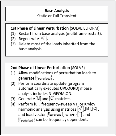
The purpose for the first phase in the linear perturbation analysis procedure is to regenerate the solution snapshot from the base analysis. Normally, this phase only requires the following command input:
/SOLU
ANTYPE,,RESTART,loadstep,substep,PERTURB
....  ! (other limited commands are allowed)
PERTURB,MODAL    ! can be STATIC, MODAL, BUCKLE, HARMONIC (full, VT, or Krylov harmonic), or SUBSTR
SOLVE,ELFORM
! (do not exit solution module yet; do not issue FINISH command)
Upon execution of the SOLVE,ELFORM command, the program
restarts the base analysis and regenerates
 material data needed for the subsequent perturbation analysis and
other possible solution matrices. Then, by default, the program removes all external
loads inherited from the base analysis, except for displacement boundary conditions,
inertia loads, and all non-mechanical loads (including thermal loads).
material data needed for the subsequent perturbation analysis and
other possible solution matrices. Then, by default, the program removes all external
loads inherited from the base analysis, except for displacement boundary conditions,
inertia loads, and all non-mechanical loads (including thermal loads).
Since this phase is strictly used to regenerate solution matrices from the base analysis, no other actions (commands) are needed in most cases. The following items can be modified, however, so that the final solution matrices used in the linear perturbation analysis can serve various purposes for the engineering analysis:
To perform a partial nonlinear prestressed modal analysis for brake squeal simulation, issue the CMROTATE command.
Modify element real constants (RMODIF). For example, if contact stiffness in the base analysis is low (which is usually the case when small loads are applied in the base analysis), use RMODIF to increase the contact stiffness so that the interface is more strongly bonded for the downstream analysis.
Modify material properties (TBMODIF or MP command); for example, to change the contact friction coefficient.
Material behavior can be controlled via the PERTURB command. (For more information, see Material Properties of Structural Elements in Linear Perturbation in the Element Reference.)
To include Coriolis effects in the modal analysis when the base analysis is static, issue the CORIOLIS command.
To allow the domain decomposition method for linear perturbation harmonic analyses, issue the DDOPTION command.
If inertia relief was included in the base analysis of a linear perturbation static analysis or a linear perturbation buckling analysis, the inertia relief load is recalculated to include the prestressed matrix by default.
To exclude this inertia relief load vector and its effects you must issue IRLF,0 in the first phase of the linear perturbation static analysis.
For a linear perturbation eigenvalue buckling analysis, you may exclude the inertia relief load vector if the base analysis is nonlinear by issuing IRLF,0 in the first phase of the perturbed buckling analysis. If the base analysis is linear, the inertia load should be included in the perturbation phase.
For details, see Inertia Relief in a Linear Perturbation Static Analysis in the Basic Analysis Guide and Linear Perturbation Static Analysis with Inertia Relief.
Other commands that are allowed in this phase of the linear perturbation analysis are: EALIVE, EKILL, and ESTIF.
It is important to understand which matrices are used in the linear perturbation analysis:
If the base analysis is nonlinear, the consistent tangent matrix from the prior Newton-Raphson iterations is regenerated based on the material behavior specified by the PERTURB command and based on the current geometry configuration if large-deflection effects are included (NLGEOM,ON).
If contact elements are present in the base analysis, the stiffness matrix includes the effects of contact based on the contact status (set via PERTURB or CNKMOD).
If the base analysis is linear, the linear stiffness matrix plus the stress stiffening matrix is used (automatically included).
The spin-softening or gyroscopic effect is also included in this matrix regeneration phase as long as this spin-softening or gyroscopic effect is included in the base analysis.
Other commands such as PSTRES, EMATWRITE, OMEGA, and CMOMEGA are not needed in this phase, as they are accounted for automatically.
The second phase of a linear perturbation analysis is performed immediately following the SOLVE,ELFORM command from the first phase without exiting the solution processor (/SOLU); this is in order to correctly retain the snapshot of the restart status from the base analysis. Also, for the case of geometric nonlinearity, the nodal coordinates are updated automatically based on the restart point (you do not need to issue the UPCOORD command).
The second phase of the linear perturbation analysis varies slightly depending on whether you are performing a static, modal, eigenvalue buckling, or harmonic (full, frequency-sweep (VT), or Krylov) analysis. Details for each type of linear perturbation are discussed in the following sections.
As described in Figure 9.1: Flowchart of Linear Perturbation Static Analysis, the second phase of a linear perturbation static analysis consists of the following actions:
Apply linear perturbation loads to generate {Fperturbed}. (Note that thermal loads can be applied in the second phase of a linear perturbation static analysis. See Generating and Controlling Non-mechanical Loads for more information.)
If the base analysis included large deflection (NLGEOM,ON), update the nodal coordinates by using the total displacement from the base analysis (similar to the UPCOORD command, but executed automatically and internally in this phase). From this point on, the deformed mesh is used for calculating perturbation loads and for postprocessing results from the linear perturbation analysis.
Perform the linear perturbation static analysis to solve
 .
.
User action is needed only for the steps 1 and 3 shown above. The program performs step 2 automatically. (See Static Analysis Based on Linear Perturbation in the Theory Reference.)
The following example shows typical command input to accomplish these steps.
Example Input for Linear Perturbation Static Analysis
F,NODE,...   ! Add linear perturbation loads
...
TIME,... 		! End time
SOLVE
FINISH
In a linear perturbation static analysis, the strain/stress calculation is done within the time substeps as it is in a standard static analysis.
Although a linear perturbation static analysis is a linear static analysis, these differences from a linear static analysis should be noted:
The linear perturbation static analysis treats the process as a one-step analysis. It internally enforces the command NSUBST,1,1,1 and ignores user-specified inputs entered via the NSUBST or DELTIM commands.
If the base analysis is nonlinear and the tangent matrix becomes nearly singular (for example, reaching the nonlinear buckling point) or indefinite (for example, a plastic hinge) at the restart point, then a message concerning negative or small pivots may be printed out from the linear perturbation static analysis. This typically does not happen in a purely linear static analysis if the model is properly constrained. When this occurs in a linear perturbation analysis, it is your responsibility to verify the correctness of the solution.
If the base analysis is purely linear, then the linear perturbation static analysis could result in total stiffness matrices having large negative pivots or small pivots, depending on the prestressed effect (stress stiffening) introduced by the linear base analysis.
For an example using linear perturbation for a static analysis see Example 9.1: Linear Perturbation Static Analysis.
As described in Figure 9.2: Flowchart of Linear Perturbation Modal Analysis, the second phase of a linear perturbation modal analysis consists of the following actions:
Apply linear perturbation loads to generate {Fperturbed}. (Note that thermal loads can not be applied in the second phase of a linear perturbation modal analysis. See Generating and Controlling Non-mechanical Loads for more information.)
If the base analysis included large deflection (NLGEOM,ON), update the nodal coordinates by using the total displacement from the base analysis (similar to the UPCOORD command, but executed automatically and internally in this phase). From this point on, the deformed mesh is used for calculating perturbation loads and for postprocessing results from the linear perturbation analysis.
Regenerate other needed matrices such as mass and damping matrices ([M] and [C]).
Perform the linear perturbation modal analysis.
User action is needed only for steps (1) and (4) shown above. The program performs steps (2) and (3) automatically (see Modal Analysis Based on Linear Perturbation in the Mechanical APDL Theory Reference).
The following example shows typical command input to accomplish these steps.
Example Input for Linear Perturbation Modal Analysis
MODOPT,eigensolver,number_of_modes,
. . .       (include commands to add or remove linear perturbation loads)
MXPAND,number_of_modes,
SOLVE
FINISH
In a linear perturbation modal analysis, after the solution phase, a stress expansion pass is typically carried out. A stress expansion must be done along with the modal analysis in order to use the appropriate material property and to obtain the total sum of elastic strain/stress due to the linear perturbation analysis and the base analysis. A separate expansion pass (EXPASS command) is not allowed after the linear perturbation analysis.
For examples using linear perturbation modal analysis see:
As described in Figure 9.3: Flowchart of Linear Perturbation Eigenvalue Buckling Analysis, the second phase of a linear perturbation eigenvalue buckling analysis consists of the following actions:
Apply linear perturbation loads to generate {Fperturbed}. (Note that thermal loads can be applied in the second phase of a linear perturbation eigenvalue buckling analysis. See Generating and Controlling Non-mechanical Loads for more information.)
Solve for {Uperturbed} from
 . This step is executed automatically and
internally by the program.
. This step is executed automatically and
internally by the program.Generate the linear stress stiffness matrix
 using {Uperturbed}. This
step is executed automatically and internally by the program.
using {Uperturbed}. This
step is executed automatically and internally by the program.If the base analysis included large deflection (NLGEOM,ON), update the nodal coordinates by using the total displacement from the base analysis (similar to the UPCOORD command, but executed automatically and internally in this phase). From this point on, the deformed mesh is used for calculating perturbation loads and for postprocessing results from the linear perturbation analysis.
Perform the linear perturbation eigenvalue buckling analysis to solve
 , where ϕj are the
eigenvectors and λj are the
eigenvalues.
, where ϕj are the
eigenvectors and λj are the
eigenvalues.
In a linear perturbation eigenvalue buckling analysis, the perturbation load {Fperturbed} does not include external loads introduced by contact gaps or penetrations, even if these loads were applied in the prior static or transient load steps.
Note: The procedure that the Mechanical APDL solver uses to evaluate buckling load factors depends on whether the prestressed base analysis is linear or nonlinear.
For a linear base analysis:
You can define loading only in the base static structural analysis prior to the eigenvalue buckling analysis.
The eigenvalues calculated by the buckling analysis represent buckling load factors that scale all of the loads applied in the static structural analysis.
The buckling load is calculated by the perturbation load multiplied by the eigenvalues,
 .
. For more details and considerations on setting up the static structural base analysis prior to the buckling analysis, see Step 2. Obtain the Static Solution.
For a nonlinear base analysis:
In the buckling analysis phase, you must define additional loading which is different from the total loads at the restart point,
 , in the upstream static structural base
analysis.
, in the upstream static structural base
analysis.You must manually calculate the buckling load as the sum of the total loads in the static structural analysis at the specified restart load step plus the perturbation loads applied in the buckling analysis multiplied by the eigenvalue or buckling load factor for the jth mode:
 .
.
User action is needed only for steps (1) and (5) shown above. The program performs steps (2), (3), and (4) automatically. For a more detailed description of the theory and governing equations for linear perturbation eigenvalue buckling analysis see Eigenvalue Buckling Analysis Based on Linear Perturbation in the Theory Reference.
The following example shows typical command input to accomplish these steps.
Example Input for Linear Perturbation Buckling Analysis
BUCOPT,eigensolver,number_of_modes,
. . .       (include commands to add or remove linear perturbation loads)
MXPAND,number_of_modes,
SOLVE
FINISH
Generally, the Block Lanczos eigensolver (BUCOPT,LANB) performs well for perturbed eigenvalue buckling analyses. However, when the tangent stiffness matrix becomes indefinite, the Block Lanczos eigensolver could fail to produce an eigensolution due to the mathematical limitation of this solver (refer to Eigenvalue Buckling Analysis Based on Linear Perturbation for more information on when this could occur.) In this case, it is recommended that you use the subspace eigensolver (BUCOPT,SUBSP) to achieve a successful solution.
In a linear perturbation buckling analysis, after the solution phase, a stress expansion pass is typically carried out. A stress expansion must be done along with the buckling analysis in order to use the appropriate material property and to obtain the total sum of elastic strain/stress due to the linear perturbation analysis and the base analysis. A separate expansion pass (EXPASS command) is not allowed after the linear perturbation analysis.
For an example using linear perturbation buckling analysis, including a linear (case 1) and nonlinear (case 2) base analysis, see Example 9.6: Using Linear Perturbation to Predict a Buckling Load.
As described in Figure 9.4: Flowchart of Linear Perturbation Harmonic Analysis, the second phase of a linear perturbation harmonic analysis (full, frequency-sweep VT, or Krylov method) consists of the following actions:
Apply linear perturbation loads to generate {Fperturbed}. (Note that thermal loads cannot be applied in the second phase of a linear perturbation harmonic analysis. See Generating and Controlling Non-mechanical Loads for more information.)
If the base analysis included large deflection (NLGEOM,ON), update the nodal coordinates by using the total displacement from the base analysis (similar to the UPCOORD command, but executed automatically and internally in this phase). From this point on, the deformed mesh is used for calculating perturbation loads and for postprocessing results from the linear perturbation analysis.
Regenerate the needed matrices such as mass and damping matrices ([M] and [C]).
Perform the linear perturbation harmonic analysis.
User action is needed only for steps (1) and (4) shown above. The program performs steps (2) and (3) automatically (see Harmonic Analysis Based on Linear Perturbation in the Mechanical APDL Theory Reference for more information.)
The following example shows typical command input to accomplish these steps.
Example Input for Linear Perturbation Harmonic Analysis
HROPT,FULL
. . .       (include commands to add or remove lilnear perturbation loads)
HARFRQ,beginning_frequency,end_frequency
NSUB,number_of-frequency_steps
SOLVE
FINISH
In a linear perturbation harmonic analysis, the strain/stress calculation is done within the frequency substeps as it is in a standard full or frequency-sweep harmonic analysis.
For an example using linear perturbation harmonic analysis see Example 9.7: Linear Perturbation (Prestressed) Harmonic Analysis.
In this section, the term substructure refers to substructuring and CMS analyses. As described in Figure 9.5: Flowchart of Linear Perturbation Substructure Generation Pass, the second phase of a linear perturbation substructure generation pass consists of the following actions:
Apply linear perturbation loads to generate {Fperturbed}. The perturbation load is the first load vector in the substructure generation.
If the base analysis included large deflection (NLGEOM,ON), update the nodal coordinates by using the total displacement from the base analysis (similar to the UPCOORD command, but executed automatically and internally in this phase). From this point on, the deformed mesh is used for calculating perturbation loads and for postprocessing results from the linear perturbation analysis.
Add specifications for the substructure file name, master degrees of freedom, method (for example, CMS method), and matrices to generate.
Perform the linear perturbation substructure generation pass to generate reduced matrices requested via the command SEOPT,,
SEMATR(stiffness matrix only; or stiffness and mass matrices; or stiffness, mass, and damping matrices) and to generate the reduced perturbation load.
User action is needed only for steps (1), (3), and (4) shown above. The program performs step (2) automatically (see Substructure or CMS Generation Based on Linear Perturbation in the Mechanical APDL Theory Reference.)
The following example shows typical command input to accomplish steps (3) and (4).
Example Input for Linear Perturbation Substructure Generation
M,NODE,ALL,...   ! Specify Master Degrees of Freedom on Nodes
...
SEOPT,SuperE,3   ! Generate stiffness, mass, and damping matrices
CMSOPT,FIX...    ! Specify CMS method
SOLVE
FINISH
The more straightforward procedure is to use the linear perturbation substructure generation pass to treat the entire model from the base analysis as one substructure (see Example 9.8: Linear Perturbation Substructure Generation Pass Followed by Use and Expansion Passes).
Nevertheless, selecting portions of the model from the base analysis to do multiple substructure generation passes is supported, but this requires you to manage files in the following steps of the analysis:
You must copy files at the end of each generation pass in order to perform the expansion passes.
For a discussion on the required files see Step 3: Expansion Pass in the Substructuring Analysis Guide for substructuring and The CMS Use and Expansion Passes in the Substructuring Analysis Guide for CMS.
Use the /COPY command for each requested file or issue SEOPT with
LPnameKey= ON.
Because the expansion passes are done from the database of the entire model, non-superelement portions exist in the results file, and the CMSFILE command cannot be used to visualize the entire expanded assembly on these result files.
In such cases, the expanded results of each superelement must be selected and rewritten in intermediate .RST files to be correctly combined with the CMSFILE command (with
CmsKey= OFF). For more information, see Example 9.9: Linear Perturbation Substructure with Two Generation Passes, Use Pass, and Two Expansion Passes.
If the base analysis is nonlinear and the tangent matrix becomes nearly singular (for example, reaching the nonlinear buckling point) or indefinite (for example, a plastic hinge) at the restart point, then a message concerning negative or small pivots may be printed out from the linear perturbation substructure generation pass. This typically does not happen in a purely linear substructure generation pass if the model is properly constrained. When an indefinite matrix occurs in a linear perturbation substructure generation pass, it is your responsibility to verify the correctness of the solution.
The following are assumptions related to the use and expansion passes following a linear perturbation substructure generation pass:
The generated substructure is assumed to be linear and can be used in a subsequent use pass. The use pass does not require a linear perturbation procedure.
In the expansion pass, all material properties are assumed to be linear, and all contact statuses are frozen as in a linear application. NLGEOM is turned OFF, even if the base analysis for the prestressed substructure generation pass is nonlinear. The expansion pass does not require a linear perturbation procedure.
For examples using linear perturbation substructure generation pass see:
Just as in a standard linear analysis, once the solution eigenvectors or harmonic solution are available, the stresses or strains of the structure can be calculated.
In general, two choices are available for calculating incremental (perturbation) stresses, depending on PERTURB command settings and base material properties. By default, the program uses the linear portion of the nonlinear material constitutive law to recover stresses for all materials, except for hyperelasticity. For hyperelasticity, the material property is based on the tangent of the hyperelastic material's constitutive law at the restart point.
Because a linear perturbation analysis can be understood as an extra iteration of the base analysis, all history-dependent results of the base analysis are inherited in the results of the linear perturbation analysis. Therefore, any plastic strains, creep strains, swelling strains, and contact results from the base analysis are available in the results data of the linear perturbation analysis.
The total strain is the sum of all strains (for example, PLNSOL,EPTO). The nonlinear solution quantities such as equivalent stress, stress state ratio, and plastic state variable are also available. For detailed information about element results from a linear perturbation analysis, see Interpretation of Structural Element Results After a Linear Perturbation Analysis in the Element Reference.
For contact elements, the contact status or contact forces are frequently of interest. The program uses the same contact status in calculations of both the stiffness matrix for the linear perturbation analysis and contact results for the expansion pass.
In the linear perturbation analysis, the program calculates all requested results, including stresses and strains, and stores them in the Jobname.rstp file. One reason for the creation of the Jobname.rstp file is that all the existing restart files from the base analysis are preserved for possible future use. The same linear perturbation or restart analysis can be performed repeatedly from the same restarting point. The Jobname.rstp file only stores the results of the linear perturbation analysis. Results of the base analysis are still stored in the Jobname.rst file.
The stresses at the restarting point of the base static or full transient analysis should be obtained from the Jobname.rst file of the base analysis.
Note: When postprocessing results obtained in a separate session, you must resume the database saved after the linear perturbation analysis solution is finished, because the node coordinates have been updated with the base analysis displacements during the solve.
Note: When postprocessing the base analysis results, you must resume the database that was saved before the linear perturbation analysis.
Following the linear perturbation analysis, other analysis types can be performed by using the information from the linear perturbation analysis.
If the linear perturbation analysis is a modal analysis, the following analysis types are possible by using the Jobname.mode file generated by the perturbation and the database of the model:
Harmonic or transient analysis using the mode-superposition method (HROPT,MSUP or TRNOPT,MSUP). Mode-superposition analysis based on QRDAMP eigensolver is not supported.
The eigenmode reuse procedure (Restarting a Modal Analysis) is also available for linear perturbation analysis.
Response spectrum analysis
Random vibration analysis
The deformed mesh due to the prior static or full transient analysis is used in the linear perturbation analysis and in the downstream analysis. As such, the database used for the downstream analysis should correspond to the deformed mesh (after the linear perturbation solve).
In all analyses listed above, the first load vector used is {Fperturbed}. If more loading cases are required, a new {Fperturbed} load vector must be generated ( MODCONT). The program assumes purely linear analyses and uses linear material properties, even for all nonlinear materials.